Catching ghosts with a coarse net: use and abuse of spatial sampling data in detecting synchronization

Abstract

Synchronization of population dynamics in different habitats is a frequently observed phenomenon. A common mathematical tool to reveal synchronization is the (cross)correlation coefficient between time courses of values of the population size of a given species where the population size is evaluated from spatial sampling data. The corresponding sampling net or grid is often coarse, i.e. it does not resolve all details of the spatial configuration, and the evaluation error—i.e. the difference between the true value of the population size and its estimated value—can be considerable. We show that this estimation error can make the value of the correlation coefficient very inaccurate or even irrelevant. We consider several population models to show that the value of the correlation coefficient calculated on a coarse sampling grid rarely exceeds 0.5, even if the true value is close to 1, so that the synchronization is effectively lost. We also observe ‘ghost synchronization’ when the correlation coefficient calculated on a coarse sampling grid is close to 1 but in reality the dynamics are not correlated. Finally, we suggest a simple test to check the sampling grid coarseness and hence to distinguish between the true and artifactual values of the correlation coefficient.

1. Introduction

Evaluation of properties of a spatially extended system from sparse spatial data is an inherent problem in many applications across science and engineering [1–3]. The term ‘sparse data’ usually refers to a situation where the information about a spatial distribution of a certain quantity (e.g. the concentration of a chemical substance in the environment) is available only at nodes of a certain discrete grid or net, and the number of grid nodes is not large enough to resolve the details of the heterogeneous distribution of the substance and/or the spatial configuration of the system. Often sparse spatial data are used to evaluate an integral property of the system—say, a ‘total mass’, the exact meaning of which depends on particular application. Here, we mention just a few examples: in water quality engineering, it is the total amount of a harmful chemical substance occasionally released into the environment [1]; in geology, it is the total stock of a valuable mineral [2,4]; in medicine, it is the total mass of a tumour [5]; and in ecology, it is the population size of a dangerous pest [3,6,7]. A generic problem for the above examples, as well as for other similar situations where researchers or engineers have to deal with sparse data, is that, due to the apparent loss of information, the evaluation of the total mass can produce a result of unacceptably low accuracy. In its turn, that can lead to wrong decisions and dramatic consequences, e.g. a large reserve of a valuable mineral is overlooked, a dangerous tumour is not treated timely, etc.

In this paper, we consider the problem of sparse data in the context of ecological applications. Information about population abundance is routinely used in ecology for many different purposes such as to assess the ecosystem state and biodiversity [8,9], to identify and monitor endangered species [10,11], to monitor pests [12], to account for some important properties of population dynamics (e.g. spatial patterning [13,14] or synchronization [15–19]), etc. While theoretical studies usually assume that this information—e.g. as quantified by the population size or the population density—is readily available with any required precision, estimation of population abundance in empirical studies is rarely straightforward. For instance, evaluation of the population size by direct counting is only possible for some species and only in relatively small habitats. Much more often, collection of relevant field data involves a certain sampling procedure [3]. Samples are taken across space with the intention to provide an estimate of the population density of a given species at some particular locations inside a given area or habitat [7,20] (figure 1). The accuracy of the population abundance evaluation depends on the accuracy of the local population density estimate at the location of a given sample and on the sample size (i.e. the total number of samples in a given census). It can also depend on the way in which the local data are pulled together or ‘integrated’ to produce an estimate of the population size [21,22].

Figure 1.

(a) A sketch of sampling on a coarse grid along a one-dimensional transect. The dashed curve shows a hypothetical population distribution which is only known at the location of samples. (b) Population density u(x,y) of a carabid beetle species in a farm field obtained from data collected on a fine grid of 16 × 16 traps (data from [13]). The large black dots show the location of the nodes of a hypothetical coarse sampling grid of 3 × 3 nodes. Apparently, in both cases shown in panels (a,b), the sampling data obtained on a coarse grid would miss some important details of the population distributions. (Online version in colour.)

We mention here that the accuracy of the local data depends on the nature of the samples which, in its turn, depends on the species traits. For instance, for soil-dwelling insects, sampling is often done by taking soil cores [7,12,23]. The insect count in a given soil core gives an almost perfect estimate of the local population density. For flying insects or insects walking/crawling on the surface, their census is usually done by installing traps and subsequently analysing trap counts, a procedure that inevitably introduces a certain error [6,24]. The precision of the local population density estimation and the number of samples collected in a population census, albeit not being entirely independent,¹ are affected by largely different factors. As in this paper our main goal is to understand how the reliability of conclusions about population dynamics (in particular, synchronization) can be affected by the samples size, we assume that local data are precise. The only source of the evaluation error is then the coarseness of the sampling grid.

In sampling procedures, both the location of the samples and their total number (to which altogether we refer as a sampling grid) used in any one given census or population survey are chosen based on a variety of reasons. A closer look at the corresponding arguments reveals that, while in some cases they are theory-based (e.g. based on the analysis of variances [25,26]) in many other cases the properties of the sampling grid are decided based on a rule of thumb [27]. The question hence arises as to when—i.e. under what conditions—the population size estimated from data collected over a given sampling grid is accurate enough to provide a reliable information for any conclusions about the system properties and/or dynamics. In our previous work [6,21,22,28], we showed that the above question ‘when’ has a relative rather than absolute meaning as the evaluation accuracy depends on the spatial pattern of the population distribution. The same sampling grid may provide a very accurate estimate of the population size for one spatial population distribution but can lead to a completely wrong result for another distribution.

The main goal of this study is to consider how the quality of sampling data affects the conclusions on the presence or the absence of synchronization between population fluctuations in different habitats. Synchronization is frequently reported in the literature [15–19,29–37]; however, technical details of the data collection, such as the properties of the sampling grid, are often omitted. Also, the effect of the spatial pattern in the distribution of the corresponding populations usually remains obscure. Therefore, at least in some cases, the question may arise as to whether the observed synchronization is really as strong as it is reported. We will focus on the rather common case where the sampling grid is coarse, i.e. where the total number of samples taken in a given area is not large. We will show that sampling over a coarse sampling grid can lead to wrong conclusions, because synchronization remains undetected. We will also show that sampling over a coarse grid can result in a ‘ghost synchronization’ where synchronization is seen in the data while in reality the monitored populations are not synchronized.

2. Mathematical framework

Consider a generic case where a certain population described by its population density is sampled in a given domain A. The domain may be the species habitat or it may be defined by some external factors or tasks.² Although the results of our analysis are going to be rather general and not restricted to any particular species or taxa, for the convenience of interpretation we will mostly talk about invertebrates, e.g. insects, worms or slugs. In the case of an invertebrate population, its sampling is usually done by installing traps and then analysing the trap counts [6,38,39] or by taking soil cores and counting the number of individuals in each core [7,12]. For simplicity, we assume that all samples in the given census are taken over a sufficiently small period of time, so that the population density would not undergo any significant change during the census duration. In mathematical terms, this standard sampling procedure provides the information about the population density as a set of values where is the location of the ith sample, N is the number of samples in the given census and t is the timing of the census. This information is then processed to produce a certain index that quantifies the population abundance in the given area. Quite often, the sampling data are used to obtain an estimate of the population size ω_A or the average population density where Z_A is the area of the domain. There are several ways to calculate the average density [22]; in this study, we consider the method commonly used in empirical ecology [3,7] to estimate the average by calculating the arithmetic mean of the sampled values:

2.1

In the case where the census is done regularly, say at times t₁, t₂,…, t_k, application of (2.1) to the samples collected in each census results in a time series of the average population densities, i.e. . This time series can then be further analysed depending on the purpose of the study. When the study focuses on synchronization, sampling procedure is applied to a number of domains/habitats to produce the corresponding number of different time series. For example, sampling in domains A and B would produce two time series, and , respectively. The standard statistical tool to reveal synchronization is the (cross)correlation coefficient [18,29,30,31]:

2.2

where and μ_B are the sample means of the time series S_A and S_B:

2.3

It follows from (2.2) that −1 ≤ ρ ≤ 1 where 0 < ρ ≤ 1 corresponds to correlation and −1 ≤ ρ < 0 to anti-correlation.

Depending on the calculated value of ρ, i.e. on the correlation strength, a conclusion can be made about the existence or the absence of synchronization if ρ is close to one or close to zero, respectively. We mention here that the notion of ‘correlation strength’ used in ecological studies is somewhat conventional [40]: the correlation is regarded as very strong for 0.8 ≤ ρ ≤ 1, strong for 0.6 ≤ ρ < 0.8, moderate for 0.4 ≤ ρ < 0.6, weak for 0.2 ≤ ρ < 0.4 and very weak for 0 ≤ ρ < 0.2. We will use this verbal description of the correlation strength in our analysis below. Apparently, there is considerable difference in the population dynamics, and hence different implications, depending on whether the population fluctuations in different domains over a given area are synchronized (strongly correlated) or not synchronized (very weakly correlated). For instance, the existence of synchronization may result in population outbreaks or population falling to low numbers not in a single habitat but over vast areas of space, and hence may pose considerable problems for pest control or nature conservation [12,18,29,41].

We emphasize that, although the right-hand side of equation (2.2) does not contain the number of samples N explicitly, the correlation coefficient does depend on N because the values of average population density and depend on N. It is an inherent problem with expression (2.1) (as well as, in fact, with any other way to calculate ) that its accuracy depends on N. A small number of samples can make the accuracy very low. Importantly, the number of samples required for a sufficiently accurate estimate is known to strongly depend on the properties of the population distribution [6,21,22]. For an approximately uniformly distributed population, a few samples can provide a very good estimate of the average density (ultimately, just one sample is enough if the distribution is exactly uniform). However, for a strongly heterogeneous or even ‘patchy’ distribution where the density exhibits large-amplitude fluctuations over space, a reasonable accuracy can only be achieved with a much larger number of nodes in the sampling grid, i.e. when all the peaks in the population distribution are somehow ‘resolved’ [21,42]. On a coarse grid, i.e. where the number of nodes is not sufficiently large to resolve the details of patchy distribution, the evaluation accuracy can become poor. In particular, in the examples shown in figure 1, it is readily seen that the arithmetic average of the locally sampled population density would significantly underestimate the true value as the population peaks remain unresolved. The large numerical error of evaluating the average density on a coarse grid, i.e. the difference between the right-hand side in (2.1) and the true value , is then carried on to the corresponding time series and therefore can significantly affect the calculated value of the correlation coefficient and hence the conclusions about the presence or the absence of synchronization. In §§3 and 4, this heuristic inference will be confirmed by a detailed quantitative analysis of several case studies.

3. Synchronization ‘lost and found’: instructive example

Since synchronization in a system of multiple domains is usually considered pairwise, cf. equation (2.2), it is sufficient for our purposes to consider a system consisting of just two domains, A and B. In this section, we restrict our analysis to the one-dimensional case so that the domains are quantified by their lengths (rather than area) which we assume to be the same, L_A = L_B = L.

The idea of our analysis is to consider a system with some known, prescribed properties and to show how these properties may become obscure or distorted when the sampling grid is coarse. Specifically, we simulate two sequences of spatial population distributions, different in A and B, the corresponding total population sizes (or the average population densities) being certain known functions of time. These functions, ω_A(t) and ω_B(t), respectively, describe the ‘population dynamics’, i.e. how the population sizes in domains A and B are evolving with time. For the purposes of this section, we consider a strong test where these functions are identical, . Thus, the population dynamics in A and B is perfectly synchronized and the theoretical value of the correlation coefficient (2.2) is exactly one. The question that we are going to consider is what can be the empirical value of the correlation coefficient for different value N of nodes in the spatial sampling grid.

The ways to generate ‘realistic’ heterogeneous population densities u_A(x,t) and u_B(x,t) are numerous; for instance, they can be obtained from a population dynamics model [43]. Here, we use a simpler approach: we consider the population density being a superposition of normal distributions:

3.1

where t=1,2,…,k are the moments when the census is taken (e.g. weekly, monthly or annually),

3.2

where parameter σ is the standard deviation, and the peak locations are independent identically distributed random variables drawn from a certain probability distribution for every peak and every year. Parameter p has the meaning of the number of peaks in the distribution, although some of the peaks can merge or nearly merge when their location is close. The single-peak distribution (p = 1) can be regarded as a case of high population aggregation while the multi-peak case corresponds to a case where the population is somehow distributed over the whole domain. Examples of function (3.1) are shown in figure 2.

Figure 2.

An example of the superposition u(x) of normal distributions for p = 4 (a) and p = 8 (b) as given by equations (3.1) and (3.2) with ω(t) = C(t + 1) for C = 20 and t = 375.

Integration of the population density (3.1) gives the population size. In the unbounded domain , the Gaussian distribution (3.2) is scaled to one, so that

3.3

therefore ω is indeed the population size. In the case where the population (3.1) is considered in the bounded domain 0<x<L,

3.4

because the tail of the distribution lies outside of the domain. Moreover, considering the location of each peak to be a random variable uniformly distributed over the domain, the deviation |M−ω| can be considerable (in the single-peak case it can be as large as ω/2, i.e. 50% of the total). To reduce the effect of this random fluctuation in the population size, we consider the model where the location of each peak is drawn from a uniform probability distribution defined over a truncated domain ε < x<L−ε where the auxiliary parameter ε is chosen sufficiently large compared with the standard deviation σ to provide .

With regard to the population dynamics, we begin with the simple hypothetical case where the population size grows linearly with time, i.e. ω(t)=C(t + 1) where C is a certain constant parameter. For this system, we consider the series of k = 500 censuses and, correspondingly, generate 500 population distributions for each domain A and B.

We then consider the sequence of sampling grids with the number of nodes N increasing from N = 1 to N = N_max. For every given N, the sampling grid is centred around the domain midpoint and the grid nodes (i.e. the location of the sampling points across space) are distributed uniformly over the domain with constant spacing Δx between the neighbouring nodes:

3.5

where Δx=L/(N+1). For every given N, each of the generated population distributions is sampled on the corresponding grid and the average population density (2.1) is calculated. The time course of values of the average population density obtained for a given N is then fed into equations (2.2) and (2.3) to calculate the corresponding value of the correlation coefficient. Correspondingly, the correlation coefficient becomes a function of the number of grid nodes, ρ = ρ(N), where for the sake of simplicity we now omit A, B and k from the notation for the correlation coefficient but emphasize its dependence on N.

Figure 3 shows the results obtained for a highly aggregated single-peak population distribution, i.e. equation (3.2) with p = 1 and σ = 8.0. The domain length is L = 300, truncation is done with ε = 40. We observe that the truncation of the domain at the ends to generate the distribution (3.1) is indeed necessary to correctly describe the highly correlated dynamics between the two domains, with ρ ≈ 1. In the case where the domain is not truncated, ρ does not approach one even for a very large N. In the rest of this section, we therefore stick to the case where the location of each peak is a random variable uniformly distributed over the truncated domain [ε, L−ε].

Figure 3.

The correlation coefficient for the single peak case, see distribution (3.2), obtained in the full domain [0,300] (solid curve) and truncated domain [40,260] (dashed curve) in the case where the population dynamics is described by a linear function ω(t). The distribution parameter is σ=8.0.

It is readily seen that correlation coefficient (2.2) depends on N quite strongly. In order to obtain its correct value ρ ≈ 1, the sampling grid must contain a sufficiently large number of nodes, i.e. N ≥ 15 (figure 3). For N ≥ 10, the domains are strongly correlated (ρ ≥ 0.8), which may be regarded as a good approximation to the actual situation of the almost perfect synchronization. However, for a number of nodes N ≤ 6, the domains are only correlated weakly or very weakly (ρ < 0.4), which has little to do with reality: the synchronization is lost. We therefore conclude that, in the case of an aggregated population distribution, synchronization cannot be seen unless the sampling grid contains a sufficiently large number of nodes.

Similar results are obtained in the case where the population spatial distribution is not highly aggregated but consists of several peaks or patches. Figure 4 shows the correlation coefficient ρ (N) calculated in the case of such a multi-peak distribution (3.1) with various number of peaks p. Although in this case the drop in the calculated value of ρ observed for small N is less dramatic, it still differs significantly from the true value. In particular, on a grid of N = 3 nodes we have ρ = 0.42 and ρ=0.6 (instead of ρ=1) for the number of peaks p=4 and p=8, respectively.

Figure 4.

The correlation coefficient ρ(N) for different number of peaks p in the distribution (3.1). Other parameters are the same as in figure 3.

The higher is the population aggregation, the more prominent becomes the dependence of the correlation coefficient on the number of nodes in the sampling grids. Figure 5 shows ρ(N) in the case of two different values of the standard deviation in the single-patch distribution, cf. equation (3.1) with p=1, i.e. σ = 8 (dashed curve) and σ = 3 (solid curve). It is readily seen that in the latter case the true value ρ ≈ 1 is not obtained until N = 40 or larger, and the domains do not appear to be strongly correlated unless N ≥ 28. For N ≤ 20, synchronization is lost as the domains appear to be correlated only weakly or very weakly.

Figure 5.

The case of a single peak distribution as given by equation (3.1) with p = 1: dashed curve for σ = 8, solid curve for σ = 3.

A question arises here as to how the resolution of the sampling grid (i.e. the distance between the neighbouring grid nodes) can be related to the spatial scale of the pattern in order to provide a reliable estimate of the correlation coefficient. A quantity known as the Nyquist frequency is often used in spatial ecology [25,44] to quantify spatial variability of the population density with the goal to determine the resolution of the sampling grid required to avoid any significant loss of information. Omitting mathematical details, the sampling strategy based on the Nyquist frequency recommends to have at least two samples per population peak. At first sight, it agrees well with our results shown above. Indeed, in the high aggregation case shown in figure 5, the correlation coefficient approaches one for N ≥ 15 and N ≥ 42 in cases of σ = 8 and σ = 3, respectively. However, for a more complicated, multi-peak pattern the agreement is worse: inspection of figure 4 immediately reveals that the required sampling grid is almost twice coarser than the one based on the Nyquist frequency. The more complicated the spatial pattern is, the worse this disagreement becomes. In the next section (see also the last part of §6), we will show that in a more realistic case accounting for some details of the population dynamics the approach based on the Nyquist frequency can hardly be applied at all.

In conclusion to this section, we mention that the results shown in figures 3–5 are obtained based on a single realization of a stochastic process (i.e. the random position of the population peak inside the domain). Another realization of the same process may lead to a somewhat different result. Generally speaking, for any given N, one should consider a distribution of values for ρ(N) coming from different realizations, which could be quantified, for instance, by its median and the confidence interval. However, in the case of the above results, the lack of the ensemble of realizations is compensated by the length of the time series³: recall that k = 500. Results of complementary simulations (not shown here for sake of brevity) reveal that the confidence intervals for ρ(N) shown in figures 3–5 are very small. For a smaller number of censuses, the effects of stochasticity may become more explicit. This issue will be further discussed at the end of §4.

3.1. Case of more complex dynamics

We have demonstrated that the information about synchronization can be lost if sampling data are collected over a coarse grid. However, the type of the population dynamics that we used—i.e. the population size being a linear function of time—is arguably a simple and rather special case. The question therefore arises as to whether our results on the synchronization loss on a coarse grid may also be a special case, or the situation remains qualitatively the same if the population dynamics is more complicated or more realistic.

To address this issue, we now consider a model where the population size ω(t) is given by the Ricker map:

3.6

where r and α are parameters. Note that equation (3.6) is a more realistic model than the simple linear increase used in the previous section; in particular, the Ricker map is widely used in fisheries [46,47].

It is well known that, depending on parameter values, model (3.6) can exhibit rich dynamics including multiperiodic oscillations and chaos [48]. We therefore use (3.6) in order to generate a sequence of values to simulate a ‘realistic’ dynamics (figure 6a). These values are then used in the same approach as in the previous section, i.e. first to generate a sequence of spatial distributions (3.1) and then to calculate the correlation coefficient for different number of the grid nodes N.

Figure 6.

(a) The time course of population size ω(t) simulated with model (3.6) for α = 2 and r = 19; (b) the corresponding correlation coefficient ρ(N) obtained for spatial distributions with different number of peaks p; see equation (3.1).

The results are shown in figure 6b. It is readily seen that the dependence of the correlation coefficient ρ on N possesses essentially the same features as for the simple linear population growth, i.e. the true value ρ ≈ 1 is obtained only if N is sufficiently large. Similarly, the dependence on N is more prominent for a single peak distribution than for a multi-peak distribution, cf. cases p = 1, p = 4 and p = 8 in figure 6. We therefore conclude that the loss of information about synchronization (i.e. considerable decrease in the correlation strength) observed when the sampling data are collected on a coarse sampling grid is not case specific but takes place for the population dynamics with various properties ranging from very simple to very complicated.

4. Synchronization in different population models

As was discussed in the Introduction, in ecological studies the information about population abundance such as the population size or the spatially average population density is usually deduced from data collected by spatially discrete sampling, i.e. by taking samples in the nodes of a certain spatial grid. In the previous section, we have demonstrated that sampling over a coarse grid can result in wrong conclusions about the population dynamics. When the sampling data are used to reveal the degree of correlation between population dynamics in different habitats, e.g. to reveal the presence or the absence of synchronization, the correlation coefficient becomes a function of the number N of samples in a census, i.e. the number of nodes in the sampling grid. We have shown that, if N is small, the calculated correlation coefficient is likely to be small too (e.g. ρ ≈ 0.5 or smaller) regardless of its actual value, even in case of the perfectly synchronized dynamics where the true value is ρ ≈ 1. Therefore, when sampling is done over a coarse grid, the synchronization is likely to be lost.

The above results were, however, obtained in a rather idealized system. One limitation of the model used in §3 is that, in any given census, the statistical distribution of the values of the population density over the collection of samples is, in fact, predefined by the choice of the density profile as (3.1). To demonstrate this, let us consider the high aggregation case where the population density forms a single peak described by the Gaussian distribution (3.2). Consider the ultimate case where the sampling grid consists of a single node located in the centre of the domain, x₁ = L/2. Using standard probability calculus, it is then straightforward to calculate the probability distribution function (pdf) ϕ(u) of the event that u(x₁) takes the prescribed value u:

4.1

and

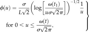4.2

where t₁ is the time when the census is taken.

Probability distribution (4.1)–(4.2) is shown in figure 7a. For a more general case of a multi-peak distribution, i.e. equation (3.1) with p > 1, the analytical expression for the pdf is not available but it can be readily obtained by numerical simulations; an example is shown in figure 7b. Therefore, in both cases the pdf has a bimodal shape, this shape being more pronounced on the single peak case.

Figure 7.

(a) Probability density function of sample values in a census in the case where the spatial distribution is single-peaked (cf. equation (3.1) with p = 1) as described by the probability density function (4.1) and (4.2). (b) Frequency Q of sample values in the case of a multi-peaked distribution (equation (3.1) with p = 4 and ω(t) = 1) obtained numerically.

We mention here that the frequency distribution shown in figure 7 is not unrealistic: the distribution of sample data observed in the population census of some plant species has a similar shape [49]. Yet it gives only one possible case from a great multiplicity of various probability distribution functions that are used to describe sampling data collected for different species and under different ecological conditions [50,51]. Questions therefore arise as to (i) how common is the situation where synchronization remains undetected on a coarse sampling grid and (ii) how the minimum number of samples sufficient to reveal synchronization may depend on the properties of the population dynamics as reflected by the pdf of the sampling data. Indeed, as was discussed in §2, the accuracy of the estimate of the average population density (2.1) depends on the sample size N. However, the accuracy of the estimate depends also on the way in which the sample values are distributed, because the rate of convergence of the arithmetic average to the true mean density can be somewhat different for different probability distributions. Therefore, the same sample size N may be sufficient to reveal synchronization in one case, e.g. for one probability distribution of sample values, but insufficient in case of another probability distribution.

To address these issues, in this section we simulate sampling data using a variety of probability density functions (table 1). We assume that the distance between any two neighbouring nodes of the sampling grid is large enough to exclude possible interference between them. Correspondingly, the population densities obtained at any two grid nodes in both domains A and B are independent identically distributed random variables drawn from a given pdf ϕ. This produces a certain spatial pattern of the population distribution which is somewhat different for different pdfs of the sampling data (e.g. having different variance) (figure 8). For a given ϕ, the procedure is repeated to generate the two time courses of the spatial patterns, i.e. in domains A and B. The correlation coefficient is then calculated basing on the time series of mean population density where the mean density is calculated as the arithmetic average over N samples taken in the corresponding census (equations (2.1)–(2.3)). For the same sequence of the generated spatial patterns, this procedure is repeated on sampling grids with different number of nodes to obtain ρ_ϕ(N).

Table 1.

Population models to describe frequency of sample values u in a census.

name	probability P{u=n} or probability density ϕ(u)	distribution parameter(s)	mean,
Poisson		λ	λ
exponential		λ
gamma		λ, m	mλ
lognormal		σ, μ
power law	C=(m−1)δ(m−1)	δ, m (m > 1)	, m > 2

Figure 8.

Spatial population distribution obtained on a hypothetical rectangular sampling grid of 10 × 10 = 100 nodes with the grid step Δx = Δy = 10 for (a) Poisson distribution of the population density, (b) exponential distribution of the population density. In both cases, the average density is . Note that different distributions of sampling data correspond to somewhat different spatial patterns, in particular, the variance of the spatial distribution is 10 and 100 for panels (a) and (b), respectively. (Online version in colour.)

To place our analysis into the context of a real field study, we relate the problem of spatial sampling to the recent study on synchronization of Tipula paludosa in agricultural landscape [15]. The metapopulation of T. paludosa was monitored for 15 years in 38 agricultural fields across southwest Scotland. In each of those fields, the T. paludosa population was subjected to annual census in winter, i.e. at the time when it is at the larvae stage and is mostly dwelling in the soil. In each field, 25 soil cores were taken at randomly chosen locations (cf. [12]). The number of larvae in each soil core was counted. Given the known radius r of the core, the count n provides a reliable index of the local population abundance; in particular, it can be used to calculate the local population density u as u = n/(πr²). The arithmetic average of the counts was then calculated for each field and each census. The 15 year courses of the population density obtained for each field were then fed pairwise into equations (2.2) and (2.3) to calculate the correlation coefficient ρ. It was observed that some of the fields are strongly synchronized, with ρ ≈ 0.8 or larger (for details see [15]).

For the purposes of our analysis, we choose two pairs of fields so that Pair 1 consists of fields A1 and B1 and Pair 2 consists of fields A2 and B2 (table 2). Figure 9 shows the corresponding time courses of the spatially average population counts. It is readily seen that the population fluctuations are not independent; indeed, the calculated correlation coefficient (table 2) shows that they are strongly correlated. The question that we are asking here is: how the conclusions about T. paludosa synchronization might have changed if the number of the samples (soil cores) would be much less than N = 25, could the synchronization still be seen? Similarly, if the number of samples would have been much larger than N = 25, would the results possibly reveal even stronger correlation between the fields?

Table 2.

Two pairs of fields from [15] used in our correlation modelling.

name (as used in the text)	position (grid reference)	max/min population count	course average, μ (count)	correlation coefficient, ρ (A,B)
A1	NS 111703	32/1	8.2	0.884
B1	NY 049748	22/0	4.73
A2	NN 943236	8/0	2.33	0.808
B2	NS 412331	27/0	6.6

Figure 9.

The average population counts over time in the selected pairs of correlated fields (see table 2). (a) Pair 1, crosses for A1, diamonds for B1; (b) Pair 2, crosses for A2, diamonds for B2. (Online version in colour.)

Unfortunately, the raw data, i.e. the insect counts for each soil core, are not available. In each census, only the arithmetic average of the samples is available for each field. It is therefore not possible to work with the original data, in particular, it not possible to tell what was the probability distribution for the sampling data (i.e. larvae counts). It was shown in [15] that the average density⁴ is well described by a lognormal distribution but this does not necessarily mean that the individual counts are distributed lognormally. To fill in for the missing information, we are going to replace the original sampling data with simulated data using different population models, i.e. different pdfs of the frequency of the sample values given in table 1. For each year of the survey, we simulate N_max samples to reproduce the actual (observed) average:

4.3

where the superscript ϕ refers to one of the models in table 1, s₁,…,s_Nmax are the samples generated according to a given pdf ϕ, and is the known average (figure 9). N_max is chosen to be sufficiently large to ensure that the arithmetic mean approaches closely its theoretical limiting value. (In simulations shown below, we used N_max = 100.) We then use only a subset N of these simulated samples, N ≤ N_max, to calculate the corresponding subset average:

4.4

Obviously, in a general case , because the estimation on a coarser sampling grid is less accurate. The average (4.4) is then used to calculate the correlation coefficient (2.2). By varying N, we reveal the dependence of ρ on the sample size N for any given pdf ϕ.

The results obtained for different population models as given by different pdfs in table 1 are shown in figures 10 and 11, where the columns (a,c,e) and (b,d,f) correspond to Pair 1 and Pair 2, respectively. Note that, for any given pdf ϕ, for each year in the time course the parameter(s) of the pdf are chosen somewhat differently in order to agree with the current value of ; see the last column in table 1. Given the random nature of the simulated samples and the relatively short length of the time courses (15 annual surveys, i.e. 15 points), it is not surprising that the correlation coefficient ρ exhibits stochastic fluctuations. To decrease the effect of stochasticity and hence to make the general tendency clearer, for any given N the procedure was repeated 10 times; the thick curve shows ρ(N) averaged over those ten realizations. To show the range of possible values due to the inherent randomness of the system, the confidence interval is calculated: the dotted curves show the averaged value of ρ plus–minus the standard deviation calculated over the 10 realizations.

Figure 10.

Correlation coefficient ρ(N) (thick curve) calculated for different population models and parameters (as in table 1): (a,b) Poisson distribution with , (c,d) gamma distribution with m=2 and , (e,f) lognormal distribution with σ = 0.45 and . Column (a,c,e) for Pair 1, column (b,d,f) for Pair 2. Dotted curves show the calculated value of ρ±standard deviation, the vertical distance between the curves thus being the confidence interval; the dashed-and-dotted line shows the true value of ρ.

Figure 11.

Correlation coefficient ρ(N) (thick curve) calculated for different population models and parameters (as in table 1): (a,b) exponential distribution with , (c,d) power law with m = 3 and , (e,f) power law with m = 2, in this case δ is chosen for to coincide with the median of the distribution. Column (a,c,e) for Pair 1, column (b,d,f) for Pair 2. Dotted curves show the calculated value of ρ±standard deviation, the vertical distance between the curves thus being the confidence interval; the dashed-and-dotted line shows the true value of ρ.

It is readily seen from figures 10 and 11 that there is a clear difference between the case where the probability distribution has a maximum at some positive value u > 0 (as for the Poisson, gamma and lognormal distributions) and the case where the probability distribution has a maximum at u = 0 (as for the exponential and power-law distributions). In the former case (figure 10), a good estimate of the correlation coefficient (e.g. within 10% of its true value shown by the dashed-and-dotted horizontal line) is typically obtained for a relatively small number of samples; in particular, just three to four samples per census can be sufficient for the Poisson and lognormal distributions and 9–10 in case of the gamma distribution. The situation is different in the latter case (figure 11). In the cases of the exponential distribution and the power law with m = 3, a reliable estimate of the true value of ρ is not obtained until the number of samples in a census is 18–20 (figure 11a–d). The convergence of ρ(N) to its true value is somewhat slower when the distribution of sample values is described by a power law with m = 2 where a reliable estimate is not obtained until the sample size N ≈ 25 (figure 11e). Interestingly, some apparently minor details of the dynamics can affect the results too: the required sample size appears to be smaller in Pair 2 than in Pair 1 for all three cases shown in figure 11.

5. Ghost synchronization on a coarse sampling grid

We therefore have shown that, when the population density exhibits considerable variation over space and the data are collected on a coarse sampling grid, synchronization is often lost as the correlation coefficient is usually much smaller than its actual value. In this section, we are going to demonstrate that the opposite is also possible. Namely, we will show that sampling on a coarse grid may result in a ‘ghost synchronization’, i.e. in the situation where the correlation coefficient calculated from the coarse sampling data has a value close to one whilst the dynamics is actually anti-correlated.

We consider a simple system consisting of two one-dimensional domains A and B where the population of a certain species has a unimodal spatial distribution with the maximum at the domain boundary:

5.1

Note that, although the functional form (5.1) of the population distribution is specific, the case where the population density decays monotonically with the distance from the domain border is relatively common in ecosystems and agroecosystems; in particular, it may correspond to the invasion of a pest insect to a farm field from adjoining uncultivated areas [52].

We assume that the populations are affected by factors that are different in the two domains, so that the population size in domain A and domain B evolves differently with time (but preserving the shape of the spatial distribution). We consider the following hypothetical situation:

5.2

where t ≥ 0 and a, b, γ, ω₀ and σ₀ are parameters. Since ω_A(0) = ω_B(0) = ω₀ and σ_A(0) = σ_B(0) = σ₀, the initial population distribution is the same in both domains. However, the dynamics is different: the maximum population density grows in domain A but decays in domain B while the width of the patch does not change in domain A but increases in domain B.

Let us consider the case where in both domains the initial distribution is aggregated in the vicinity of the habitat boundary, . If, for the sake of simplicity, we restrict our analysis to the time when the tail of the distribution at the right-hand side of the domains is still thin, i.e.  and , then the population size in domains A and B is, respectively, and . We then observe that the population size grows in domain A but decreases in domain B. Hence the dynamics is anti-correlated; the corresponding correlation coefficient must be negative, having a value close to −1. However, the population density at a given location does not necessarily behave in the same way. In fact, it is readily seen from the properties of function (5.1) that there is a sub-domain where the population density actually tends to increase simultaneously in both domains. An example is shown in figure 12. One can expect that, if the samples on the population density are taken in that sub-domain only, then the corresponding value of the correlation coefficient is going to be positive, possibly being close to one.

Figure 12.

Population density at the location x₁ = 10 (as given by equations (5.1) and (5.2) with parameters a = 0.5, b = 0.25, γ = 0.0001, ω₀ = 2 and σ₀ = 3) in domain A (curve 1) and in domain B (curve 2).

Having said that, it remains unclear how the correlation coefficient may depend on the number of samples and on their locations. To make a more quantitative insight into the properties of system (5.1) and (5.2), we now use simulations, i.e. we generate a sequence of sampling grids with different number of nodes N and calculate the correlation coefficient ρ(N) accordingly. To perform simulations, we use the following parameters: L_A = L_B = 300, a = 0.5, b = 0.25, γ = 0.0001, ω₀ = 2 and σ₀ = 3.

The results are shown in figure 13a,b where the sampling grid is chosen differently. In the case of figure 13a, in both domains A and B the additional nodes are added at the right, i.e. towards the tail of the spatial distribution, their location being defined as x_i = x₁+(i−1)Δx where 2 ≤ i ≤ N. The results shown in figure 13a are obtained in case Δx = x₁ = 10. We therefore observe that ρ is not very sensitive to the sample size N; the correlation coefficient changes just slightly from ρ (N = 1) ≈ 0.89 to ρ (N = 27) ≈ 1. Remarkably, these values have nothing to do with reality as the population dynamics described by equations (5.1) and (5.2) is anti-correlated with ρ ≈ −1.

Figure 13.

Dependence of the correlation coefficient on the number of nodes in the sampling grid for two different ways to refine the grid: (a) extra nodes are added towards the tail of the population spatial distribution, (b) extra nodes are added towards the maximum of the population spatial distribution; see the main text for more details.

In the case of figure 13b, in both domains A and B the additional nodes are added at the left, i.e. towards the centre of the spatial distribution (5.1). The location of additional nodes is defined as x_i = x₁−(i−1)Δx, 2 ≤ i ≤ N (the results shown in figure 13b are obtained for x₁ = 10 and Δx = 1). In this case, ρ strongly depends on N by exhibiting a monotonic decay from the false value ρ (N = 1) ≈ 0.89 to the actual value ρ (N = 10) ≈ −1.

We therefore conclude that, in order to obtain the correct value of the correlation coefficient, not only is the number of nodes in the sampling grid important but their location too, the latter being determined by the properties of the spatial pattern. In particular, in the case of system (5.1) and (5.2), samples collected in the area close to the maximum of the distribution are apparently more important as they bring more information than samples collected in the area at its tail. This conclusion is further confirmed by the dependence ρ(N) calculated on a grid with mixed properties (figure 14) where the second node is placed in the ‘important’ range 0 < x < x₁, namely at the location x₂ = 0.5x₁, but other additional nodes are added at the right of x₁ with the spatial step Δx=0.5x₁. It is readily seen that, while the second node brings some essential information sufficient to change the value of the correlation coefficient from a completely false value ρ ≈ 0.89 to a much more realistic ρ ≈ −0.85, all other nodes added in the area towards the distribution tail do not improve the accuracy any further.

Figure 14.

Correlation coefficient ρ(N) in the case where the sampling grid is refined in a mixed way; see the main text for details.

6. Discussion and conclusion

In ecological and environmental studies as well as in other natural sciences and environmental engineering, it is often needed to estimate the population size of a given species or the total mass of a given substance based on local, spatially discrete data collected at the nodes of a certain sampling grid [1–4,7]. When the spatial distribution of a given population (or substance) exhibits a considerable variability in space, which is rather typical in ecology [25,43,53–56] and agroecology [13,36,37,57], the number of collected samples may not always be sufficient to resolve the details of the spatial configuration. Moreover, information about the spatial pattern of the population density distribution, e.g. the exact location of peaks or patches, usually is not known a priori (but see [13]); it is eventually obtained as a result of the analysis of the sampling data [49].

It therefore often happens that the number of samples in a census as well as the location of samples are chosen based on a guess or a certain rule of thumb. It can also be negatively affected by some external constraints, e.g. a limited budget. As a result, the sampling grid may appear to be coarse, i.e. not resolving the spatial population distribution in sufficient details. Estimation of the population size⁵ on a coarse grid would normally have low accuracy [3,6,14,21,22,27] or could even become probabilistic [28,58]. When the estimated population size is used as the input information for some further analysis, e.g. to assess the correlation strength between two habitats, this inaccuracy is likely to affect the results. In this paper, we showed that the correlation coefficient ρ calculated based on sampling data collected over a coarse grid often has little to do with its true value. Even a very strong correlation (i.e. 0.8 ≤ ρ ≤ 1), usually referred to as synchronization, can be ‘lost’, i.e. remain unseen, as the value obtained on a coarse grid is typically ρ ∼ 0.5 or less (e.g. figures 4–6 and 11). Moreover, we also showed that, when the location of nodes in the sampling grid is chosen inadequately, the opposite case is possible, i.e. the correlation coefficient calculated based on the sampling data is close to one while in reality there is no synchronization (see §5). Remarkably, this ‘ghost synchronization’ can happen even if the sampling grid contains an apparently large number of nodes (e.g. figure 13a).

Here, we mention that synchronization has a variety of implications for ecology, agroecology and nature conservation, in particular because synchronization is one of the main dynamical mechanisms behind large-scale population crashes [18,23] as well as large-scale outbreaks [29,41]. Hence, the capability to detect the presence or the absence of synchronization is crucial for planning, forecasting and decision-making. Reliability of the calculated value of the correlation coefficient is therefore an issue of high practical importance.

6.1. Test of grid coarseness

An important question arises as to whether it may be possible, based on the available sampling data, to separate the cases where the calculated ρ is likely to be close to its true value from the cases where the calculated ρ is likely to be wrong. Based on the results of our analysis in §4, the following test of grid coarseness can be suggested. We do not normally know the spatial pattern but we can estimate, based on the collected data, the pdf of the sampling data. Once the pdf is revealed, additional data distributed accordingly to this pdf can easily be simulated to create a virtual sequence of sampling grids with different number of nodes N, and then ρ(N) can be calculated following the procedure described in §4. Once ρ(N) is available, its convergence to the large-N limit can be readily established and then it is straightforward to estimate from the shape of the graph how many nodes are needed. For instance, in the case of the Poisson distribution (figure 10a,b), a sparse grid consisting of four to five nodes should be sufficient to obtain the true value of the correlation coefficient; however, in case of the exponential distribution the grid will only become sufficiently refined when the number of nodes is 30 or more (cf. figure 11a).

With this new understanding thus achieved, we are now going to briefly revisit some cases of synchronization reported in the literature with the purpose to assess whether the corresponding sampling grids were adequate or perhaps too coarse:

• — Region-wide synchronization of Tipula paludosa in southwest Scotland was reported in [15]. The average population density in each farm field used in the study was estimated based on 25 samples (soil cores). Moreover, there was some evidence presented that the distribution of frequencies was well described by a lognormal distribution [15]. An inspection of figure 10e,f reveals that ρ(N) approaches the vicinity of its true value (with the 10% tolerance) when N ≥ 4. We therefore conclude that the results reported in [15] are reliable.

• — Synchronization of several Lepidoptera species was observed in central Appalachian deciduous forests [32]. The study included twelve plots, each of them having the same area of 200 ha. In each plot, the data were collected by a single light trap. Raimondo et al. [32] do not provide any information about the frequency distribution of their sampling data. However, in another study on Lepidoptera [59], it was shown that sampling data for at least some Lepidoptera species are well described by either negative binomial distribution or Poisson distribution [59]. If we assume that this result is transferrable between the two studies (which is a rather strong assumption, because the study [59] was done in another geographical region), then we can make use of the results shown in figure 10a,b. It is then readily seen that a single sample (i.e. single trap) is very unlikely to provide an exact value of ρ as the true value does not even fall into the range of possible values (shown by the dotted curves). The estimate of the correlation coefficient obtained based on a single sample is likely to considerably underestimate its true value, with the deviation from the true value being about 20–25%. We therefore conclude that Lepidoptera species in Appalachian forests are likely to be correlated much stronger than was observed in [30].

• — Synchronization of carabid beetles due to the weather fluctuations (the phenomenon known as the Moran effect [32–34]) was observed in a study performed in a nature reserve in The Netherlands [35]. The study area covering a few square kilometres was split into a few zones and in each zone three pitfall traps were installed to sample the carabid beetle population. Baars & Van Dijk [35] did not provide any analysis of the frequency distribution of their sampling data (i.e. trap counts). Some relevant information is available from another study on carabid beetles performed in the same geographical region [56,60]. Although Rossi et al. [60] did not do a formal fitting of the trap count data with a statistical model, the shape of the frequency histogram (e.g. fig. 3 and 6 in [60]) suggests that it is likely to be better described by a probability density function with the maximum at the origin and a relatively slow rate of decay at the tail. We therefore hypothesize that, from the cases analysed in §4, either the exponential distribution or a power-law distribution are best candidates. We should also mention here the apparent visual similarity between the qualitative properties of the field data on carabid beetle distribution shown in figure 1b and the simulated spatial pattern shown in figure 8b, the latter being obtained using the exponential distribution. Making use of the results shown in figure 11a,b, we readily observe that the sampling grid consisting of three nodes is coarse and is likely to considerably underestimate the actual strength of the correlation. This may be a reason why the correlation between different sites and/or different subpopulations reported by Baars & Van Dijk [35] was not as strong and widespread as it perhaps might intuitively be expected.

6.2. Concluding remarks

We therefore conclude that the properties of the sampling grid such as the total number of samples in a survey and their location must be decided based upon a rigorous argument rather than a guess or rule of thumb. Although this may sound as a trivial statement, in field studies focusing on revealing synchronization surprisingly little attention is paid to checking whether the number of samples (e.g. traps) is sufficient to provide a robust estimate of the population abundance. As just one example, here we cite Baars & Van Dijk [35]: ‘summed catches were assumed to represent the adult density around a series of pitfall traps’.⁶ As we discussed above, one rigorous argument could be based on the analysis of the sampling data frequencies which makes it possible to estimate the minimum required number of nodes in the grid. Where possible, this should also be combined with some a priori knowledge of typical properties of the spatial population distribution of the given species. For instance, this information can be obtained from relevant previous studies (e.g. as available from the literature) or from a specially designed pilot study. Although it undoubtedly requires an extra effort, it seems to be a necessary step in order to make any conclusion on the presence or absence of synchronization reliable. In particular, in order to avoid the ‘ghost synchronization’, one should have some a priori knowledge of the population dynamics of the species. This should include not only the pattern of the population spatial distribution, but also some information about the temporal scales of the dynamics. For instance, if the correlation coefficient in the model (5.1) and (5.2) is calculated using time courses obtained over much longer time, then the correct value ρ (N) ≈ −1 can be obtained even for a relatively small N (for the sake of brevity, we do not show the results here).

One important message following from our study is that the spatial resolution of the sampling grid cannot be decided upon based on just one universal rule. The appropriate frequency of spatial sampling appears to be context-specific and hence depends on the focus of the study. For instance, if the focus is on revealing the details of population distribution across all scales of spatial variability, then the approach based on the Nyquist frequency is known to work well: in order to avoid information loss, it recommends to have at least two sampling nodes per peak in the smallest spatial scale involved [25,44]. (We mention here that in the problem of ecological patterning relevant spatial scales range from the microscale of the size of an individual to the macroscale of the geographical and climatic variation [61], and hence the decision about the ‘minimum’ spatial scale may often be arguable.) However, if the focus is on the evaluation of the total population size, the requirements to the sampling grid can be much less restrictive as the resolution depends on the required accuracy [28,42,58]. Furthermore, in case sampling is needed not only across space but also over time, e.g. to reveal the presence or the absence of synchronization, the sampling grid resolution strongly depends on the population dynamics of the sampled species so that the required number of nodes in a given spatial domain can differ by an order of magnitude (cf. figures 10a and 11a). For this problem, the Nyquist frequency is hardly relevant at all.

Our study leaves a few open questions. Perhaps the most challenging one is about the ghost synchronization. In this paper, we have identified only one case where this curious artefact can happen if samples are collected on a coarse grid, i.e. where the population density in the corresponding domains decreases monotonically away from a domain boundary, provided the properties of this density profile changes with time in a certain way. It remains unclear whether the ‘ghost synchronization’ is an exotic situation only happening under some specific conditions or it happens more commonly. This should become a focus of a separate study. Another highly practical issue is the effect of the environmental heterogeneity. Throughout this paper, we have assumed that all sampling locations over the given domain are equivalent, in particular, assuming that the probability density function of the sampling data is the same at any location. In real ecosystems, this is not always the case. Further development of our approach to include the effects of spatial heterogeneity will be a focus of future research.

Data accessibility

All field data that are used or mentioned in our study are taken from the literature and hence freely available.

Authors' contributions

N.P. and S.P. contributed equally to conceiving and performing the study; N.P. and S.P. wrote the manuscript; N.P. and S.P. approved the publication of the manuscript in its current form.

Competing interests

We declare that we have no competing interests.

Funding

We received no funding for this study.

References

- 1.Benjamin MM, Lawler DF. 2013. Water quality engineering: physical & chemical treatment processes. New York, NY: John Wiley & Sons. [Google Scholar]
- 2.Boissonnat J-D, Nullans S. 1996. Reconstruction of geological structures from heterogeneous and sparse data. INRIA Report N3069.
- 3.Seber GA. 1982. The estimation of animal abundance and related parameters. London, UK: Charles Griffin. [Google Scholar]
- 4.Wu Q, Xu H, Zou X. 2005. An effective method for 3D geological modeling with multi-source data integration. Comput. Geosci. 31, 35–43. ( 10.1016/j.cageo.2004.09.005) [DOI] [Google Scholar]
- 5.Eppstein MJ, Hawrysz DJ, Godavarty A, Sevick-Muraca EM. 2002. Three-dimensional, Bayesian image reconstruction from sparse and noisy data sets: near-infrared fluorescence tomography. Proc. Natl Acad. Sci. USA 99, 9619–9624. ( 10.1073/pnas.112217899) [DOI] [PMC free article] [PubMed] [Google Scholar]
- 6.Petrovskii SV, Petrovskaya N, Bearup D. 2014. Multiscale approach to pest insect monitoring: random walks, pattern formation, synchronization, and networks. Phys. Life Rev. 11, 467–525. ( 10.1016/j.plrev.2014.02.001) [DOI] [PubMed] [Google Scholar]
- 7.Sutherland WJ. (ed.) 1996. Ecological census techniques: a handbook. Cambridge, UK: Cambridge University Press. [Google Scholar]
- 8.Bakus GJ. et al. 2007. A comparison of some population density sampling techniques for biodiversity, conservation, and environmental impact studies. Biodiv. Conserv. 16, 2445–2455. ( 10.1007/s10531-006-9141-7) [DOI] [Google Scholar]
- 9.Noss RF. 1990. Indicators for monitoring biodiversity: a hierarchical approach. Conserv. Biol. 4, 355–364. ( 10.1111/j.1523-1739.1990.tb00309.x) [DOI] [Google Scholar]
- 10.Engler R, Guisan A, Rechsteiner L. 2004. An improved approach for predicting the distribution of rare and endangered species from occurrence and pseudo-absence data. J. Appl. Ecol. 41, 263–274. ( 10.1111/j.0021-8901.2004.00881.x) [DOI] [Google Scholar]
- 11.Sudman S, Sirken MG, Cowan CD. 1988. Sampling rare and elusive populations. Science 240, 991–996. ( 10.1126/science.240.4855.991) [DOI] [PubMed] [Google Scholar]
- 12.Blackshaw RP. 1983. The annual leatherjacket survey in Northern Irealnd, 1965–1982, and some factors affecting populations. Plant Path. 32, 345–349. ( 10.1111/j.1365-3059.1983.tb02843.x) [DOI] [Google Scholar]
- 13.Alexander CJ, Holland JM, Winder L, Wooley C, Perry JN. 2005. Performance of sampling strategies in the presence of known spatial patterns. Ann. Appl. Biol. 146, 361–370. ( 10.1111/j.1744-7348.2005.040129.x) [DOI] [Google Scholar]
- 14.Boag B, Deeks L, Orr A, Neilson R. 2005. A spatio-temporal analysis of a New Zealand flatworm (Arthurdendyus triangulatus) population in western Scotland. Ann. Appl. Biol. 147, 81–88. ( 10.1111/j.1744-7348.2005.00017.x) [DOI] [Google Scholar]
- 15.Bearup D, Petrovskii SV, Blackshaw R, Hastings A. 2013. The impact of terrain and weather conditions on the metapopulation of Tipula paludosa in South-Western Scotland: linking pattern to process. Am. Nat. 182, 393–409. ( 10.1086/671162) [DOI] [PubMed] [Google Scholar]
- 16.Hanski I, Woiwod IP. 1993. Spatial synchrony in the dynamics of moth and aphid populations. J. Anim. Ecol. 62, 656–668. ( 10.2307/5386) [DOI] [Google Scholar]
- 17.Peltonen M, Liebhold A, Bjørnstad ON, Williams DW. 2002. Variation in spatial synchrony among forest insect species: roles of regional stochasticity and dispersal. Ecology 83, 3120–3129. ( 10.1890/0012-9658(2002)083%5B3120:SSIFIO%5D2.0.CO;2) [DOI] [Google Scholar]
- 18.Sutcliffe OL, Thomas CD, Yates TJ, Greatorex-Davies JN. 1997. Correlated extinctions, colonizations and population fluctuations in a highly connected ringlet butterfly metapopulation. Oecologia 109, 235–241. ( 10.1007/s004420050078) [DOI] [PubMed] [Google Scholar]
- 19.Williams DW, Liebhold AM. 1995. Influence of weather on the synchrony of gypsy moth (Lepidoptera: Lymantriidae) outbreaks in New England. Environ. Entomol. 24, 987–995. ( 10.1093/ee/24.5.987) [DOI] [Google Scholar]
- 20.Pedigo LP, Buntin GD (eds). 1994. Handbook of sampling methods for arthropods in agriculture. Boca Raton, FL: CRC Press. [Google Scholar]
- 21.Petrovskaya NB, Petrovskii SV. 2010. The coarse-grid problem in ecological monitoring. Proc. R. Soc. A 466, 2933–2953. ( 10.1098/rspa.2010.0023) [DOI] [Google Scholar]
- 22.Petrovskaya NB, Petrovskii SV, Murchie AK. 2012. Challenges of ecological monitoring: estimating population abundance from sparse trap counts. J. R. Soc. Interface 9, 420–435. ( 10.1098/rsif.2011.0386) [DOI] [PMC free article] [PubMed] [Google Scholar]
- 23.Milne A, Laughlin R, Coggins RE. 1965. The 1955 and 1959 population crashes of the leatherjacket, Tipula paludosa Meigen, in Northumberland. J. Anim. Ecol. 34, 529–534. ( 10.2307/2447) [DOI] [Google Scholar]
- 24.Petrovskii SV, Bearup D, Ahmed DA, Blackshaw R. 2012. Estimating insect population density from trap counts. Ecol. Compl. 10, 69–82. ( 10.1016/j.ecocom.2011.10.002) [DOI] [Google Scholar]
- 25.Platt T, Denman KL. 1975. Spectral analysis in ecology. Annu. Rev. Ecol. Syst. 6, 189–210. ( 10.1146/annurev.es.06.110175.001201) [DOI] [Google Scholar]
- 26.Taylor LR, Woiwod IP, Perry JN. 1978. The density-dependence of spatial behaviour and the rarity of randomness. J. Anim. Ecol. 47, 383–406. ( 10.2307/3790) [DOI] [Google Scholar]
- 27.Boag B, Mackenzie K, McNicol JW, Neilson R. 2010. Sampling for the New Zealand flatworm. Proc. Conf. on Crop Protection in Northern Britain 2010, Dundee, UK, 23–24 February 2010, pp. 45–50. [Google Scholar]
- 28.Petrovskaya N, Embleton N. 2013. Evaluation of peak functions on ultra-coarse grids. Proc. R. Soc. A 469, 20120665 ( 10.1098/rspa.2012.0665) [DOI] [Google Scholar]
- 29.Liebhold A, Koenig WD, Bjornstad ON. 2004. Spatial synchrony in population dynamics. Annu. Rev. Ecol. Evol. Syst. 35, 467–490. ( 10.1146/annurev.ecolsys.34.011802.132516) [DOI] [Google Scholar]
- 30.Raimondo S, Liebhold AM, Strazanac JS, Butler L. 2004. Population synchrony within and among Lepidoptera species in relation to weather, phylogeny, and larval phenology. Environ. Entomol. 29, 96–105. ( 10.1111/j.0307-6946.2004.00579.x) [DOI] [Google Scholar]
- 31.Ranta E, Kaitala V, Lindstrom K, Helle E. 1997. Moran effect and synchrony in population dynamics. Oikos 78, 136–142. ( 10.2307/3545809) [DOI] [Google Scholar]
- 32.Moran PAP. 1953. The statistical analysis of the Canadian lynx cycle. I. Structure and prediction. Aust. J. Zool. 1, 163–173. ( 10.1071/ZO9530163) [DOI] [Google Scholar]
- 33.Moran PAP. 1953. The statistical analysis of the Canadian lynx cycle. II. Synchronization and meterology. Austr. J. Zool. 1, 291–298. ( 10.1071/ZO9530291) [DOI] [Google Scholar]
- 34.Royama T. 1992. Analytical population dynamics. New York, NY: Chapman & Hall. [Google Scholar]
- 35.Baars MA, Van Dijk TS. 1984. Population dynamics of two carabid beetles at a Dutch heathland. I. Subpopulation fluctuations in relation to weather and dispersal. J. Anim. Ecol. 53, 375–388. ( 10.2307/4522) [DOI] [Google Scholar]
- 36.Lyles D, Rosenstock TS, Hastings A, Brown PH. 2009. The role of large environmental noise in masting: general model and example from pistachio trees. J. Theor. Biol. 259, 701–713. ( 10.1016/j.jtbi.2009.04.015) [DOI] [PubMed] [Google Scholar]
- 37.Rosenstock TS, Hastings A, Koenig WD, Lyles DJ, Brown PH. 2011. Testing Moran's theorem in an agroecosystem. Oikos 120, 1434–1440. ( 10.1111/j.1600-0706.2011.19360.x) [DOI] [Google Scholar]
- 38.Bearup D, Benefer CM, Petrovskii SV, Blackshaw R. 2016. Revisiting Brownian motion as a description of animal movement: a comparison to experimental movement data. Methods Ecol. Evol. 7, 1525–1537. ( 10.1111/2041-210X.12615) [DOI] [Google Scholar]
- 39.Byers JA. 1993. Simulation and equation models of insect population control by pheromone-based traps. J. Chem. Ecol. 19, 1939–1956. ( 10.1007/BF00983798) [DOI] [PubMed] [Google Scholar]
- 40.Evans JD. 1996. Straightforward statistics for the behavioral sciences. Pacific Grove, CA: Brooks/Cole Publishing. [Google Scholar]
- 41.Swetnam TW, Lynch AM. 1993. Multicentury, regional scale patterns of Western spruce budworm outbreaks. Ecol. Monogr. 63, 399–424. ( 10.2307/2937153) [DOI] [Google Scholar]
- 42.Petrovskaya NB, Embleton NL. 2014. Computational methods for accurate evaluation of pest insect population size. In Ecological modelling applied to entomology (eds WAC Godoy, CP Ferreira), pp. 171–218. Berlin, Germany: Springer. [Google Scholar]
- 43.Malchow H, Petrovskii SV, Venturino E. 2008. Spatiotemporal patterns in ecology and epidemiology: theory, models, and simulations. Boca Raton, FL: CRC Press. [Google Scholar]
- 44.Denny MW, Helmuth B, Leonard GH, Harley CDG, Luke JH, Hunt LJH, Nelson EK. 2004. Quantifying scale in ecology: lessons from a wave-swept shore. Ecol. Monogr. 74, 513–532. ( 10.1890/03-4043) [DOI] [Google Scholar]
- 45.Balescu R. 1975. Equilibrium and nonequilibrium statistical mechanics. New York, NY: John Wiley. [Google Scholar]
- 46.Ricker WE. 1954. Stock and recruitment. J. Fish. Res. Board Can. 11, 559–623. ( 10.1139/f54-039) [DOI] [Google Scholar]
- 47.Toft JE. 2013. From mountains to sound: modelling the sensitivity of Dungeness crab and Pacific oyster to land-sea interactions in Hood Canal, WA. ICES J. Mar. Sci. 71, 725–738. ( 10.1093/icesjms/fst072) [DOI] [Google Scholar]
- 48.Allman ES, Rhodes JA. 2004. Mathematical models in biology: an introduction. Cambridge, UK: Cambridge University Press. [Google Scholar]
- 49.Damgaard C. 2009. On the distribution of plant abundance data. Ecol. Inform. 4, 76–82. ( 10.1016/j.ecoinf.2009.02.002) [DOI] [Google Scholar]
- 50.Bolker BM. 2008. Ecological models and data in R. Princeton, NJ: Princeton University Press. [Google Scholar]
- 51.Young LJ, Young J. 1998. Statistical ecology. Berlin, Germany: Springer. [Google Scholar]
- 52.Bearup D, Petrovskaya N, Petrovskii SV. 2015. Some analytical and numerical approaches to understanding trap counts resulting from pest insect immigration. Math. Biosci. 263, 143–160. ( 10.1016/j.mbs.2015.02.008) [DOI] [PubMed] [Google Scholar]
- 53.Davis MB, Calcote RR, Sugita S, Takahara H. 1998. Patchy invasion and the origin of a Hemlock-Hardwoods forest mosaic. Ecology 79, 2641–2659. ( 10.2307/176507) [DOI] [Google Scholar]
- 54.Grünbaum D. 2012. The logic of ecological patchiness. Interface Focus 2, 150–155. ( 10.1098/rsfs.2011.0084) [DOI] [PMC free article] [PubMed] [Google Scholar]
- 55.Levin S. 1994. Patchiness in marine and terrestrial systems: from individuals to populations. Phil. Trans. R. Soc. B 343, 99–103. ( 10.1098/rstb.1994.0013) [DOI] [Google Scholar]
- 56.Hengeveld R. 1979. The analysis of spatial patterns of some ground beetles (col. Carabidae). In Spatial and temporal analysis in ecology (eds M Cormack, JK Ord), pp. 333–346. Fairland MD: International Co-operative Publishing House. [Google Scholar]
- 57.Holland JM, Perry JN, Winder L. 1999. The within-field spatial and temporal distribution of arthropods in winter wheat. Bull. Entomol. Res. 89, 499–513. ( 10.1017/S0007485399000656) [DOI] [Google Scholar]
- 58.Petrovskaya NB. Submitted ‘Catch me if you can’: evaluating the population size in the presence of a spatial pattern. [Google Scholar]
- 59.Clarke-Harris D, Fleischer SJ. 2003. Sequential sampling and biorational chemistries for management of Lepidopteran pests of vegetable amaranth in the Caribbean. J. Econ. Entomol. 96, 798–804. ( 10.1093/jee/96.3.798) [DOI] [PubMed] [Google Scholar]
- 60.Rossi RE, Mulla DJ, Journel AG, Franz EH. 1992. Geostatistical tools for modeling and interpreting ecological spatial dependence. Ecol. Monogr. 62, 277–314. ( 10.2307/2937096) [DOI] [Google Scholar]
- 61.Petrovskii SV. 2016. Pattern, process, scale, and model's sensitivity: a comment. Phys. Life Rev. 19, 131–134. ( 10.1016/j.plrev.2016.09.003) [DOI] [PubMed] [Google Scholar]
Associated Data
This section collects any data citations, data availability statements, or supplementary materials included in this article.
Data Availability Statement