Abstract
Multi-fidelity modelling enables accurate inference of quantities of interest by synergistically combining realizations of low-cost/low-fidelity models with a small set of high-fidelity observations. This is particularly effective when the low- and high-fidelity models exhibit strong correlations, and can lead to significant computational gains over approaches that solely rely on high-fidelity models. However, in many cases of practical interest, low-fidelity models can only be well correlated to their high-fidelity counterparts for a specific range of input parameters, and potentially return wrong trends and erroneous predictions if probed outside of their validity regime. Here we put forth a probabilistic framework based on Gaussian process regression and nonlinear autoregressive schemes that is capable of learning complex nonlinear and space-dependent cross-correlations between models of variable fidelity, and can effectively safeguard against low-fidelity models that provide wrong trends. This introduces a new class of multi-fidelity information fusion algorithms that provide a fundamental extension to the existing linear autoregressive methodologies, while still maintaining the same algorithmic complexity and overall computational cost. The performance of the proposed methods is tested in several benchmark problems involving both synthetic and real multi-fidelity datasets from computational fluid dynamics simulations.
Keywords: Gaussian processes, uncertainty quantification, deep learning, Bayesian inference
1. Introduction
In recent years, we have been witnessing the emergence of a new wave in computational science where data-driven approaches are starting to take the centre stage. Among these developments, the concept of multi-fidelity modelling has been steadily gaining appeal among the computational science and engineering communities, as it allows one to use simple but potentially inaccurate models that carry a low computational cost, and effectively enhance their accuracy by injecting a small set of high-fidelity observations. By exploiting the cross-correlations between the low- and high-fidelity data via machine learning, this procedure can lead to significant computational gains and allow us to address problems that would be impossible to tackle if we solely relied on computationally demanding high-fidelity models. A non-exhaustive review on multi-fidelity modelling approaches with a particular focus on the areas of uncertainty propagation, inference and optimization was recently given by Peherstorfer et al. [1]. Other representative studies that highlight the merits and success of multi-fidelity models in areas including design, model inversion and uncertainty quantification can be found in [2–4].
Many of these multi-fidelity approaches are based on Gaussian process (GP) regression [5] in combination with the linear autoregressive information fusion scheme put forth by Kennedy & O'Hagan [6]. Their success is well documented in cases where low-fidelity models can capture the right trends, and the low- and high-fidelity model outputs exhibit strong linear correlation across the input space [2–4]. Moreover, by construction, in cases where such linear correlations cannot be detected during model training then the algorithm ignores the low-fidelity data and puts all the weight solely on the high-fidelity observations. Although this is a desirable feature, we later show that there exist cases where the low- and high-fidelity data exhibit more complex nonlinear and space-dependent cross-correlations that are very informative, but are inevitably ignored owing to the simple linear autoregressive structure assumed by the Kennedy and O'Hagan scheme. Such cases often arise in realistic modelling scenarios where low-fidelity models can typically be trusted and are well correlated to their high-fidelity counterparts only for a specific range of input parameters.
Take, for example, the case of multi-fidelity modelling of mixed convection flows past a cylinder using experimental correlations and direct numerical simulations as put forth in [7], and revisited in §3c of this paper. There, the low-fidelity experimental correlations stand true, and are strongly correlated with high-fidelity direct numerical simulations, in the case of aiding flows where the mixed-convection flow is steady and remains attached to the surface of the cylinder. However, this is far from true for the case of opposing flows where the dynamics become time dependent, and the low-fidelity models return erroneous trends and predictions that are off by up to 30% [7]. Such problems pose the question of designing flexible multi-fidelity algorithms that can learn more complex cross-correlations between data, safeguard against low-fidelity models that may provide wrong trends, but are also able to extract any informative behaviour from them.
The scope of this study is situated exactly at this junction. We revisit the classical autoregressive scheme of Kennedy and O'Hagan, and propose a fundamental extension that results in a new class of flexible and data-efficient multi-fidelity information fusion algorithms. Specifically, we adopt a functional composition approach inspired by deep learning, and derive a novel multi-fidelity scheme that is able to learn complex nonlinear and space-dependent cross-correlations between data, without sacrificing the algorithmic simplicity and overall computational cost of the Kennedy and O'Hagan approach.
2. Methods
(a). Regression with Gaussian processes
The main building block of our multi-fidelity modelling approach is GP regression and autoregressive stochastic schemes (see [5,6,8]). GP regression defines a supervised learning problem, in which we assume the availability of datasets comprising input/output pairs of observations of i=1,…,n that are generated by an unknown mapping f
| 2.1 |
The unknown function f(x) is typically assigned a zero mean GP prior, i.e. , where k is an appropriate kernel function parametrized by a vector of hyper-parameters θ that gives rise to a symmetric positive-definite covariance matrix Kij=k(xi,xj;θ), . The prior essentially assigns a measure for quantifying pairwise correlations between the input points (xi,xj) and reflects our prior knowledge on the properties of the function to be approximated (e.g. regularity, monotonicity, periodicity). Moreover, the eigenfunctions of the kernel define a reproducing kernel Hilbert space, which characterizes the class of functions that are within the approximation capacity of the predictive GP posterior mean [5].
The vector of hyper-parameters θ is determined by maximizing the marginal log-likelihood of the model (see [5]), i.e.
| 2.2 |
Assuming a Gaussian likelihood, the posterior distribution p( f|y,X) is tractable and can be used to perform predictive inference for a new output f*, given a new input x* as
| 2.3 |
| 2.4 |
| 2.5 |
where k*n=[k(x*,x1),…,k(x*,xn)] and k**=k(x*,x*). Predictions are computed using the posterior mean μ*, while uncertainty associated with these predictions is quantified through the posterior variance .
(b). Multi-fidelity modelling with recursive Gaussian processes
The GP regression framework can be systematically extended to construct probabilistic models that enable the combination of variable fidelity information sources (see [6,8]). To this end, suppose that we have s levels of information sources producing outputs yt(xt), at locations . We can organize the observed data pairs by increasing fidelity as , t=1,…,s. Then, ys denotes the output of the most accurate and expensive to evaluate model, whereas y1 is the output of the cheapest and least accurate model available. In this setting, the autoregressive scheme of [6] reads as
| 2.6 |
where ft−1 and ft are GPs modelling the data at fidelity level (t−1) and t, respectively, ρ is a scaling constant that quantifies the correlation between the model outputs {yt,yt−1} and δt(xt) is a GP distributed with mean μδt and covariance function kt, i.e. . This construction implies the Markov property
| 2.7 |
which translates into assuming that, given the nearest point ft−1(x), we can learn nothing more about ft(x) from any other model output ft−1(x′), for x≠x′ [9,6].
A numerically efficient recursive inference scheme can be constructed by adopting the derivation put forth by Le Gratiet & Garnier [8]. Specifically, this is achieved by replacing the GP prior ft−1(x) appearing in equation (2.6) with the GP posterior f*t−1(x) of the previous inference level, while assuming that the corresponding experimental design sets have a nested structure, i.e . In other words, this assumption implies that the training inputs of the higher fidelity levels need to be a subset of the training inputs of the lower fidelity levels. According to Le Gratiet & Garnier [8], this scheme is exactly matching the Gaussian posterior distribution predicted by the fully coupled scheme of Kennedy & O'Hagan [6]. However, now the inference problem is essentially decoupled into s standard GP regression problems, yielding the multi-fidelity posterior distribution p( ft|yt,Xt,f*t−1), t=1,…,s, with predictive mean and variance at each level given by
| 2.8 |
and
| 2.9 |
where nt denotes the number of training point locations where we have observed data from the t-th information source.
(c). Nonlinear information fusion algorithms
(i). General formulation
We generalize the autoregressive multi-fidelity scheme of equation (2.6) to
| 2.10 |
where zt−1(⋅) is an unknown function that maps the lower fidelity model output to the higher fidelity one. Here, we propose a Bayesian non-parametric treatment of z by assigning it a GP prior. Because ft−1 in equation (2.6) is also assigned a GP prior, the functional composition of two GP priors, i.e. zt−1(ft−1(x)), gives rise to the so-called deep GP as first put forth in [10,11], and, therefore, the posterior distribution of ft is no longer Gaussian. This general formulation allows us to go well beyond the linear structure of the Kennedy & O'Hagan [6] scheme, and enables the construction of flexible and inherently nonlinear and non-Gaussian multi-fidelity information fusion algorithms.
However, this generality comes at a price as the intractability of deep GPs introduces a training procedure that involves variational approximations, leading to a significant increase in computational cost and far more complex implementations than standard GP regression. Although great progress has been made in designing robust and efficient inference methods for such models [12,13], here we seek to harness their functionality without compromising the analytical tractability and favourable algorithmic complexity of standard GP regression. To this end, motivated by the approach put forth by Le Gratiet & Garnier [8], and outlined in §2b, we replace the GP prior ft−1 with the GP posterior from the previous inference level f*t−1(x). Then, using the additive structure of equation (2.10), along with the independence assumption between the GPs zt−1 and δt, we can summarize the autoregressive scheme of equation (2.10) as
| 2.11 |
where . The independence assumption between zt−1 and δt follows the construction of Kennedy & O'Hagan [6] and Le Gratiet & Garnier [8]. In our particular setting, the key implication is that, under this independence assumption, the δt process gets implicitly ‘absorbed’ into gt in equation (2.11). Moreover, under the assumption of noiseless data and stationary kernels, this leads to an equivalent Markov property as in equation (2.7), which translates into assuming that given the nearest point of the nonlinearly transformed lower fidelity level posterior, i.e. zt−1( f*t−1(x)), we can learn nothing more about ft(x) from any other model output zt−1( f*t−1(x′)), for x≠x′[9,6].
Essentially, this defines a (d+1)-dimensional map that jointly relates the input space and the outputs of the lower fidelity level to the output of the higher fidelity model. Note that, under the assumption of nested training sets (i.e. xt⊆xt−1) and noiseless observations {yt,yt−1}, the training of gt given the available data {xt,yt} reduces to a straightforward maximum-likelihood estimation problem since the posterior of the lower fidelity level evaluated at xt (i.e. f*t−1(xt)) is by construction a known deterministic quantity.
Although this scheme can serve as a launch pad for constructing flexible and expressive multi-fidelity information fusion algorithms, a first observation is that the chosen structure for the covariance function of gt may not be natural as the inputs f*t−1(x) and x belong to inherently different spaces. Here, we extend the proposed methodology by introducing a more structured prior for gt that better reflects the autoregressive nature of equation (2.6). To this end, we consider a covariance kernel that decomposes as
| 2.12 |
where ktρ, ktf and ktδ are valid covariance functions and {θtρ,θtf,θtδ} denote their hyper-parameters. The latter can be readily learnt from the data {xt,yt} via the maximum-likelihood estimation procedure described in §2a (see equation (2.2)) using the kernel ktg. In comparison with the recursive implementation of the classical Kennedy and O'Hagan scheme, our approach requires the estimation of (2d+3) instead of (d+3) model hyper-parameters, assuming that all kernels account for directional anisotropy in each input dimension using automatic relevance determination (ARD) weights [5]. However, this difference is considered negligible, especially when compared against a full blown deep GP approach that would typically require hundreds to thousands of variational parameters to be estimated [10]. Throughout this work, all aforementioned kernel functions are chosen to have the squared exponential form [5] with ARD weights, i.e.
| 2.13 |
where is a variance parameter and are the ARD weights corresponding to fidelity level t. These weights allow for a continuous ‘blend’ of the contributions of each individual dimension in xt as well as the posterior predictions of the previous fidelity level , and they are learnt directly from the data when inferring ft.
The structure of the kernel kgt now reveals the effect of the deep representation encoded by equation (2.11). In particular, gt(x,f*t−1(x)) projects the lower fidelity posterior f*t−1 onto a (d+1)-dimensional latent manifold, from which we can infer a smooth mapping that recovers the high-fidelity response ft. As we demonstrate in §3a, this allows us to capture general nonlinear, non-functional and space-dependent cross-correlations between the low- and high-fidelity data. Another interesting observation arises if one assumes that gt admits a separable form, i.e. gt(x,f*t−1(x))=ρ(x)f*t−1(x). This can be obtained by simply using a linear kernel for ktf(x,x′;θtρ), thus resulting to a simplified scheme that may account for space-dependent cross-correlations while still allowing for ρ(x) to be treated in a fully probabilistic and non-parametric fashion. In the special case where ρ(x) assumes a deterministic parametric form, one can also recover the recursive multi-fidelity scheme proposed by Le Gratiet [14]. However, in the scarce data regime typically encountered in multi-fidelity applications, such parametric approaches may introduce a large number of parameters and are likely to struggle during model training. In summary, the general form of equation (2.11) results in a fundamental extension of the schemes put forth by Kennedy & O'Hagan [6] and Le Gratiet [14] and only involves the optimization of a minimal set of hyper-parameters, while maintaining the same overall algorithmic complexity.
(ii). Prediction and propagation of uncertainty
The first level of the proposed recursive scheme corresponds to a standard GP regression problem trained on the lowest fidelity data {x1,y1}, and, therefore, the predictive posterior distribution is Gaussian with a mean and covariance given by equations (2.4) and (2.5) using the kernel function k1(x1,x′1;θ1). However, this is not the case for the subsequent recursive levels for which the posterior distribution is no longer Gaussian, because predictions need to be made given a test point (x*,f*t−1(x*)). To this end, note that f*t−1(x*) will generally follow a non-Gaussian distribution, except for the case t=2 where it remains Gaussian. Therefore, for all cases with t≥2, we have to perform predictions given uncertain inputs, where the uncertainty is propagated along each recursive step. Then, the posterior distribution is given by
| 2.14 |
where, for clarity, we have omitted the dependence on all hyper-parameters, whereas p( f*t−1(x*)) denotes the posterior distribution of the previous level (t−1). In all results presented in this work, we compute the predictive mean and variance of all posteriors p( f*t(x*)), t≥2, using Monte Carlo integration of equation (2.14).
(iii). Workflow and computational cost
Here we provide a summary of the workflow and comment on the computational cost associated with each step. Given a set of nested and noiseless multi-fidelity input–output pairs {xt,yt} sorted by increasing level of fidelity t=1,…,s, we proceed as follows.
Step 1: we train the GP regression model of equation (2.1) on the lowest fidelity data {x1,y1} via maximizing the marginal log-likelihood of equation (2.2) using the kernel function k1(x1,x′1;θ1). This step scales as and results in a Gaussian predictive posterior distribution as summarized by equations (2.4) and (2.5). This unfavourable cubic scaling with the number of training points is a well-known limitation of GP regression, but it has been effectively addressed in the works of Snelson & Ghahramani [15] and Hensman et al. [16]. In this work, we have limited ourselves to datasets of moderate size, and we have employed the standard GP training procedure outlined in §2a.
Step 2: for all subsequent fidelity levels t=2,…,s, we train the (d+1)-dimensional GP model of equation (2.11) on the data {(xt,f*t−1(xt)),yt} via maximizing the marginal log-likelihood of equation (2.2) using the kernel of equation (2.12). Here, we have used the gradient descend optimizer L-BFGS [17] using randomized restarts to ensure convergence to a global optimum. Again, this step scales as , but we expect that, as the fidelity of our data is increased (hence the cost of their acquisition is also increased), nt becomes smaller. In any case, because this step still corresponds to a standard GP regression problem, any scalable procedure for training GPs (like the aforementioned works of [15,16]) can be readily applied. In all examples presented in this work, we have used the squared exponential kernel function with ARD weights to account for directional anisotropy in higher dimensions [5].
Step 3: once the last recursive GP surrogate has been trained on the highest fidelity data {(xs,f*s−1(xs)),ys}, we can compute the predictive posterior mean and variance at a given set of test points x* by Monte Carlo integration of equation (2.14). This requires sampling the posteriors at each level p( f*t(x*)), t=1,…,s, and propagating each output as an input to the next recursive level. Although sampling each GP posterior scales linearly with the data , and all operations can be vectorized (or parallelized) across multiple test points, the number of required samples to achieve a desired level of accuracy could increase exponentially fast with the dimension of x* and/or the total number of fidelity levels s. In such cases, we may employ a Gaussian approximation of all posterior distributions corresponding to t>2, and use the closed form expressions for prediction with uncertain inputs derived by Girard et al. [18].
3. Results
In this section, we provide results for three different numerical experiments. Our goal here is twofold. First, we have chosen each experiment in order to highlight different aspects of the proposed methodology, and demonstrate its effectiveness on both synthetic and real datasets. Second, we aim at establishing some simple benchmark cases that the broader scientific community can use to test and validate different approaches to multi-fidelity modelling. In the following, we compare three different regression models: (i) the standard single-fidelity GP regression (denoted by GP), (ii) the proposed nonlinear autoregressive multi-fidelity GP regression (denoted by NARGP), and the classic autoregressive multi-fidelity scheme put forth by Kennedy & O'Hagan [6] assuming a constant cross-correlation factor ρ (denoted by AR1). All methods presented here were implemented using the open source library GPy, developed at the University of Sheffield, UK [19].
(a). A pedagogical example
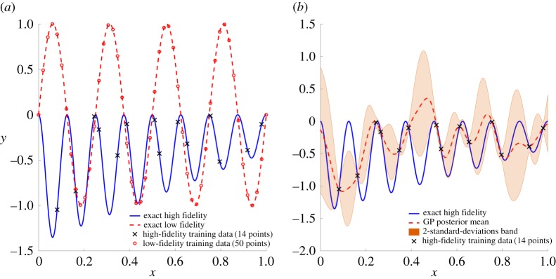
Let us start by considering a deceptively simple example involving two levels of fidelity in one input dimension. The low-fidelity model fl is simply chosen to be a sinusoidal wave with four periods, whereas the high-fidelity model fh is obtained through a transformation of the low-fidelity expression involving a non-uniform scaling and a quadratic nonlinearity, i.e.
| 3.1 |
and
| 3.2 |
Now, assume that we have access only to a finite number of noiseless observations of fl, supplemented by a small number of noiseless observations of fh. In particular, the training sets and are created by randomly sampling the low- and high-fidelity functions at n1=50 and n2=14 points, respectively, making sure that . Figure 1a provides a plot of the low- and high-fidelity functions, along with the points available for training the multi-fidelity GP models.
Figure 1.
A pedagogical example: (a) exact low- and high-fidelity functions (see equations (3.1) and (3.2)), along with the observations used for training the multi-fidelity GP models. (b) Exact solution versus a single-fidelity GP regression trained on the 14 high-fidelity observations. (Online version in colour.)
Using this dataset, our goal now is to reconstruct the high-fidelity signal as accurately as possible. A first intuitive approach would be to train a standard, single-fidelity GP regression using the high-fidelity training points. As summarized in figure 1, this approach cannot provide a reasonable reconstruction of fh as the training data are too scarce to resolve the variability in the underlying signal. Here we must note that this result could improve if one had carefully chosen the GP covariance function. For this specific case, an additive combination of a linear and a periodic kernel would have led to a more expressive GP prior. However, here we focus on a more general approach, hence we deem that further elaborating on manual kernel design is out of the scope of this work.
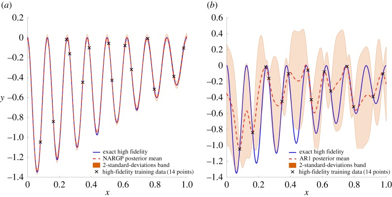
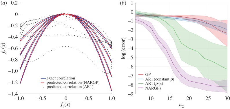
Next, we present the result obtained using the proposed NARGP multi-fidelity algorithm trained on exactly the same high-fidelity data, supplemented with a set of low-fidelity observations, as shown in figure 1a. Evidently, as presented in figure 2a, the NARGP posterior distribution is able to provide an accurate reconstruction of the high-fidelity signal and provide sensible predictive uncertainty estimates as quantified by the 2-standard-deviations band. Remarkably, the NARGP algorithm is able to correctly predict the true underlying signal even at regions where no high-fidelity data are available and also the low-fidelity model is erroneously providing the opposite trend (e.g. for 0.25<x<0.35). This is possible owing to the structure in the NARGP prior (see equation (2.12)) that enables learning the nonlinear and space-dependent cross-correlation between the low- and high-fidelity data, as shown in figure 3a. This is a key feature in constructing resilient multi-fidelity modelling algorithms, as it provides a mechanism to safeguard against wrong trends in the low-fidelity data, while still being able to distil useful information from them. In contrast, the classical AR1 scheme lacks the flexibility needed to capture such complex cross-correlations, and therefore it is not able to use the low-fidelity data. As seen in figure 2b this results in a fit that fails to recover the exact solution, and is qualitatively similar to the single-fidelity GP regression of figure 1b, albeit with less confident uncertainty estimates. In general, these estimates offer a natural quantification of model inadequacy, and constitute one of the most appealing arguments in favour of using GPs over other non-Bayesian approaches (e.g. neural networks, support vector machines).
Figure 2.
A pedagogical example: (a) exact solution versus the NARGP posterior mean and 2 standard deviations for the given multi-fidelity training set. (b) Exact solution versus the AR1 posterior mean and 2 standard deviations for the same multi-fidelity training set. (Online version in colour.)
Figure 3.
A pedagogical example: (a) cross-correlation structure between the exact low- and high-fidelity signals versus the cross-correlation learnt by the NARGP and AR1 schemes trained on the given multi-fidelity dataset. (b) error between the exact high-fidelity signal and the computed posterior mean of the GP, AR1 (constant and input-dependent ρ) and NARGP models, as the number of high-fidelity training points is increased. Shaded regions represent 1 standard deviation from the mean. (Online version in colour.)
In order to asses the sensitivity of our results on the number of training points used, we have performed a series of experiments by fixing the number of low-fidelity training points to n1=50, and increasing the number of high-fidelity points n2 from six to 30 in increments of 2. In all cases, we performed 100 independent repetitions, for each of which we chose the training points at random in the interval x∈[0,1]. Figure 3b shows the computed error between the predicted and exact high-fidelity signal. Evidently, the NARGP multi-fidelity algorithm is able to learn the exact solution with reasonable accuracy using only a minimal number of high-fidelity training points. This significantly outperforms the AR1 scheme, as the latter is unable to leverage the low-fidelity data, and yields a prediction similar to a single-fidelity GP approach. For completeness, we also append the results obtained using the AR1 scheme with a space-dependent cross-correlation factor ρ(x). This case can be viewed as the non-parametric generalization of the scheme proposed by Le Gratiet [14] that considered ρ(x) to assume a given parametric form.
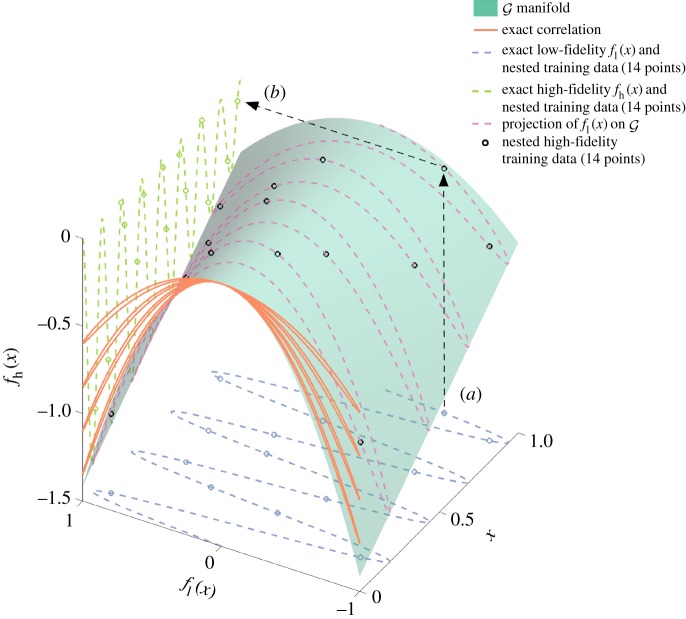
Figure 4 elucidates the key features of the NARGP algorithm that allow for capturing complex nonlinear, non-functional and space-dependent cross-correlations. In particular, note how the low-fidelity model is projected onto the nonlinear latent manifold that is inferred using the deep non-parametric representation of equation (2.11). The manifold is able to correctly capture the cross-correlation structure imposed by the quadratic nonlinearity and the non-uniform scaling in equation (3.2). This effectively ‘disentangles’ the complex functional relation between the low- and high-fidelity data, and is able to recover the target high-fidelity function fh(x) by discovering a smooth mapping from the manifold to the high-fidelity data.
Figure 4.
A pedagogical example: the NARGP algorithm can capture complex nonlinear, non-functional and space-dependent cross-correlations by inferring the nonlinear latent manifold that governs the functional relation between the inputs x and the outputs of the low- and high-fidelity models fl(x) and fh(x), respectively. (a) The low-fidelity model is projected onto the nonlinear latent manifold that is inferred using the deep non-parametric representation of equation (2.11). (b) The high-fidelity function fh(x) is recovered by a smooth mapping from the manifold to the high-fidelity data. (Online version in colour.)
(b). Multi-fidelity approximation of the Branin function
Next, we consider an example with three levels of fidelity in two input dimensions. The highest fidelity data are generated via sampling the non-stationary Branin function [2,20], whereas the medium- and low-fidelity data are obtained through expressions that involve complex transformations of the Branin function, including non-uniform scalings, shifts in phase and amplitude, as well as nonlinearities. The approximation of the Branin function is a popular benchmark problem for surrogate-based modelling and optimization [2,20], and our goal here is to provide a simple yet non-trivial set-up that can be used as a benchmark for future development of multi-fidelity modelling algorithms. In particular, consider the following three functions, indexed by increasing level of fidelity:
| 3.3 |
| 3.4 |
| 3.5 |
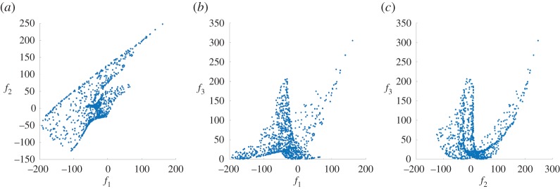
The two-dimensional surfaces corresponding to these expressions are illustrated in figure 5. These surfaces exhibit complex nonlinear spatial cross-correlations as depicted in figure 6 for 1000 randomly sampled points in x∈[−5,10]×[0,15].
Figure 5.
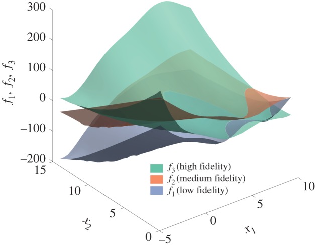
Multi-fidelity approximation of the Branin function: illustration of the exact high-, medium- and low-fidelity response surfaces f1,f2 and f3, respectively. (Online version in colour.)
Figure 6.
Multi-fidelity approximation of the Branin function: (a) spatial cross-correlations between the exact low- and medium-fidelity response surfaces f1 and f2, respectively. (b) Spatial cross-correlations between the exact low- and high-fidelity response surfaces f1 and f3, respectively. (c) Spatial cross-correlations between the exact medium- and high-fidelity response surfaces f2 and f3, respectively. (Online version in colour.)
Given a set of noiseless multi-fidelity observations of f1,f2 and f3, our goal now is to train a multi-fidelity surrogate that can approximate the highest fidelity surface f3. In particular, we consider a nested experimental design consisting of n1=80 low-fidelity, n2=40 medium-fidelity and n3=20 high-fidelity observations, randomly chosen in [−5,10]×[0,15].
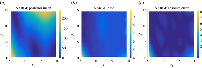
Following the steps outlined in §2c(iii), we train a NARGP multi-fidelity surrogate, and compare the resulting predictions against the classical AR1 multi-fidelity scheme, as well as against standard single-fidelity GP regression trained on the highest fidelity data. Our results, as summarized in figure 7, indicate that the NARGP surrogate was able to accurately reconstruct the highest fidelity response, resulting in a relative error of 0.023 measured in the norm. Moreover, the computed posterior standard deviation provides a good a posteriori error estimate for the maximum absolute deviation from the exact solution, as illustrated in figure 7b,c. Such estimates can be very informative both in terms of assessing the quality of the surrogate model and for actively selecting more training points if the computational budget permits [21,22]. Taken together, these results confirm that the NARGP surrogate was able to successfully infer the complex cross-correlations in the multi-fidelity dataset, and return a sensible predictive posterior distribution.
Figure 7.
Multi-fidelity approximation of the Branin function: (a) NARGP posterior mean, (b) 2 standard deviations and (c) absolute point-wise error with respect to the exact solution f3. (Online version in colour.)
On the other hand, the AR1 multi-fidelity surrogate returns predictions that are about one order of magnitude less accurate, measuring a relative error of 0.112 in the norm. This lower accuracy is also reflected by the higher uncertainty estimates quantified by the AR1 posterior standard deviation which is also one order of magnitude higher than the maximum variance returned by the NARGP model. However, in this example, the AR1 scheme was able to return a better prediction than the single-fidelity GP regression, which yields a relative error of 1.09. This suggests that the AR1 algorithm was indeed able to distil some useful information from the lower fidelity data; however, this was not sufficient for it to provide predictions of comparable accuracy to the NARGP model. In summary, the scatter plot of figure 8 provides a visual illustration of the predictive capabilities of the NARGP, AR1 and GP surrogates in comparison with the exact response f3, evaluated at 1000 randomly chosen test locations.
Figure 8.
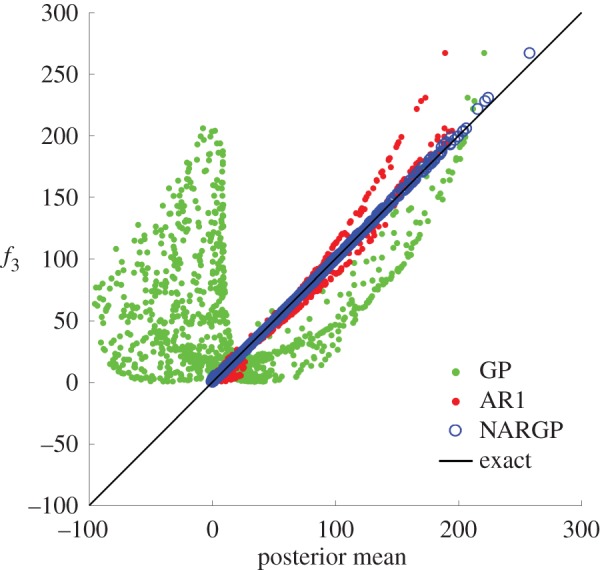
Multi-fidelity approximation of the Branin function: scatter plot of the NARGP, AR1 and GP posterior means versus the exact response f3, evaluated at 1000 randomly chosen test points. (Online version in colour.)
(c). Multi-fidelity modelling of mixed convection based on experimental correlations and numerical simulations
This example aims to showcase the capabilities of the proposed framework in a practical application setting, involving multi-fidelity modelling of mixed convection flows. In a recent study by Babaee et al. [7], the authors employed a multi-fidelity approach based on the recursive AR1 scheme of Le Gratiet et al. [8] to build a data-driven response surface for the Nusselt number for mixed convection flow past a circular cylinder based on experimental correlations and numerical simulations. A schematic of the problem set-up, along with representative snapshots of the temperature solution obtained through high-fidelity direct numerical simulations, is depicted in figure 9a–d. The Nusselt number (Nu) is a non-dimensional quantity defined by the ratio of convective to conductive heat transfer normal to a boundary where heat transfer takes place [7]. In general, mixed convection occurs when natural convection and forced convection mechanisms act together to transfer heat. In such situations, the Nusselt number is a function of the non-dimensional Reynolds (Re) and Richardson (Ri) numbers, as well as the angle ϕ between the forced and natural convection directions [7]. Although the cases of aiding convection (ϕ=0°) and opposing convection (ϕ=180°) have been widely studied and accurate experimental correlations for relating the Nusselt number as a function of (Re,Ri) exist, the regimes resulting from intermediate values of 0<ϕ<180 are relatively underexplored [7].
Figure 9.
Multi-fidelity modelling of mixed convection: (a) sketch of mixed convection of flow over a cylinder. (b,c,d) Representative temperature fields obtained through high-fidelity Navier–Stokes simulations for aiding (ϕ=14.8°), cross (ϕ=97.7°) and opposing (ϕ=152.1°) flows, respectively. (Adapted with permission from Babaee et al. [7].) (Online version in colour.)
In [7], the authors employed the AR1 multi-fidelity scheme to synergistically combine available low-fidelity experimental correlations with a relatively small number of high-fidelity direct numerical Navier–Stokes simulations of mixed convection flow over a cylinder, in order to construct a stochastic response surface for Nu=f(Re,Ri,ϕ) that significantly improves the empirical correlations used so far in mixed convection modelling. It was shown that, although the empirical low-fidelity expressions are relatively accurate for cross-flows with aiding convection (i.e. small Richardson numbers and ϕ<90°), they become increasingly more inaccurate for opposing flows (ϕ<90°) and Ri≃1. Using the AR1 model to perform multi-fidelity information fusion, the authors concluded that, in the latter regime of the input space, low-fidelity correlations are not informative and high-fidelity simulations are needed to accurately capture the nonlinear map Nu=f(Re,Ri,ϕ). We believe that this behaviour is probably the result of the limited expressivity of the AR1 scheme employed in [7], in which a constant cross-correlation parameter ρ was not sufficient to fully capture the correlation structure between the low- and high-fidelity data. This motivates the use of the proposed NARGP algorithm in the hope that it can accurately learn the space-dependent nonlinear cross-correlations between the low- and high-fidelity data, and return a more accurate predictive distribution.
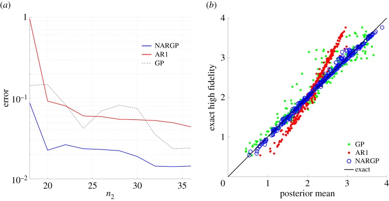
Here, we test the performance of NARGP using the same multi-fidelity dataset employed by Babaee et al. [7]. The dataset comprises 1100 evaluations of the low-fidelity experimental correlations for mixed convection put forth by Hatton et al. [23], and 300 high-fidelity direct numerical simulations of the Navier–Stokes equations past a circular cylinder, as reported in [7]. This nested set of low- and high-fidelity data is created by sampling the input space defined by Re∈[0,100], Ri∈[0,1] and ϕ∈[0,180] using a space-filling Latin hypercube strategy [2]. Following the workflow presented in §2c(iii), we have trained NARGP, AR1 and GP surrogates on a selection of different training sets, constructed by randomly selecting a subset of low-fidelity and high-fidelity training points, where we fix n1=200 and increase n2 from 18 to 36 in increments of 2. To asses the accuracy of each surrogate, we have validated their predictions against the remaining high-fidelity observations that were not used for training. Figure 10a summarizes the results of this experiment by depicting the relative error between the validation data and the posterior mean predictions of each surrogate as the number of high-fidelity training data are increased. Evidently, the ability of the NARGP model to learn the space-dependent cross-correlations between the low- and high-fidelity data yields consistently more accurate predictions for all cases. Moreover, the NARGP model is able to reach accuracy levels that are the same as or better than the AR1 scheme, but with a considerably smaller set of high-fidelity training data. This is attributed both to being more flexible in capturing complex interdependencies in the data as well as to having a very compact parametrization that can be meaningfully trained in data-scarce scenarios. Finally, the scatter plot of figure 10b provides a visual assessment of the accuracy of each surrogate model when trained on n1=200 low- and n2=20 high-fidelity observations, respectively.
Figure 10.
Multi-fidelity modelling of mixed convection: (a) error between the high-fidelity validation data and the computed posterior mean of the NARGP, AR1 and GP models, as the number of high-fidelity training points is increased. (b) Scatter plot of the NARGP, AR1 and GP posterior means versus the high-fidelity validation data, for a training case with n1=200 low- and n2=20 high-fidelity observations. (Online version in colour.)
4. Conclusion
We have presented a novel framework for multi-fidelity modelling using GPs and nonlinear autoregressive schemes. The proposed methodology can be viewed as a fundamental generalization of the classical AR1 scheme put forth by Kennedy & O'Hagan [6], enabling us to learn complex nonlinear and space-dependent cross-correlations in multi-fidelity datasets. We demonstrated the performance of this new class of learning algorithms through a series of benchmark problems involving both synthetic and real datasets. In all cases, the method was able to distill useful information from complex nonlinearly correlated data and outperformed the classical AR1 scheme in terms of predictive accuracy even with less training data. Being able to safeguard our computations against low-fidelity models that may provide wrong trends—a scenario that is quite likely in realistic modelling situations—our nonlinear scheme naturally allows for more flexible and data-efficient multi-fidelity information fusion. Finally, as the difference in computational cost and algorithmic complexity of training the AR1 and NARGP algorithms is negligible, we believe the latter can serve as a drop-in replacement that greatly enhances the capabilities of probabilistic multi-fidelity models.
A drawback of this work stems from the fact that we limited ourselves to cases with noiseless data. Although this is a realistic assumption for all cases considered here—and also in the general context of multi-fidelity modelling of computer codes—this choice rules out many scenarios where noise in the training data plays an important role (e.g. when distilling information from experimental measurements). Here we chose not to address this issue primarily because our aim was to provide a clear presentation of the main ideas behind the proposed framework. However, our methods can be extended to handle noisy or missing data by leveraging the recent work of Damianou & Lawrence [24] on semi-described and semi-supervised learning. In fact, the recursive nature of the proposed algorithm results in independent GP regression problems at each fidelity level, and allows for the straightforward application of any GP model variant (e.g. heteroscedastic GPs for dealing with correlated noise [25], stochastic variational inference GPs for dealing with big data [16], warped GPs for dealing with non-stationary and discontinuous data [26]).
Acknowledgements
The authors also thank Dr Hessam Babaee for sharing the multi-fidelity dataset for the mixed convection flow example.
Data accessibility
The code and datasets supporting this article are available at https://github.com/paraklas/NARGP.
Authors' contributions
P.P., M.R. and A.D. conceived the methods, P.P. implemented the methods, designed and performed the numerical experiments and drafted the manuscript; N.D.L. and G.E.K. supported this study and revised the final manuscript. All authors gave final approval for publication.
Competing interests
We declare we have no competing interests.
Funding
P.P., M.R. and G.E.K. acknowledge support by DARPA EQUiPS grant no. N66001-15-2-4055.
References
- 1.Peherstorfer B, Willcox K, Gunzburger M. 2016. Survey of multifidelity methods in uncertainty propagation, inference, and optimization. Technical Report TR-16-1. Aerospace Computational Design Laboratory, Department of Aeronautics and Astronautics, Massachusetts Institute of Technology, Cambridge, MA, USA.
- 2.Forrester A, Sobester A, Keane A. 2008. Engineering design via surrogate modelling: a practical guide. Chichester, UK: John Wiley & Sons. [Google Scholar]
- 3.Perdikaris P, Karniadakis GE. 2016. Model inversion via multi-fidelity Bayesian optimization: a new paradigm for parameter estimation in haemodynamics, and beyond. J. R. Soc. Interface 13, 20151107 (doi:10.1098/rsif.2015.1107) [DOI] [PMC free article] [PubMed] [Google Scholar]
- 4.Perdikaris P, Venturi D, Karniadakis GE. 2016. Multifidelity information fusion algorithms for high-dimensional systems and massive data sets. SIAM J. Sci. Comput. 38, B521–B538. (doi:10.1137/15M1055164) [Google Scholar]
- 5.Williams CK, Rasmussen CE. 2006. Gaussian processes for machine learning, vol. 2 Cambridge, MA: MIT Press. [Google Scholar]
- 6.Kennedy MC, O'Hagan A. 2000. Predicting the output from a complex computer code when fast approximations are available. Biometrika 87, 1–13. (doi:10.1093/biomet/87.1.1) [Google Scholar]
- 7.Babaee H, Perdikaris P, Chryssostomidis C, Karniadakis G. 2016. Multi-fidelity modeling of mixed convection based on experimental correlations and numerical simulations. J. Fluid Mech. 809, 895–917. (doi:10.1017/jfm.2016.718) [Google Scholar]
- 8.Le Gratiet L, Garnier J. 2014. Recursive co-kriging model for design of computer experiments with multiple levels of fidelity. Int. J. Uncertainty Quant. 4, 365–386. (doi:10.1615/Int.J.UncertaintyQuantification.2014006914) [Google Scholar]
- 9.O'Hagan A. 1998. A Markov property for covariance structures. Stat. Res. Rep. 98, 13. [Google Scholar]
- 10.Damianou AC, Lawrence ND. 2013. Deep Gaussian processes. In Proc. 16th Int. Conf. on Artificial Intelligence and Statistics (AISTATS), Scottsdale, AZ, 29 April–1 May 2013, pp. 207–215.
- 11.Damianou A. 2015. Deep Gaussian processes and variational propagation of uncertainty. PhD thesis, University of Sheffield, Sheffield, UK.
- 12.Mattos CLC, Dai Z, Damianou A, Forth J, Barreto GA, Lawrence ND.2015. Recurrent Gaussian processes. (http://arxiv.org/abs/1511.06644. )
- 13.Bui TD, Hernández-Lobato JM, Li Y, Hernández-Lobato D, Turner RE.2015. Training deep Gaussian processes using stochastic expectation propagation and probabilistic backpropagation. (http://arxiv.org/abs/1511.03405. )
- 14.Le Gratiet L. 2013. Multi-fidelity Gaussian process regression for computer experiments. Thesis, Université Paris-Diderot - Paris VII, France.
- 15.Snelson E, Ghahramani Z. 2005. Sparse Gaussian processes using pseudo-inputs. In Proc. of the 18th Int. Conf. on Neural Information Processing Systems (NIPS'05), Vancouver, British Columbia, Canada, 5–8 December 2005, pp. 1257–1264. Cambridge, MA: MIT Press.
- 16.Hensman J, Fusi N, Lawrence ND.2013. Gaussian processes for big data. (http://arxiv.org/abs/1309.6835. )
- 17.Liu DC, Nocedal J. 1989. On the limited memory BFGS method for large scale optimization. Math. Program. 45, 503–528. (doi:10.1007/BF01589116) [Google Scholar]
- 18.Girard A, Rasmussen CE, Quinonero-Candela J, Murray-Smith R. 2003. Gaussian process priors with uncertain inputs. Application to multiple-step ahead time series forecasting. In Advances in neural information processing systems 15 (eds S Becker, S Thrun, K Obermayer), pp. 545–552. Cambridge, MA: MIT Press. See http://papers.nips.cc/paper/2313-gaussian-process-priors-with-uncertain-inputs-application-to-multiple-step-ahead-time-series-forecasting.pdf.
- 19.GPy. 2002. GPy: A Gaussian process framework in python. See http://github.com/SheffieldML/GPy.
- 20.Surjanovic S, Bingham D. Virtual library of simulation experiments. Test functions and datasets. See http://www.sfu.ca/ssurjano.
- 21.MacKay DJ. 1992. Information-based objective functions for active data selection. Neural Comput. 4, 590–604. (doi:10.1162/neco.1992.4.4.590) [Google Scholar]
- 22.Cohn DA, Ghahramani Z, Jordan MI. 1996. Active learning with statistical models. J. Artif. Intell. Res. 4, 129–145. [Google Scholar]
- 23.Hatton H, James A, Swire D. 1970. Combined forced and natural convection with low-speed air flow over horizontal cylinders. J. Fluid Mech. 42, 17–31. (doi:10.1017/S0022112070001040) [Google Scholar]
- 24.Damianou A, Lawrence ND. 2015. Semi-described and semi-supervised learning with Gaussian processes. (http://arxiv.org/abs/1509.01168. )
- 25.Titsias MK, Lázaro-gredilla M. 2011. Variational heteroscedastic Gaussian process regression. In Proc. of the 28th Int. Conf. on Machine Learning (ICML-11), Bellevue, WA, 28 June–2 July 2011, pp. 841–848.
- 26.Snelson E, Rasmussen CE, Ghahramani Z. 2004. Warped Gaussian processes. Adv. Neural Inf. Process. Syst. 16, 337–344. See http://machinelearning.wustl.edu/mlpapers/paper_files/ICML2011Lazaro-Gredilla_456.pdf. [Google Scholar]
Associated Data
This section collects any data citations, data availability statements, or supplementary materials included in this article.
Data Availability Statement
The code and datasets supporting this article are available at https://github.com/paraklas/NARGP.


