Forecasting the Spread of Mosquito-Borne Disease using Publicly Accessible Data: A Case Study in Chikungunya

Abstract

Mosquito-borne diseases account for multiple public health challenges in our modern world. The international health community has seen a number of mosquito-borne diseases come to the forefront in recent years, including West Nile virus, Chikungunya virus, and currently, Zika virus. Predicting the spread of mosquito-borne disease can aid early decision support for when and how to employ public health interventions within a community; however, accurate and fast predictions, months into the future, are difficult to achieve in urgent scenarios, particularly when little information is known about infection rates. New sources of information including social media have been proposed to accelerate the development of predictive models of disease progression. In this research, we adapted a previously described model for the spread of mosquito-borne disease using open intelligence sources. The novel implementation of a mixed-model for mosquito-borne disease was capable of being executed in minimal runtime. The results indicate that this model yields fast and relevant results with acceptable margins of error.

Introduction

In August 2014, in response to the rising threat of the Chikungunya virus in 47 Pan-American countries, the United States Defense Advanced Research Projects Agency (DARPA) announced its “Forecasting Chikungunya” Challenge, supported by Innocentive.com¹. The goal of this challenge was to gather researchers, analysts, and interested parties to investigate and predict how the Chikungunya virus (CHIKV) would impact populations in 55 countries with relatively untested immunities, such as the United States². Strategies for preventing the spread of Chikungunya on an individual level typically include avoiding travel to emergent areas, wearing clothing that covers extremities and exposed skin, using mosquito nets for beds, and of course, the usage of repellant³. Public health officials can encourage prevention as well by distributing mosquito nets, spraying densely mosquito-populated areas, and while notifying the public at large of methods for prevention. However, with CHIKV threatening the estimated 950 million individuals currently living in Pan-American countries, it is helpful to determine where the virus may hit hardest in tandem with, if not before, implementation of prevention strategies. There are a number of epidemiological strategies for modeling the spread of mosquito-borne diseases such as dengue fever⁴, malaria⁵, and yellow fever⁶. In 2012, Ruiz-Moreno et al. introduced a combined climate and epidemiological model for predicting the spread of Chikungunya virus in the United States via the Aedes mosquito, finding that climate-based changes could be used to classify regions of the US according to epidemic risk⁷. In this model, Ruiz-Moreno et al. incorporated parameters for mosquito and human population density, temperature, and initial infection rates to forecast the potential peak of CHIKV with enough accuracy to recommend potential areas for targeted public health interventions, should the need arise.

To address DARPA’s call for methods to forecast the spread of CHIKV, we have implemented and modified Ruiz- Moreno’s model to extend it for use in any country or region, but specifically implemented it for Pan-American countries. The model was implemented for the months of September 2014 to February 2015, as per DARPA’s solicitation. This model takes as input total country population (N), land area (km²), mosquito population (M), temperature (C) and number of infected individuals (I). The population and area variables can easily be computed using available online resources (described further in Methods) and mostly remain constant, so the model largely depends on the current temperature (also easily found online, but frequency of change is according to the user), the mosquito population (estimated) and the number of infected individuals. In the Methods section, we describe how we are able to collect these parameters using publicly available data and calculate or infer other parameters required to run the model. We have implemented the model using the R programming language to discern the rise in infected individuals, per country, on a weekly basis.

Methods

To forecast the number of cases infected with Chikungunya Virus (CHIKV) across the Americas, we modified the model proposed by Ruiz-Moreno et al.⁷. The modified model, which we will informally identify as our SEIRM model, uses ordinary differential equations to simulate the dynamics of mosquito-borne infections in human populations. In particular, the human population is divided into susceptible (S), exposed (E), infected (I), and recovered (R) individuals. The mosquito population is also subdivided into immature eggs, larvae, eggs under diapause, and mature susceptible, exposed and infected. Parameters related to the life-cycle of the Aedes mosquito were taken from the literature, as reported in Ruiz-Moreno et al⁷. All of the data sources described below used for the forecasts are freely available and readily accessible.

Data Sources

The main data sources used included information from news reports gathered via an automated news information system (solely from HealthMap.org), weather data, and population and country size data. The model requires the following initial conditions: 1) the number of susceptible, exposed, infected, and recovered individuals in a given country; 2) the size of the mosquito population. The number of infected cases per country was extracted from HealthMap (www.HealthMap.org), an automated system that monitors information sources on outbreaks⁸. The rationale behind choosing HealthMap is that it provides almost instantaneous reports at a local level, as opposed to more traditional surveillance systems that may be lagging behind in their reports. This information can be filtered by species, disease, dates, and location; the data collected particularly for CHIKV was reported as it happened and not on a regular interval (i.e. a country was only reported to have cases on HealthMap if cases were found that day, week, or month). HealthMap was the main source for CHIKV infection numbers, but it does have some disadvantages. In some cases, HealthMap provides case numbers for entire countries and cities within those countries; the numbers provided for major cities might be contained within the country level estimate. To account for this, only numbers counted for entire countries were considered for this project. A second issue is that in some cases numbers were reported based on data mined from news reports, resulting in inaccurate reports on HealthMap. For example, in an article that may have stated “Experts believe cases could reach up to 100,000 in Chile,” HealthMap may report 100,000 cases for Chile when the actual number of cases would be much lower. This is an issue that seems to have been resolved on the website but was present in the early stages of the project. Some countries never had reported numbers of cases, or in the case of the Caribbean Islands, numbers were reported in groups (i.e. “St. Bart’s, St. Vincent, and St. Kitts collectively have X amount of cases.”) Finally, due to inconsistency of CHIKV reporting, there could be a long absence of reported cases for any given country and then a week where new numbers were reported everyday; the question remained which number to be used. As a result of these issues, we adopted the following guidelines for collecting CHIKV infection numbers from HealthMap:

• 1. For a given month, if a country reported infected cases on CHIKV, the most recent number of cases was recorded for our forecast (even if this number was not the highest possible).
• 2. If there was a large deviation from previous numbers (for example, one case reported in August and then 50,000 cases reported in September), the articles were manually investigated for their veracity – the most recent number with the most likely cases reported was recorded for use in the forecast.
• 3. Only numbers reported for countries were used; numbers for individual cities contained within eligible Pan-American Health Organization (PAHO) countries were ignored.
• 4. If a country had no cases reported for that time interval, a Google News search for the country’s name and chikungunya (i.e. “Anguilla chikungunya”) was performed to validate that no cases had been reported. If an article was found where some cases had been reported, it was individually evaluated for reliability and if it was deemed a reputable source, that number was recorded. If this scenario occurred, the source of the number recorded was also recorded.
• 5. If no change had been reported from month to month for a country via HealthMap and no reputable new source was found via a Google News search, the initial number of infected was not changed.
• 6. For each country at each forecast, we have recorded whether the number of infected cases came from HealthMap or a news article found via Google News search.

The CHIKV numbers were recorded as described above via HealthMap and other sources were used for each country as the initial number of Infected. To estimate the other initial values (Susceptible, Exposed, Recovered), the

total population was found for each country via Google search (i.e. “Anguilla population”) and recorded using the following approach. Given a list of C = {c₁, c₂, …, c_N) countries provided, a Google search for each country in C was performed using the search term “c, population” where c_i represents the current country in C. This search was done manually as less than 100 countries were being studied and to use an API would require more time and work than just searching manually. For country population, Google provides not only a list of search results in the form of hyperlinks, but also a “definitive” population based off the last major formal census of the region as the top result. This is the number that was used to determine the total country population – the definitive population stored by Google’s “Map Data” resource. The values for remaining compartmental populations of a country (Susceptible, Exposed, and Recovered) were estimated using the following simple equations (chosen arbitrarily to reflect reasonable and conservative estimates):

Given the Country population (P) and Infected Population (I):

Recovered (R) = I * 0.75

Susceptible (S) = (P – I – R)*0.9

Exposed (E) = (P – I – R)*0.01

Initially, the Exposed population was set to (P-I-R)*0.1 to ensure that S+E+I+R = P. However, in our model this resulted in a very large number of persons becoming infected and was felt to inaccurately describe a realistic scenario of exposed persons. As such, in October forecasts and further, a new Exposed equation was adopted and each country was held to the condition that S+E+I+R < P.

To estimate the size of the mosquito populations at a per-country level, we used mosquito density data reported by Eiras and Resende for Brazilian municipalities⁹, and the surface area of each country. Although the estimates are necessarily only approximations, we found a change in predictive power over simply using a fixed number of mosquitos for each country.

The average monthly temperature (AMT) in Celsius was collected for each country for every month from 2001 to 2010. Latitude, longitude, and temperature data was downloaded from the following website provided by The Centre of Climatic Research, University of Delaware¹⁰. The Google maps API was used to convert the latitude and longitude information to its respective country name. Temperature data for a country was calculated as the average of temperature readings from all the points in that country. For each month from 2001 to 2010, the AMT was averaged to get a single value for input into the model. As such, for every forecast, the input parameters for weather changed according to the average of all AMTs for that country in that month from 2001 to 2010.

Model Implementation:

The aforementioned modified Ruiz-Moreno model was implemented in R using the deSolve() library and an array of inputs and parameters described below. Equations that have been modified from the Ruiz-Moreno manuscript are highlighted in bold and described in a comment; many of these modifications are very small. All involve removing a density-dependent parameter specified in the original paper that was defined only for certain US cities (Miami, Atlanta, and New York) and these parameters could not be effectively estimated for duplication in our model. Very brief pseudocode of the model can be found below. The code for the model can be found at https://github.com/katecooperOMA/Chikungunya.

/***Begin model***/

1  Load library deSolve and  other requirements

2  /***Load inputs by user***/

3  initials = {

4     country = user input

5     S = user input   #Susceptible

6     E = user input   #Exposed

7     I = user input   #Infected

8     R = user input   #Recovered

9     G = user input   #Mosquito population by country size

10    temp = user input   #Average AMT for country during current month

11  }

12  /***Load Hard Parameters by Ruiz-Moreno***/

13   parameters = { Adult mosquito population, symptomatic/asympomatic ratio, etc. }

14

15   /**Load Soft parameters by Ruiz-Moreno #See [7]for full definitions***/

16   parameters = {mosquito egg mortality, larval mortality, incubation period, etc

17

18   population = S+E+I+R}

19  dT = sequence 1 to 4 by 1/7     #define the time interval desired

20    SEIRM_function = {

21    define changes in mosquito populations (adult, larval), compartmental populations)

22    population = S+E+I+R

23  der<-c(dS,dE,dI,dR,dG,dD,dL,dAs,dAe,dAi) #der is a function of deSolve library

24   }

25

26   simulation<-as.data.frame(lsoda(initials,dT, SEIRM_function,parameters))

27   output results

For each forecast, the inputs (S,E, I, R, G, country name, and temperature) were collected and ran using a small Perl wrapper that iteratively ran each command in a designated folder where outputs and error logs, if any, were collected. The model gives S, E, I, and R predictions for 21 weeks after the initial values but only the Infected numbers are recorded. Because the country temperature input changed from month to month, the model was run for every month remaining in the forecast. For example, for the December 1 forecast, the model was run three times: once for December, once for January, and once for February. The output of Decembers forecast, then, became the input for January’s forecast, i.e., if the number of infected cases for the last week of December was predicted to be 30, then 30 was used as the initial value of Infected for the January iteration of the December forecast. Similarly, the last week of the January forecast then became the initial value for the February model iteration. This was structured according to the DARPA Forecasting Chikungunya Challenge guidelines¹¹.

A number of parameters used in our model were held steady at every iteration; these included: the adult mosquito population, the number of eggs per mosquito per day, the rate of symptomatic to asymptomatic individuals, the biting rate of the mosquito, the infective period, the probability of both human-to-mosquito and mosquito-to-human transmission, the density dependent factor for reproduction and density function, and the natural and disease- induced mortality rates. The numbers are estimates and were taken from Ruiz-Moreno et al.¹ and after discussion, it was determined that none of these parameters had enough evidence to warrant their change in our model in its early stages. Other constant parameters included were country population and area/size.

Saint Martin and Sint Maarten were counted as two separate countries.

Results

Real-world Performance. The ability to effectively display the results of simulations is particularly important in this domain, where several different scenarios might have to be explored and interpreted by professionals with diverse backgrounds and expertise. Our model generates an easily interpretable time-dependent chart, illustrating the number of predicted susceptible, infected, and recovered cases over a given time range.

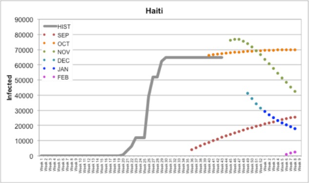
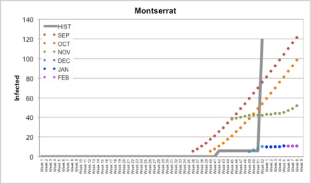
In Figure 1, we documented our forecasts for all months (September, October, November, December, January, and February) compared to Historical PAHO data in Haiti. For example, our September forecast for Haiti predicted a slow rise to around ~30,000 infected cases reported by February (Figure 1); by the time the October forecast came due, HealthMap had reported several cases in Haiti and future predictions reflected this update. With a population around 103 million, the number of cases in Haiti was predicted to represent around 90,000 or 0.87% of the population. This prediction model also applies well to smaller countries. A similar data plot is shown below for Montserrat (Figure 2), which has a population of around 5,900 individuals. Our initial predictions for September and October predicted a rise to approximately 100 or 120 infected individuals by February; in the final week of December, Montserrat reported an increase in cases from 6 (first reported in Week 42) to 119 (reported in Week 52). However, with few to no cases reported by HealthMap in December or January and a change in temperature, our December, January, and February forecasts assumed a low initial Infected value and a slow climb in the number of cases. Still, at 119 cases, this represents about 2% of Montserrat’s total population.

Figure 1.

Our forecasts for Haiti compared to Historical PAHO data (HIST)

Figure 2.

Our forecasts for Montserrat compared to Historical PAHO data (HIST)

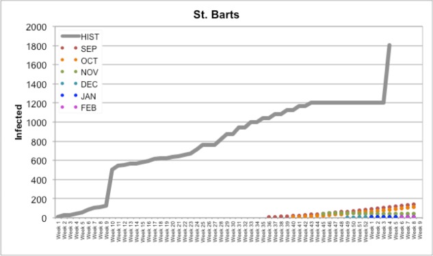
St. Bart’s (Figure 3) is an example of a case where nothing was being reported specifically for the country in the news or on HealthMap itself; occasionally it would be included in a count for a group of countries, but being a small island with a small population, this country did not manifest itself it the news often. As a result, our forecasts predicted a slow rise in the number of cases (compared to the actual number of cases reported); when these predictions did not reflect the HealthMap/news data released in the next month, the slow rise in cases was simply pushed back by the model to the next month.

Figure 3.

Our forecasts for St. Bart’s compared to Historical PAHO data (HIST)

For countries where the mosquito population is not regularly be exposed to CHIKV, such as the United States or Canada, our initial forecasts predicted far too many cases because numbers for exposure and mosquito populations were not modified (Figure 4). However, once the temperatures in these countries dropped, our predictions became (slightly) more accurate

Figure 4.

(Left) All forecasts for the United States and (Right) the December, January, and February forecasts for the United States

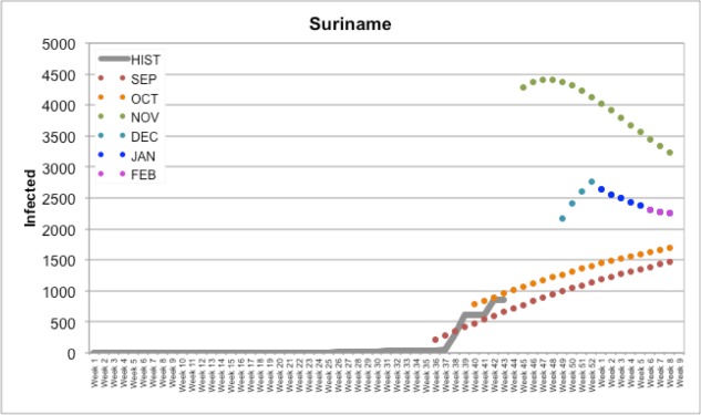
Suriname (shown in Figure 5) is an example of a country where we are not yet quite sure how well our predictions have come out; as of the time of this manuscript they had not reported their CHIKV cases since Week 44. All indicators suggest that while we had a few differences in the severity of infectiousness trend, this prediction may be one that is more accurate than others. Further, we can also potentially display the number of cases on a geographic map over time, a type of representation that is particularly useful to track the spread of the disease and the effects of containment measures in specific areas.

Figure 5.

Our forecasts for Suriname compared to Historical PAHO data (HIST)

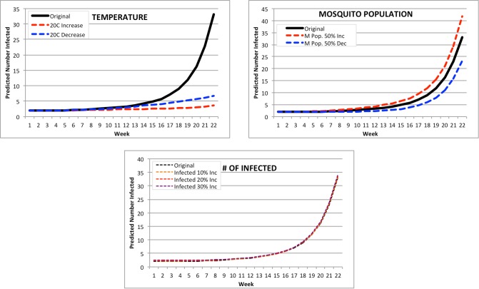
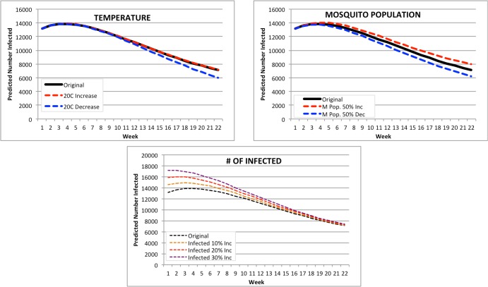
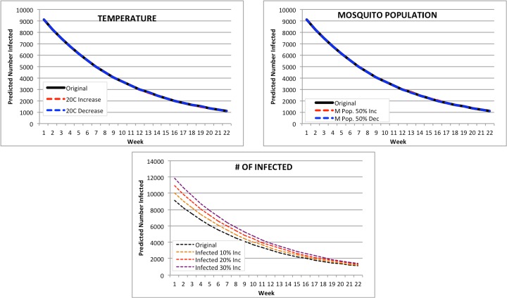
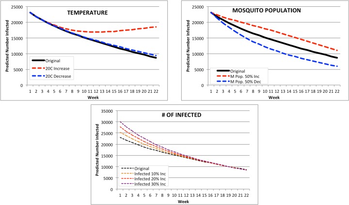
Sensitivity Analysis. It is difficult to perform accurate sensitivity or uncertainty analysis on our model due to incomplete and inconsistent PAHO reporting. However, we have completed some tests to investigate how much our forecast would deviate by modifying temperature, mosquito population, and number of infected for the most populous country (United States at 313 million), the least populous country (Saba at 1,824), the median country for population (Guadeloupe at 17 million) and the average country for population (Chile at 405,739). We ran our forecast for 22 weeks based on our input data for February 2015 for each of these countries, and identified three major areas of modification to investigate: (1) change in the original input temperature (+ or -20C), (2) change in mosquito population (+ or – 50% of the February input mosquito population), and (3) change in the number of infected (increases of 10%, 20%, and 30% of the February input of infected cases). The results of these iterations are below.

Saba: the smallest PAHO country by population (Figure 6). The number of infected for Saba was only distinctly affected by the temperature – it would appear based on the curves for both an 20C increase and decrease in temperature that the ideal temperature for CHIKV spread would be around the current average temperature there, 27.2C. However, the forecast shown assumes this temperature remains the same for the next 20 weeks – this would not be the case in a real world situation. Changes in mosquito population and number of infected have minimal effect on the outcome of the 22 week forecast, with mosquito population having a 22 week range of ~25-45 infected and number of infected forecasts all having a 22-week prediction of ~35 infected.

Figure 6.

Modified Forecasts for Saba. Top left: Forecasts for original Feb. 2015, or with a + or -20C input modification. Top right: Forecasts for original Feb. 2015, or with a + or -50% mosquito population. Bottom: Forecasts for original Feb. 2015, or with a ⩲ 10%, 20%, or 30% population increase.

Chile: the average PAHO country by population (Figure 7). None of the forecasts for Chile were distinctly affected by any change in parameter. A change in temperature resulted in a 22-week prediction range of 5966 infected (20C decrease) to 7158 for a 20C increase, a difference of only 1192. A change in mosquito population resulted in a range of 6222 to 7990 infected for a 50% decrease and a 50% increase respectively. The increase in number of infected resulted in a predicted range of 7208 (10% increase) to 7360 infected (30% increase).

Figure 7.

Modified Forecasts for Chile. Top left: Forecasts for original Feb. 2015, or with a + or -20C input modification. Top right: Forecasts for original Feb. 2015, or with a + or -50% mosquito population. Bottom: Forecasts for original Feb. 2015, or with a + 10%, 20%, or 30% population increase.

Guadalupe: the median PAHO country by population (Figure 8). None of the forecasts for Guadaloupe were distinctly affected by any change in parameter; in fact, two of the modifications (temperature and mosquito population change) had almost no impact on predicted number of infected at all. A change in temperature resulted in a 22-week prediction range of 1,101 infected (20C decrease) to 1,093 for a 20C increase, a difference of only 8. A change in mosquito population resulted in a range of 1,097 to 1,112 infected for a 50% decrease and a 50% increase respectively. The increase in number of infected resulted in a predicted range of 1,203 (10% increase) to 1,402 infected (30% increase).

Figure 8.

Modified Forecasts for Guadaloupe. Top left: Forecasts for original Feb. 2015, or with a + or -20C input modification. Top right: Forecasts for original Feb. 2015, or with a + or -50% mosquito population. Bottom: Forecasts for original Feb. 2015, or with a + 10%, 20%, or 30% population increase.

United States: the largest PAHO country by population (Figure 9). The forecasts for the United States were the most affected by any changes both temperature and mosquito population. A change in temperature resulted in a 22-week prediction range of 9,333 infected (20C decrease) to double that at 18,556 for a 20C increase. However, the original February forecast inputs were very similar in range to the 20C decrease in temperature, suggesting that the 20C increase or decrease signaled a change in mortality for mosquito populations, thus affecting the number of infected. A change in mosquito population resulted in a range of 5,992 to 11,048 infected for a 50% decrease and a 50% increase respectively. The increase in number of infected resulted in a predicted range of 8,574 (10% increase) to 8,470 infected (30% increase).

Figure 9.

Modified Forecasts for the United States. Top left: Forecasts for original Feb. 2015, or with a + or -20C input modification. Top right: Forecasts for original Feb. 2015, or with a + or -50% mosquito population. Bottom: Forecasts for original Feb. 2015, or with a + 10%, 20%, or 30% population increase.

These results suggest that our model is potentially at its best when dealing with populations in the average or median range, but can also perform on very small and very large populations. The biggest changes observed were between the parameter modifications in the United States, the largest PAHO country by population. Compared to the forecasts of Guadaloupe (with a population of 17 million), this suggests that a threshold for integrity of the model as it sits currently may lie somewhere between 17 and 300 million population. All of this, of course, is speculative at best – more rigorous robustness testing with accurate PAHO data would better reveal the strength and predictive power of the model.

Applicability. The SEIR model that was used for our predictions can be easily applied to other mosquito-borne diseases such as Malaria, West Nile, dengue fever, Congo-Crimean hemorrhagic fever, or yellow fever. Depending on the type of disease, parameters related to the infectivity of the agent and to the life cycle of the vector would have to be suitably chosen, but the general structure of the model does not require major changes. This extends to diseases transmitted via other vectors such as ticks to humans and animals alike; the main dependencies of the model lie in initial values, population, temperature, and area of a country or district. Of course, the model can be modified. In fact, related SIR (Susceptible, Infected, Recovered) models have been successfully used in the past to model the spread of dengue fever and other borne infectious diseases [4][5]. This could, then, theoretically be applied to other diseases such as Ebola or measles, with relatively small changes.

Computational Resources. The model does not require specialized hardware, and can run on a desktop computer or laptop. It is implemented in the widely used R language, which is freely available for Windows, Mac OS X, and Linux platforms. A simulation takes approximately 15-30 seconds for all countries on a Late 2013 MacBook Pro with 2.4 GHz Intel processor running OS X 10.9.3.

The model is general in its implementation, and can be easily adapted to accept data sources that are different from the ones that were used for this research. For example, instead of news reports from HealthMap the model could use surveillance data or other sources containing the incidence of new cases. Furthermore, all of the data collection and processing can be scripted and automatically run at certain intervals without user interaction.

Conclusion

Our modified Ruiz-Moreno model is a simple and easily interpretable approach that uses freely available data. The datasets used as input are reliable, ranging from very high confidence (population and country area/size) to moderately reliable (HealthMap data and news reports). The model runs very quickly (under 1 minute) on most laptop computers equipped with the R statistical suite and the essential libraries discussed previously. Additionally, our model is discriminatory – it remains free of extraneous variables and data by depends largely on initial values, temperature, population and land area to determine rates of infection. More variables can be added as they are deemed important by public health authorities. The contribution of this research is a novel implementation of a mixed model for -borne disease that executes in minimal (<5 minute) runtime using only publicly available information.

References

- 1.DARPA Forecasting Chikungunya Challenge [Internet]. 2014 Aug 15 [cited 2016 Mar 3] Available from: https://www.innocentive.com/ar/challenge/9933617?cc=DARPApress.
- 2.Charrel RN, de Lamballerie X, Raoult D. Chikungunya outbreaks-the globalization of vectorborne diseases. New England Journal of Medicine. 2007 Feb 22;356(8) doi: 10.1056/NEJMp078013. [DOI] [PubMed] [Google Scholar]
- 3.Nasci RS, Wirtz RA, Brogdon WG. Protection Against Mosquitos, Ticks, & Other Arthropods [Internet]: Centers for Disease Control and Prevention. 2015 July 10 [last updated 2015 July 10, cited 2016 Mar 3] Available from: http://wwwnc.cdc.gov/travel/yellowbook/2016/the-pre-travel-consultation/protection-against- mosquitoes-ticks-other-arthropods.
- 4.Derouich M, Boutayeb A, Twizell EH. A model of dengue fever; BioMedical Engineering OnLine.; 2003. Feb. 4 pp. [DOI] [PMC free article] [PubMed] [Google Scholar]
- 5.Ngwa GA, Shu WS. A mathematical model for endemic malaria with variable human and mosquito populations. Mathematical and Computer Modelling. 2000 Oct.32(7):747–63. [Google Scholar]
- 6.Dye C. Models for the population dynamics of the yellow fever mosquito, Aedes aegypti. The Journal of Animal Ecology. 1984 Feb.:247–68. [Google Scholar]
- 7.Ruiz-Moreno D, Vargas IS, Olson KE, Harrington LC. Modeling dynamic introduction of chikungunya virus in the United States. PLoS Negl Trop Dis. 2012 Nov.6(11) doi: 10.1371/journal.pntd.0001918. [DOI] [PMC free article] [PubMed] [Google Scholar]
- 8.Brownstein JS, Freifeld CC, Reis BY, Mandl KD. Surveillance Sans Frontieres: Internet-based emerging infectious disease intelligence and the HealthMap project. PLoS Med. 2008 Jul.5(7) doi: 10.1371/journal.pmed.0050151. [DOI] [PMC free article] [PubMed] [Google Scholar]
- 9.Eiras ÁE, Resende MC. Preliminary evaluation of the “Dengue-MI”. technology for Aedes aegyptimonitoring and control. Cadernos de SaÁde PÁblica. 2009;2(5):S45–58. doi: 10.1590/s0102-311x2009001300005. [DOI] [PubMed] [Google Scholar]
- 10.Willmott C. J, Matsuura K. Terrestrial Air Temperature. Monthly and Annual Time Series 1950 – 2010, 2001 http://climate.geog.udel.edu/~climate/html_pages/download.html#P2011rev. [Google Scholar]
- 11.The DARPA Innocentive Chikungunya Challenge guidelines were only available to Challenge solvers during the tenure of the challenge itself and are no longer available on the website. While we do not have permission to publicly post these guidelines, a digital copy of the guidelines can be shared upon request