Predicting Negative Events: Using Post-discharge Data to Detect High-Risk Patients

Abstract

Predicting negative outcomes, such as readmission or death, and detecting high-risk patients are important yet challenging problems in medical informatics. Various models have been proposed to detect high-risk patients; however, the state of the art relies on patient information collected before or at the time of discharge to predict future outcomes. In this paper, we investigate the effect of including data generated post discharge to predict negative outcomes. Specifically, we focus on two types of patients admitted to the Vanderbilt University Medical Center between 2010-2013: i) those with an acute event - 704 hip fractures and ii) those with chronic problems — 5250 congestive heart failure (CHF) patients. We show that the post-discharge model improved the AUC of the LACE index, a standard readmission scoring function, by 20 - 30%. Moreover, the new model resulted in higher AUCs by 15 - 27% for hip fracture and 10 - 12% for CHF compared to standard models.

Introduction

Predicting events associated with negative outcomes, such as readmission or death, post discharge is challenging. Traditionally, negative outcome prediction systems are executed at the time of discharge to identify high-risk patients¹. However, such systems are limited in their applicability because patient status often changes after their discharge and risk prediction models are not amended to incorporate such information. This lack of knowledge can result in risk assessment errors and potential readmission penalties, under Meaningful Use regulation, calculated via a payment adjustment factor².

Care providers, as well as the administrators of healthcare organizations, are keen on determining which patients might experience complications that lead to readmission or death, so that they may allocate additional resources to the patients and intervene before a negative outcome transpires³. Unfortunately, resources are limited and decision makers within health organizations (e.g. physicans and care coordinators) specify a subset high-risk patients who can receive special attention while other high-risk patinets do not have access to such resources^{4, 5}. Accurately identfying, as well as prioritizing, which patients should be assigned assistance is an important informatics problem.

To investigate the effect of post discharge data in predicting negative outcomes, we focus on several core questions. First, what post-discharge information is available for prediciton? Second, how can a post-discharge model be formulated? And, finally, how do different time periods of post-discharge information impact such predictions? In doing so, we examine which post-discharge features are the most important drivers of negative outcome predictions.

We evaluated standard and post-discharge prediction models using three years of data from Vanderbilt University Medical Center’s (VUMC’s) electronic medical record (EMR) system for two phenotypes : 1) an acute condition in the form of a hip fracture and 2) and a chronic progressive disorder in the form of congestive heart failure (CHF). The results demonstrate that:

• Running the prediction at successive post-discharge days, and including post-dischrage clinical information in the prediction model, outperforms state-of-the-art “at discharge” models, such as LACE^{6 7};

• The importance of post-discharge clinical features grows as the prediction horizon for negative events is pushed further into the future; and

• Higher utilitization of clinical resources (e.g. appointments and medications) are correlated with a negative outcome.

Background

The number of proposed risk prediction models has increased dramatically over the last decade. Kansagara and colleagues performed a comprehensive systemic review to evalute the performance of risk prediction models and their suitability for clinical use ¹. To evaluate the performance of the risk model, studies usually compare their models to an established model such as LACE. This is a readmission index that provides a risk score to predict the readmission or death, specifically for CHF patients, using length of stay (L), the acuity of admission (A), comorbidity score (C), and the number of the emergency department visits (E)^{6, 7}.

Several studies have shown that post-discharge data can assist in the prediction of negative events in special circumstances. For instance, certain studies focused on surgical quality assessment at the point of discharge observed that over a quarter of the complications are diagnosed post-discharge^8–10. In another study, it was found that post-discharge data could improve the prediction of the presence, as well as the severity, of spasticity in upper limbs in the year following a stroke¹¹.

While post-discharge data has rarely been used in readmission prediction, Hersh and colleagues performed a systemic review about the post-discharge environment and its relation to readmission after heart failure¹². They reviewed 26 studies published between 1985 and 2011 to evaluate the importance of integrating post-discharge environment in the heart failure readmission model. In the review, only 7 studies included post-discharge data and focused mainly on whether the patient had a primary care provider. They concluded that the socio-economics of the post-discharge enviroment is a key indicator that affects readmission probability. Another factor that has been found to correlate with readmisson is follow-up after discharge. Specifically, patients with a larger number of early followups tend to have a lower likelihood of unplanned readmission, especially for patients with a greater collection of comorbidities¹³-¹⁶.

Methods

In this section, we describe the risk prediction models. First, we describe methods to construct features using data from different post-discharge time windows. Second, we use these features to predict negative events occurring up to a prediction window.

Prediction Model Composition

We represent longitudinal EMR data with an M^NxT matrix, where T is the length of time for extracted EMR data and N is the number of patients in the cohort. Each row in the matrix represents one patient vector denoted by t. For each patient p, we divide the longitudinal medical record vector t into three temporal bins: before admission, during admission, and after discharge. For each model, we define an observation window (OW) that specifies the time from which to extract features. Using combination of features, we predict whether the patients would have a negative outcome within a prediction window (PW), where the window starts at the discharge day and ends at the prediction point (PP).

For the purposes of this investigation, we represent outcomes as a dichotomous variable. A patient has a negative outcome if he/she experiences a negative event (-1) in the prediction window and has a non-negative outcome (+1) otherwise. Figure 1 visualizes model settings in which both patients experience negative outcomes, but only the patient in Figure 1b has a negative outcome in the prediction window.

Figure 1.

Prediction models based on temporal features (a) before and (b) after a negative outcome.

We construct the following prediction models by varying the combination of observation windows and features:

Model 1: LACE: Starting with the most common method in the literature, we build a prediction model using LACE, where E was restricted to the number of the emergency department visits in the past 6 months. LACE assigns points to each variable based on its value, and calculates probabilities by using regression models⁷. Patients with a score greater than 10 are considered to be high risk. We retrieved the features utilized by LACE from the EMR and calculated the risk score, which was fed as a feature into the prediction model. We consider LACE as the baseline for performance comparison.

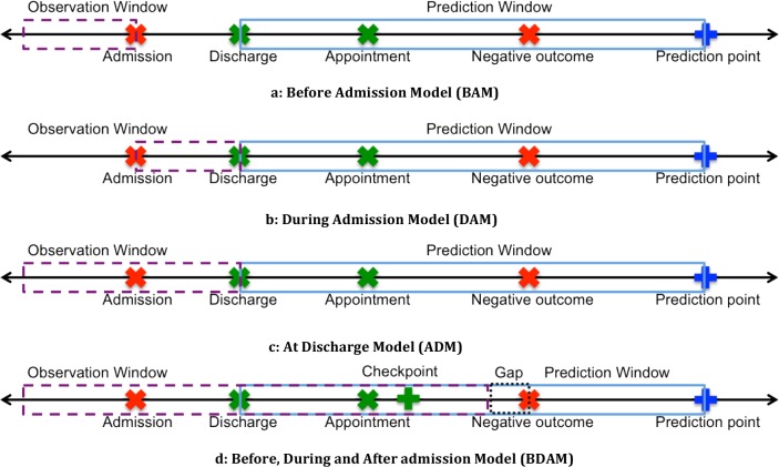
Model 2: Before-Admission Model (BAM): To learn whether prior health status can be applied to forecast the future health status of patients, we use only data from before the admission to predict the outcome. Each patient’s entry is assigned to a pre-admission feature vector denoted by b. The BAM matrix is visualized in Figure 2a.

Figure 2.

Prediction models based on varying temporal features.

Model 3: During-Admission Model (DAM): We investigated whether the data collected about investigated phenotype is sufficient to predict the outcome. The observation window begins at admission and ends at discharge and is visualized in Figure 2b.

Model 4: At-Discharge Model (ADM): This model incorporates data from before and during admission to predict the outcome, and is visualized in Figure 2c.

Model 5: Before, During admission, and After discharge Model (BDAM): The last model incorporates postdischarge data to predict the patient’s outcome, which is visualized in Figure 2d. There are several key parameters to this model: 1) the time window post-discharge to include data, which we refer to as a checkpoint, 2) the length of the prediction window, and 3) ensuring that data prior to negative events does not introduce biased knowledge about an upcoming negative event. Regarding point (3), we remove data from days immediately before the end of the window, which we refer to as the gap. Thus, the model can be specified with a checkpoint C, gap G, a prediction point PP and prediction window PW.

Overview of Features

For the patient records in this study, we extracted the demographics (age, gender) and data ranging from one year before to one year after the first documented incidence of the phenotype under investigation (i.e., hip fracture and CHF). For each patient, we extracted the number of resources that were allocated for treatment, including: 1) medications, 2) laboratory tests, 3) appointments, 4) previous admissions, 5) the average of previous length of stays (LOS), 6) days since the last admission, and 7) the count of the International Classification of Diseases, Ninth Revision (ICD-9)¹⁷ in each of the 20 chapters. Table 1 summarizes the features and the temporal period to which they correspond (e.g., before admission, during admission, or after discharge). In addition, we extracted the number of documents, grouped by their type, that were created and stored in the EMR during hospitalization.

Table 1.

Summary of the features included in the models with the observation window taken from. symbols *, +, and - represents extracted from before, during and after bins respectively.

Feature Type	Feature Values	Feature Bin
Demographics	Age and gender.
Laboratory tests	Number of laboratory tests.	*	+	−
	Average values of: glucose, creatinine, partial thromboplastin time (PTT), hematocrit or packed cell volume (PCV), Carbon Dioxide levels (CO), potassium (K), and sodium (Na).		+	−
Medication	Number of medications prescribed for the patient.	*	+	−
ICD	The count of ICD9 in each of 20 chapters.	*	+	−
	ICD deviation post-fracture (the ratio of ICD chapters number in an appointment after discharge to the average number of ICD chapters before hip fracture incidence).			−
Routine care	The average of Braden score, the number of ECG tests, the number of times a patient received respiratory care.		+
Admission	Length of Stay (LOS).		+
	Last day of previous admission.	*
	Average LOS	*
Appointment	The number of appointments.			−
Documents and communication	The number of communication message			−
	The number of documents initiated for per document type.		+
Post-discharge time	Number of days since discharge.			−
	Number of days until prediction point			−

Table 2 lists the extracted lab tests, their normal ranges, and the diagnostic purpose of the test. We retrieved the average values of the most common lab tests that were ordered for 80% of the patients during admission and after discharge, including carbon dioxide levels (CO₂), creatinine, glucose, hematocrit or packed cell volume (PCV), partial thromboplastin time (PTT), potassium (K), sodium (Na). These lab tests are ordered by clinicians to evaluate heart and kidney functionality, electrolyte balances, and blood clotting timing.

Table 2.

Common lab tests, their normal values, and the diagnostic purpose.

Lab Test Name	Normal values	Purpose	Abnormal values reasons
Creatinine	Male: 1.3 mg/dL Female: 1.1 mg/dL	Test kidneys functionality	Higher than normal level is an indicator of kidney malfunction such as kidney failure, blocked urinary tract, and kidney damage.
Partial thromboplastin time (PTT)	25-35 seconds	Measuring the time that the blood takes to clot	Abnormal or long PTT time indicate bleeding disorder or disorder in clotting process
Hematocrit or packed cell volume (PCV)	Male: 55% Female: 42%	Measuring the percentage of Red Blood Cells (RBC) in blood	Low PCV: indicator of anemia, over-hydration, and destruction of RBC
			High PCV indicator of dehydration, congenital heart disease, or abnormal increase in RBC
Carbon Dioxide levels (CO2)	23 to 29 mEq/L	Detecting the body’s electrolytes imbalance	Low levels: indicator of acidosis, Kidney disease High level: indicator of breathing disorders, hyperaldosteronism
Potassium (K)	3.7 to 5.2 mEq/L	Assessing the kidney and heart functions.	Low levels: Chronic diarrhea, renal artery stenosis, diuretics
			High levels: blood transfusion, Kidney failure, acidosis
Sodium (Na)	135 -145 mEq/L	Measuring balance between sodium and water in consumed foods and drinks	Hyponatremia (Na < 135 mEq/L): kidney disease, heart failure, or ketones in blood from starvation Hypernatremia (Na > 145 mEq/L): dehydration, severe vomiting, or diarrhea

Negative Outcome Prediction Over Time

To study the performance of the models over time (specifically the post-discharge data), we predicted the outcome for different prediction points and prediction windows ranging from seven days to one year.

Model Implementation

In this section, we describe the data extraction and provided high-level overview of the prediction algorithms.

Data extraction

We extracted patients who were diagnosed with a hip fracture or CHF, using the 820.* and 428.* range of ICD9 codes, respectively. We excluded patients who had no encounters before admission and after discharge to triage patients who visited the medical center for only that admission. We also excluded repeated admissions for these phenotypes with the aim to only analyze the first admission.

Input matrix: We construct the BAM, DAM, ADM, and BDAM input matrices. For the BDAM matrix, different checkpoint days can influence the prediction’s performance. To remedy this issue, we uniformly sampled checkpoints at random between the discharge and prediction points and averaged the results. This random day sampling approach provides a viable option for evaluating the model even though the model changes as different amounts of post-discharge data are included.

Changing the prediction window length: To understand the change in risk and the effects of the phenotype over time, we varied the prediction window length from 7 to 365 days.

Model implementation: We used a random forest classifier from Scikit-learn¹⁸ and conducted a 5-fold crossvalidation. For random forest parameters, we used 500 trees with 15 maximum depth and 15 as the minimum split.

To construct the BDAM matrix, we enforced a gap of 5 days for all prediction points except seven days, for which we used a gap of three because it yields four days from which to sample compared to sampling from two days. The values in the post-discharge data depend on the checkpoint location. As shown in Figure 3, different checkpoint locations lead to different BDAM entries for the same dataset (Figures 3a and 3b exhibit the vectors constructed with different checkpoints). To minimize the effect of randomness, we built 100 matrices at each prediction point, randomly sampled checkpoints for each matrix and averaged the area under the receiver operator characteristic curves (AUCs).

Figure 3.

Building BDAM vector using two checkpoints (a) an example of a randomly sampled checkpoint and (b) an alternative sampled checkpoint

Important features and their relationship to outcomes

To characterize the importance of the features in the post-discharge model, we extracted the features that, on average, have the highest importance across all folds. We analyzed the importance of the features that comprise around 50% of the total feature importance. Additionally, we analyzed the non-linearity of features with partial dependence plots. The partial dependence shows the dependence of prediction approximation on a subset of the input variables. It finds the marginal average of the prediction to identify the effect of chosen subsets of features on the prediction probability after accounting for the rest of the input features. For a given predictor, the y values in the partial plot show the average of prediction probability across all trees in the forest.

Results

We begin by summarizing the patient populations and their negative outcome rates. Then, we present the performance of the models, with LACE as the baseline. Finally, we report on the importance of the features incorporated in the model and the outcome.

Patient Population

This study was based on patients who were admitted to VUMC between 2010 and 2013. We included patients aged 65 years and older and were diagnosed with either a hip fracture or CHF. We excluded patients who did not have an admission on the onset date of the phenotype. This selection criteria yielded 704 hip fracture patients and 5250 CHF patients.

Around 25%, and 21% of hip fracture and CHF patients, respectively, had a negative outcome within 90 days after discharge. As shown in Figure 4, the one-year survival rates exhibited a similar trend. For patients who exhibited a negative outcome within the first 7 days, more than half were admitted to the emergency department or died within the first three days after discharge.

Figure 4.

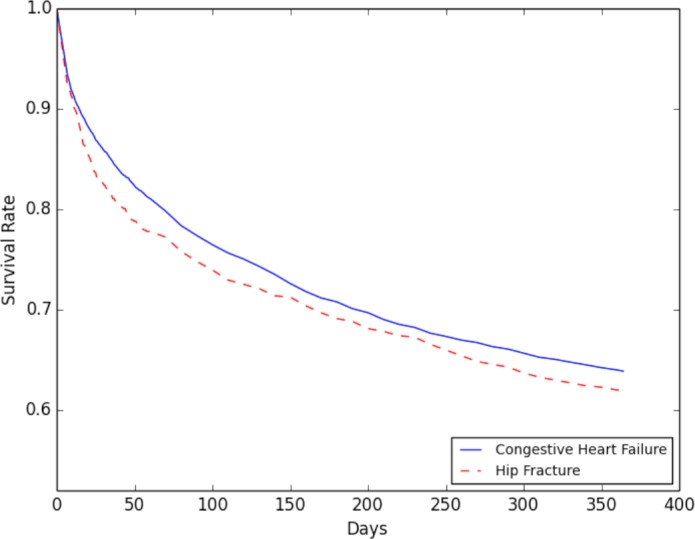
Survival rate for patients within one year from the diagnosis.

Before Discharge Model Results

Before Discharge Model Results

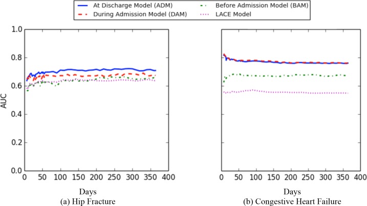
Figure 5 reports on the AUC for predicting the negative outcome within one year using LACE, before admission, during admission, and at discharge) models for hip fracture and CHF patients. The x-axis shows the prediction points at which the model was run, while the y-axis corresponds to the average AUC.

Figure 5.

AUC values for BAM, DAM, and ADM models for outcome prediction within one year.

Across all prediction points, LACE exhibited the lowest AUC values for both cohorts. The before model has similar AUC values as LACE for hip fracture patients, while it has higher AUC than LACE when applied on the CHF cohort. However, the during and at discharge both outperform the LACE and before models. The during model exhibits almost the same AUC as the at-discharge model when predicting the outcome for the CHF patients. By contrast, at discharge model has a higher AUC than the during model for the hip fracture patients.

In both cohorts, the before model had the lowest AUC within the first 20 days. After 20 days, the AUC values increased slightly. The during and at-discharge models exhibited the same trend in performance over time. In CHF, the during model and at-discharge models had the highest AUC during the first two weeks of prediction. Afterwards, the AUC values decline slightly and smoothly until they reach their lowest point at the one-year prediction. By contrast, the AUC values of the during model and at-discharge were the lowest within the first two weeks for the hip fracture patients and increased slightly until they reached their highest AUC values at the one-year prediction.

Post-Discharge Model Results

Next, we analyzed the post-discharge model in two ways: (i) using a single feature representing the days since discharge (post-discharge time), and (ii) all post-discharge data including days since discharge. We analyzed the results in these two phases given the importance of time in the post-discharge model (i.e., the longer you are out of the hospital, the less likely you are to return).

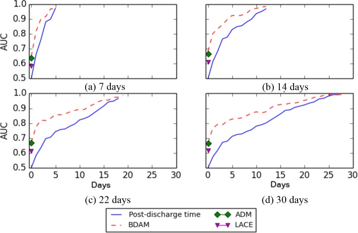
Figure 6 depicts the AUC values for specific checkpoints for the 7, 14, 22, and 30 days prediction points. The x-axis corresponds to the selected checkpoint. The red dashed-line represents the average AUC for post-discharge model at a given checkpoint, while the diamond and triangles correspond to the AUC of at-discharge model and the traditional LACE model, respectively. The blue solid line represents the AUC for the post-discharge time only model. It can be seen that the BDAM model outperformed all models. Moreover, the AUC values increased as additional post-discharge data are included.

Figure 6.

AUC values for BDAM model applied at different successive checkpoints for hip fracture patients at 7, 14, 22 and 30 days negative outcome.

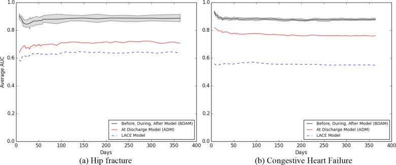
Figure 7 depicts the performance of the LACE, ADM (at discharge) and BDAM (post-discharge) models for different prediction points (where the post-discharge data are averaged across the checkpoints). The upper grey line, lower grey line, and solid black line represent the minimum, maximum, and average AUC, respectively. Both the BDAM and the ADM models performed better than the LACE model by 20 - 30% AUC. In this setting, BDAM had a higher AUC than ADM at all prediction points by 15.8 - 26.5% for hip fracture and 9.7 - 12.1% for CHF patients. Using BDAM, predicting the negative outcome within 7 days had a higher AUC compared to predictions within 30 days.

Figure 7.

Outcome predicting within one year for a) hip fracture and b) CHF.

BDAM results trended differently for the two phenotypes. For hip fracture, the AUC decreased until it reached the lowest values at 21 days, then increased between 21 and 60 days, staying relatively constant afterwards. For CHF, the AUC decreased until 21 days.

Feature Importance

For each prediction point, we retreived the features that, on average, exhibited the highest importance. At all prediction points in both cohorts, days from discharge and days until prediction point displayed the highest importance. The number of appointments after discharge was the third most important predictor for a negative event within 30 days while clinical communication was the forth or fifth important feature within the same time range.

In hip fracture patients, age is one of the top 10 predictors of a negative outcome within 30 days. Diagnosing hip fracture patients with infectious, blood stream, genitouribnary, or circulatory diseases during admission were among the top predictors for readmission within 30 days. In CHF patients, the average number of labs during admission (e.g., creatinine, K, Na, and CO₂) were strong predictors for negative events within 60 days.

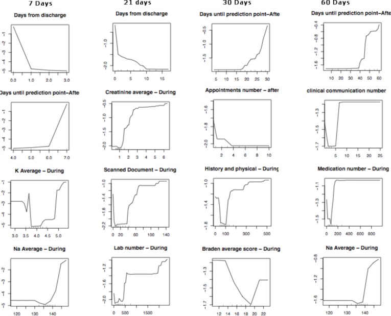
Figure 8 depicts the partial dependency plots for the most important features for 7, 21, 30, and 60 days for hip fracture patients. In the partial dependence plot, the x-axis shows the values of the variable. For a given x value, the

Figure 8.

Partial dependency plots for outcome predictions for hip fracture patients.

y value indicates the probability of the negative outcome after accounting for the values of the other input variables. A small y value indicates a low probability of positive outcome, while a large y indicates a high probability of a positive outcome.

For example, patients who scheduled a small number of appointments after discharge had a higher probability of experiencing a negative outcome. A low and high number appointments scheduled before discharge were associated with a high probability of negative outcome. In addition, a low and high quantity of post-discharge communications had a high probability of a negative outcome. During admission, patients who were prescribed a larger number of medications and lab tests, in comparison to other patients in the cohort, had a higher probability of having a negative outcome. The partial dependency plots of lab values such as K, PVC, and creatinine depict that abnormal values were associated with a high probability of a negative outcome.

Discussion

Predicting negative outcomes and detecting high-risk patients are challenging problems. Our findings demonstrate that including more information about a patient’s post-discharge status may increase the performance of such predictions. This finding is further supported by the observation that the LACE model, while simple to implement, is likely to neglect many key features that can enhance predictions.

One of the critical discoveries made in this study is that the post-discharge time is a strong predictor on its own for a negative outcome. This result affirms the observation that the longer a patient remains out of the hospital, the less likely they will be readmitted at a future point in time. However, time from discharge in isolation lacks important clinical information, which if included, can further improve prediction quality. Moreover, time until prediction quantifies the amount of information collected post-discharge that is not included in time from discharge.

One of the challenges in building and developing the post-discharge model is determining the time period during which post-discharge data should be collected and used for prediction. In this work, we used a random day model. In practice, a post-discharge model can be executed daily to identify high-risk patients, no matter when they were discharged.

Our analysis demonstrates that risk changes over time, especially during the first three months post discharge. In particular, the first 7 to 10 days are the times when frail patients are at high risk of encountering a negative outcome. A decline of the prediction performance over time suggests a variation in recovery stages for healthy patients and a difference in the risk factors for patients who died or were readmitted within the same time frame. For example, the prediction of hip fracture outcome had the lowest performance between 14 and 21 days. Several factors could cause this such as various pre-existing medical problems, the degree of activity, and the ability to attend follow-ups. Further analysis could be done to identify the change in risk factors (e.g. post-discharge complications), and locate the period of time when those factors are correlated with readmission.

Although accurate prediction is crucial, healthcare providers need to identify the values of features that are associated with a higher probability of negative outcome. Locating such values may assist clinicians in understanding the reasons behind a negative outcome, as well as identify early signs of complications. Direct intervention could be applied to lessen risks through outpatient appointments or home visits. In our risk model, the features can be categorized into clinical factors and clinical resources. Both types of features influence predictions at different levels. Specifically, the amount of clinical resources allocated to treat patients before admission and after discharge could identify the patients who have a high probability of encountering a negative outcome. Similarly, the patients who utilized more treatment resources exhibit a higher probability of experiencing a negative outcome except for post-discharge follow-up utilization. A very low utilization value implies the existence of barriers preventing the patient from going to see their healthcare provider. Even low utilization values for some features, such as the number of labs ordered during admission, are associated with negative outcome occurrence. Measuring the unexpected utilization could be leveraged as an indirect method to identify patients who are at high risk.

Conclusions

This study shows that the inclusion of data in EMRs collected post-discharge can improve the performance of negative outcomes predictions, such as readmission or death. This is notable because it shows that traditional readmission prediction models, such as LACE, which focus on information available only at the point of discharge, would benefit with updates over time (provided the information is available). We illustrated that this finding holds true for both acute (i.e., hip fracture) and chronic (i.e., congestive heart failure) patient populations. It is notable that the primary driving factors of our discovery include: 1) time out of the hospital after discharge and 2) information about the quantity of resources allocated for patient that are both physical (e.g. medication, labs, appointments) and electronic (communication, documents).

While our findings are notable, there are several limitations that we wish to acknowledge, which can serve as guidelines for further investigation. First, this study focused on sampling only one day for post-discharge information. A notable extension is evaluating risk scores on multiple consecutive days to identify changes in risk score and identify patients at-risk to apply early intervention. Second, our models neglected the semantics about clinical status that might be documented in communications between patients and their healthcare providers. For instance, patients who communicate they are in severe pain or experiencing complications from opioid medications may miss their follow-ups. Thus, information intimated to care providers may indicate signs of an impending negative outcome. As such, a notable extension to our approach would be to apply natural language processing to detect and characterize such semantics for enhanced modeling. Third, our model represented various features from disparate EHR resources. However, we did not use all patient data such as vital signs (e.g., heart rate or blood pressure), medication doses, changes in laboratory test values, etc. A future direction is to include additional relevant features while accounting for the ratio between sample size and the number of features.

References

- 1.Kansagara D, Englander H, Salanitro A, Kagen D, Theobald C, Freeman M, et al. Risk prediction models for hospital readmission: a systematic review. JAMA. 2011;306(15):1688–98. doi: 10.1001/jama.2011.1515. [DOI] [PMC free article] [PubMed] [Google Scholar]
- 2.Centers for Medicare and Medicaid Services. Readmissions Reduction Program (HRRP) 2016 [Google Scholar]
- 3.AHRQ. Hospital Guide to Reducing Medicaid Readmissions. 2016 [Google Scholar]
- 4.Farrar S, Ryan M, Ross D, Ludbrook A. Using discrete choice modelling in priority setting: an application to clinical service developments. Soc Sci Med. 2000;50(1):63–75. doi: 10.1016/s0277-9536(99)00268-3. [DOI] [PubMed] [Google Scholar]
- 5.Mitton C, Donaldson C. Health care priority setting: principles, practice and challenges. Cost Eff Resour Alloc. 2004;2:3. doi: 10.1186/1478-7547-2-3. [DOI] [PMC free article] [PubMed] [Google Scholar]
- 6.Ben-Chetrit E, Chen-Shuali C, Zimran E, Munter G, Nesher G. A simplified scoring tool for prediction of readmission in elderly patients hospitalized in internal medicine departments. Isr Med Assoc J. 2012;14(12):752–6. [PubMed] [Google Scholar]
- 7.van Walraven C, Dhalla IA, Bell C, Etchells E, Stiell IG, Zarnke K, et al. Derivation and validation of an index to predict early death or unplanned readmission after discharge from hospital to the community. CMAJ. 2010;182(6):551–7. doi: 10.1503/cmaj.091117. [DOI] [PMC free article] [PubMed] [Google Scholar]
- 8.Chen SY, Stem M, Schweitzer MA, Magnuson TH, Lidor AO. Assessment of postdischarge. complications after bariatric surgery: A National Surgical Quality Improvement Program analysis. Surgery. 2015;158(3):777–86. doi: 10.1016/j.surg.2015.04.028. [DOI] [PubMed] [Google Scholar]
- 9.Merkow RP, Ju MH, Chung JW, Hall BL, Cohen ME, Williams MV, et al. Underlying reasons associated with hospital readmission following surgery in the United States. JAMA. 2015;313(5):483–95. doi: 10.1001/jama.2014.18614. [DOI] [PubMed] [Google Scholar]
- 10.Morris MS, Deierhoi RJ, Richman JS, Altom LK, Hawn MT. The relationship between timing of surgical complications and hospital readmission. JAMA Surg. 2014;149(4):348–54. doi: 10.1001/jamasurg.2013.4064. [DOI] [PubMed] [Google Scholar]
- 11.Opheim A, Danielsson A, Murphy MA, Persson HC, Sunnerhagen KS. Early prediction of long-term upper limb spasticity after stroke Part of the SALGOT study. Neurology. 2015;85(10):873–80. doi: 10.1212/WNL.0000000000001908. [DOI] [PMC free article] [PubMed] [Google Scholar]
- 12.Hersh AM, Masoudi FA, Allen LA. Postdischarge environment following heart failure hospitalization: expanding the view of hospital readmission. J Am Heart Assoc. 2013;2(2) doi: 10.1161/JAHA.113.000116. [DOI] [PMC free article] [PubMed] [Google Scholar]
- 13.DeLia D, Tong J, Gaboda D, Casalino LP. Post-discharge follow-up visits and hospital utilization by medicare patients. Medicare Medicaid Res Rev. 2014;4(2):2007–2010. doi: 10.5600/mmrr.004.02.a01. [DOI] [PMC free article] [PubMed] [Google Scholar]
- 14.Hernandez AF, Greiner MA, Fonarow GC, Hammill BG, Heidenreich PA, Yancy CW, et al. Relationship between early physician follow-up and 30-day readmission among Medicare beneficiaries hospitalized for heart failure. JAMA. 2010;303(17):1716–22. doi: 10.1001/jama.2010.533. [DOI] [PubMed] [Google Scholar]
- 15.Jackson C, Shahsahebi M, Wedlake T, DuBard CA. Timeliness of outpatient follow-up: an evidence-based approach for planning after hospital discharge. Ann Fam Med. 2015;13(2):115–22. doi: 10.1370/afm.1753. [DOI] [PMC free article] [PubMed] [Google Scholar]
- 16.Sharma G, Kuo Y-F, Freeman JL, Zhang DD, Goodwin JS. Outpatient follow-up visit and 30-day emergency department visit and readmission in patients hospitalized for chronic obstructive pulmonary disease. Arch Intern Med. 2010;170(18):1664–70. doi: 10.1001/archinternmed.2010.345. [DOI] [PMC free article] [PubMed] [Google Scholar]
- 17.CDC. International Classification of Diseases, Ninth Revision, Clinical Modification (ICD-9-CM) 2011 [PubMed] [Google Scholar]
- 18.ScikitLearn. 2016. Available from: http://scikit-learn.org/stable/modules/generated/sklearn.ensemble.RandomF orestClassifier.html.