A Vector Uniform Cramer-Rao Bound for SPECT System Design

Abstract

In this paper, we present the use of modified uniform Cramer-Rao type bounds (MUCRB) for the design of single photon emission tomography (SPECT) systems. The MUCRB is the lowest attainable total variance using any estimator of an unknown vector parameter, whose mean gradient matrix satisfies a given constraint. Since the mean gradient is closely related to local impulse function, the MUCRB approach can be used to evaluate the fundamental tradeoffs between spatial resolution and variance that are achievable with a given SPECT system design. As a possible application, this approach allows one to compare different SPECT system designs based on the optimum average resolution-variance tradeoffs that can be achieved across multiple control-points inside a region-of-interest. The formulation of the MUCRB allows detailed modelling of physical aspects of practical SPECT systems and requests only a modest computation load. It can be used as an analytical performance index for comparing different SPECT system or aperture designs.

I. Introduction

Single photon emission computerized tomography (SPECT) permits in vivo mapping of radio-labeled molecules in small animals. Compared to positron emission tomography (PET), SPECT can offer a better spatial resolution [1]–[6]. It also enjoys a wider variety of tracers and allows simultaneous multiple tracer studies. One of the key challenges for ultrahigh resolution SPECT design is to achieve a reasonable balance between resolution and detection efficiency. Several recent efforts for the design and modeling of SPECT systems have been reported by Cao et al. [7], Meikle et al. [8], Schramm et al. [9], Song et al. [10], Beekman et al. [11], Van der Have et al. [12].

Monte Carlo (MC) simulation is the most widely used approach for SPECT system and aperture designs. It allows detailed modeling and comprehensive evaluations of a given design. However, MC studies are often time-consuming, especially for evaluating the noise characteristics offered by a given system. To overcome this problem, many analytical methods have been developed. Rentmeester et al. have presented an analytical model for optimizing an ultra-high resolution small animal SPECT system [13]. Bal et al. have reported a geometric-criteria based optimization method for optimizing the arrangement of pinholes [14]. Accorsi et al. have used signal-to-noise ratio (SNR) as a design criterion for selecting coded-aperture patterns [15]. In general, analytical methods often rely on simplified system models that lead to a greatly improved computation efficiency. This allows one to search through the multivariate system parameter space with a reasonable computation load. With a well characterized physical configuration, knowledge on noise statistics and a stochastic object model, an imaging system can also be evaluated based on its performance for specific imaging tasks, such the lesion detection [16]–[22]. Detailed discussions on task based image quality assessment and its applications in system design and optimization were given by Barrett et al. [23].

SPECT systems may also be evaluated based on the fundamental tradeoffs between spatial resolution and image noise that can be achieved in reconstructed images. Such tradeoffs may be derived analytically using the Cramer-Rao (CR) type bounds [24]. The ordinary CR bound is applicable to unbiased estimators only. This limits its use in imaging problems, since estimator bias is typically inevitable. The uniform Cramer-Rao bound (UCRB), developed by Hero et al. [25], [26], provides the smallest attainable variance with any estimator whose bias gradient satisfies a certain constraint. Since bias gradient is an indirect measure of imaging resolution, one may plot the UCRB against the norm of the corresponding bias gradient vector. This leads to the so-called resolution-variance tradeoff curve. An example of using the UCRB for evaluating SPECT systems was presented by Hua et al. [27]. In this work, Compton cameras were compared with mechanically collimated gamma cameras for SPECT imaging applications. Furthermore, UCRB approach provides the optimum tradeoffs between voxel-wise resolution and variance, which is independent of the estimator used. One of the key problems of this approach is that the bias gradient norm constraint was inadequate for determining spatial resolution function. For example, point-spread functions with very different FWHM and FWTM values may satisfy the same bias gradient norm constraint [28]. Therefore, the relationship between bias gradient norm and variance may not represent the true tradeoff between imaging resolution and variance.

To overcome this limitation, we have previously proposed a modified uniform Cramer-Rao bound (MUCRB) [29]. It follows the same notation as in Hero’s formulation, but with a key difference. The MUCRB uses a resolution constraint that is applied on the mean gradient rather than the bias gradient of an estimator. The MUCRB offers two benefits over the original UCRB by Hero. Firstly, mean gradient is closely related to the linearized local impulse response (LIR) function [30]. The latter is widely used to describe spatial resolution property in images. Therefore, the MUCRB allows one to compare the true resolution-variance tradeoff that is attainable with given imaging system designs. Secondly, for linear Gaussian and linear Poisson problems, the MUCRB can be achieved (asymptotically) with post-filtered penalized maximum likelihood estimators (PF-PML) that are widely used in routine practice. In our previous studies, the use of the MUCRB has provided reasonable predictions in comparing different SPECT aperture designs [29], [31].

However, the formulation of the MUCRB in [29] is limited to the scalar estimation problem. It gives the minimum variance attainable with any estimator of a scalar function of a vector parameter, e.g. the tracer uptake in a single voxel in an image. From a practical view point, one may be more interested in the estimation of a vector function of underlying unknown parameters. For example, SPECT systems are normally designed to provide simultaneous estimate of tracer uptakes in multiple voxels. In this paper, we extended the MUCRB [29] into the vector estimation case using a similar approach as previously discussed by Eldar in [32]. This vector MUCRB allows the evaluation of the minimum achievable total (or average) variance over an arbitrary set of voxels, given that the spatial resolution functions achieved at these voxels satisfy a certain constraint. This development provides a general form of UCRB that incorporates the original UCRB by Hero et al. and the scalar MUCRB [19] as special cases. This offers a more meaningful way to compare the resolution-variance tradeoffs achieved with different systems.

In the following text, we will provide a brief review of the scalar MUCRB developed in [1], followed by the derivation of the vector MUCRB. The use of the vector MUCRB for SPECT system design will be demonstrated with a Monte Carlo example.

II. Methods

A. Modified Uniform Cramer-Rao Bounds for Aperture Design

1) The Scalar MUCRB

The spatial resolution property of an estimator can be quantified using the linerized local-impulse response (LIR) function [30]. Let x = [x₁, x₂,..., x_N]^T ∈ R^N denote the set of unknown deterministic parameters, e.g., object intensities underlying the projection data y. The mapping from x to y is governed by a conditional probability density function p(y;x). In the context of emission tomography, y is a collection of random Poisson (or Gaussian) variables. Its expectation is given by the following transform

$$\overline{\mathit{y}}=\mathit{A}·\mathit{x}+\mathit{r},$$ (1)

where A is the system-response matrix and r denotes extra noise components. x̂ = [x̂₁, x̂₂, ···, x̂_N]^T denotes an estimator of the underlying image function, whose mean is

$$\mu (\mathit{x})\equiv E_{\mathit{x}}[\widehat{\mathit{x}}]=\int \widehat{\mathit{x}}(\mathit{y})·p(\mathit{y};\mathit{x})·d\mathit{y},$$ (2)

where E_x[x̂] is the expectation of the estimator x̂ for a given deterministic variable x. The linearized LIR for the j’th voxel is defined as [30]

$$\begin{array}{l}{\mathit{l}}_j(\mathit{x})=\underset{\delta \to 0}{lim}\frac{\mu (\mathit{x}+\delta e_j)-\mu (\mathit{x})}{\delta }=\partial \mu (\mathit{x})/\partial x_j\\ =\partial E_{\mathit{x}}(\widehat{\mathit{x}})/\partial x_j\\ ={[\partial E_{\mathit{x}}({\widehat{x}}_1)/\partial x_j,\partial E_{\mathit{x}}({\widehat{x}}_2)/\partial x_j,\cdots \cdots ,\partial E_{\mathit{x}}({\widehat{x}}_N)/\partial x_j]}^T.\end{array}$$ (3)

For the scalar MUCRB shown in [29], we proposed a resolution constraint that is applied on the mean gradient vector corresponding to a given voxel,

$$\begin{array}{l}{\mathit{g}}_j={\nabla }_{\mathit{x}}[E_{\mathit{x}}({\widehat{x}}_j)]\\ ={[\partial E_{\mathit{x}}({\widehat{x}}_j)/\partial x_1,\partial E_{\mathit{x}}({\widehat{x}}_j)/\partial x_2,\cdots \cdots ,\partial E_{\mathit{x}}({\widehat{x}}_j)/\partial x_N]}^T.\end{array}$$ (4)

It is easily seen that l_j and g_j defined in (3) and (4) are closely related. They become identical if the mean gradient matrix (as defined later in (10)) is symmetric. Suppose we know a priori that the desired point-spread function (or the mean gradient vector) at the j’th voxel is f_j. A possible way to chose an appropriate estimator (x̂) is to limit our choice to those that have their mean gradient (g_j) vector ssatisfying a similarity constraint

$${\Vert {\mathit{g}}_j-{\mathit{f}}_j\Vert }_{\mathit{C}}\le \gamma ,$$ (5)

where γ is a threshold that governs the degree of similarity between f_j and g_j. C is a symmetric and positive definite weighting matrix. ||.|| is the Euclidean norm of a vector, so that

$${\Vert {\mathit{g}}_j-{\mathit{f}}_j\Vert }_{\mathit{C}}^2={({\mathit{g}}_j-{\mathit{f}}_j)}^T·\mathit{C}·({\mathit{g}}_j-{\mathit{f}}_j).$$ (6)

Since g_j is closely related to the local impulse response function, all estimators that satisfy constraint (5), with a small γ, would produce very similar spatial resolution properties, regardless the physical system configuration and the estimation method used. With this constraint in place, a possible strategy for system optimization is to choose the system design that leads to the minimum attainable variance on the target voxel. In [29], we have demonstrated that the minimum variance on the j’th voxel achievable with any biased estimator, whose mean gradient vector satisfies (5), is given by a scalar MUCRB as

$$\mathit{Var}({\widehat{x}}_j)\ge {\mathit{f}}_j^T·{[\mathit{J}+{(\lambda ·\mathit{C})}^{-1}]}^{-1}·\mathit{J}·{[\mathit{J}+{(\lambda ·\mathit{C})}^{-1}]}^{-1}·{\mathit{f}}_j.$$ (7)

where γ is a scalar constant. The mean-gradient vector of the efficient estimator that achieves this bound is given by

$${\mathit{g}}_{\mathit{optimum}}=\mathit{J}·{[\mathit{J}+{(\lambda ·\mathit{C})}^{-1}]}^{-1}·{\mathit{f}}_j,$$ (8)

where J is the Fisher information matrix (FIM) that is defined as

$$\mathit{J}=E\left\{\left[\frac{\partial logp(\mathit{y};\mathit{x})}{\partial \mathit{x}}\right]·{\left[\frac{\partial logp(\mathit{y};\mathit{x})}{\partial \mathit{x}}\right]}^T\right\}.$$ (9)

2) A Vector MUCRB

With the scalar MUCRB (7), one can derive the optimum voxel-wise resolution-variance tradeoffs attainable with any estimator of a scalar function of a vector parameter (such as the true image vector). However, for evaluating an imaging system, we are normally interested in estimating multiple components of x (or a vector function of x) simultaneously. For example, an ultrahigh resolution SPECT may be designed to provide an optimized performance for imaging an region-of-interest (ROI). Therefore, it is desirable to have a MUCRB that allows the evaluation of average or collective resolution-variance tradeoffs, when the imaging task is to estimate a vector function of the underlying parameter x. For this purpose, we extend the scalar MUCRB (6) into the vector estimation case. This extension is similar to the derivation given by Eldar in [32]. For the estimation problem outlined in the previous section, the mean gradient matrix of an estimator is defined as

$$\begin{array}{l}\mathit{G}=\frac{\partial E_{\mathit{x}}[\widehat{\mathit{x}}]}{\partial \mathit{x}}\\ =\left\{\begin{array}{cccc}\frac{\partial }{\partial x_1}{E}_{\mathit{x}}[{\widehat{x}}_1]& \frac{\partial }{\partial x_2}{E}_{\mathit{x}}[{\widehat{x}}_1]& \cdots & \frac{\partial }{\partial x_N}{E}_{\mathit{x}}[{\widehat{x}}_1]\\ \frac{\partial }{\partial x_1}{E}_{\mathit{x}}[{\widehat{x}}_2]& \frac{\partial }{\partial x_2}{E}_{\mathit{x}}[{\widehat{x}}_2]& \cdots & \frac{\partial }{\partial x_N}{E}_{\mathit{x}}[{\widehat{x}}_2]\\ ⋮& ⋮& \ddots & ⋮\\ \frac{\partial }{\partial x_1}{E}_{\mathit{x}}[{\widehat{x}}_N]& \frac{\partial }{\partial x_2}{E}_{\mathit{x}}[{\widehat{x}}_N]& \cdots & \frac{\partial }{\partial x_N}{E}_{\mathit{x}}[{\widehat{x}}_N]\end{array}\right\}.\end{array}$$ (10)

Each row of G is the mean gradient vector for a given voxel in the image and each column is the local-impulse response (LIR) function (or point-spread function) as defined in (3). If the mean gradient matrix G is symmetric, the mean-gradient vector is equal to the LIR for the same voxel. For an arbitrary estimator x̂, whose mean gradient matrix is G, its covariance matrix must satisfy [24],

$$\mathit{Cov}\{\widehat{\mathit{x}}\}\ge \mathit{G}·{\mathit{J}}^{-1}·{\mathit{G}}^T.$$ (11)

Suppose the desired spatial resolution function in reconstructed images is known, we may represent it as a matrix F. Each row of F is the desired (or target) mean-gradient vector for a given voxel. As the first step towards the vector MUCRB, we chose a subset of estimators that have their corresponding mean gradient metrics satisfy an “average” resolution constraint defined as

$$s=tr\left[\mathit{W}·(\mathit{G}-\mathit{F})·\mathit{C}·{(\mathit{G}-\mathit{F})}^T·{\mathit{W}}^T\right]\le \gamma ,$$ (12)

where C is a positive definite matrix and W is a nonnegative definite weighting matrix. It is easily seen that the scalar s is basically a weighted average over all Euclidean distances between true and target mean gradient vectors for all voxels in the FOV. One of the applications for this development is to optimize SPECT systems for imaging a ROI, ℜ. For this task, matrix W may be defined as

$$\mathit{W}=\mathit{diag}\{w_j\},w_j=\{\begin{array}{ll}1\hfill & j\in \mathfrak{R}\hfill \\ 0\hfill & \mathit{otherwise}\hfill \end{array}.$$ (13)

If (12) is satisfied with a small threshold value γ, the resolution properties for all voxels in the ROI should be close to the desired ones as specified by matrix F. Note that the positive-definite matrix C can be used to control the actual definition of the similarity between the target and actual PSFs. For example, it may be so chosen that the differences in the tail region carry greater weight in the Euclidean distance. Therefore actual PSFs that are wider and narrower than the target PSF could get differently-weighted results in the calculation of the similarity using (12). Therefore actual PSFs that are wider and narrower than the target PSF could get different penalties in the calculation of the similarity using (12).

For any arbitrary estimator that has a given mean-gradient matrix G, the minimum achievable total variance across all voxels in the ROI is given by the biased CRB [30],

$$V_{\mathit{tot}}\ge tr[\mathbf{W}·\mathit{Cov}(\widehat{\mathbf{x}})·\mathbf{W}]=tr[\mathbf{W}·\mathbf{G}·{\mathbf{J}}^{-1}·{\mathbf{G}}^T·{\mathbf{W}}^T].$$ (14)

Eq. (14) is less useful since it is specific to a very restrictive set of estimators, whose mean gradient vectors are given by G. To obtain a more useful bound, we find the lowest attainable total variance by any estimator that has its mean gradient matrix satisfies (12), by constrained minimization

$$V_{min}\ge \underset{s\le \gamma }{argmin}(V_{\mathit{tot}})=\underset{s\le \gamma }{argmin}(tr[\mathbf{W}·\mathbf{G}·{\mathbf{J}}^{-1}·{\mathbf{G}}^T·{\mathbf{W}}^T]).$$ (15)

V_min can be evaluated by forming a Lagrange as

$$L=Tr[\mathit{W}·\mathit{G}·{\mathit{J}}^{-1}·{\mathit{G}}^T·{\mathit{W}}^T]+\lambda \left\{Tr\left[\mathit{W}·(\mathit{G}-\mathit{F})·\mathit{C}·{(\mathit{G}-\mathit{F})}^T·{\mathit{W}}^T\right]-\gamma \right\}.$$ (16)

Since L is strictly convex, the optimum mean gradient G that minimizes L can be found by setting the derivative of (16) to 0,

$$\begin{array}{l}\frac{d}{d\mathit{G}}L=\frac{d}{d\mathit{G}}\left[Tr[\mathit{W}·\mathit{G}·{\mathit{J}}^{-1}·{\mathit{G}}^T·{\mathit{W}}^T]+\lambda ·\left\{Tr\left[\mathit{W}·(\mathit{G}-\mathit{F})·\mathit{C}·{(\mathit{G}-\mathit{F})}^T·{\mathit{W}}^T\right]-\gamma \right\}\right]\\ =0.\end{array}$$ (17)

Since

$$\begin{array}{l}\frac{d}{d\mathit{G}}\left\{Tr[\mathit{W}·\mathit{G}·{\mathit{J}}^{-1}·{\mathit{G}}^T·{\mathit{W}}^T]\right\}={\mathit{W}}^T·\mathit{W}·\mathit{G}·{({\mathit{J}}^{-1})}^T+{\mathit{W}}^T·\mathit{W}·\mathit{G}·{\mathit{J}}^{-1}\\ =2·{\mathit{W}}^T·\mathit{W}·\mathit{G}·{\mathit{J}}^{-1}\\ =2·\mathit{W}·\mathit{G}·{\mathit{J}}^{-1},\end{array}$$ (18)

and

$$\frac{d}{d\mathit{G}}\left\{tr\left[\mathit{W}·(\mathit{G}-\mathit{F})·\mathit{C}·{(\mathit{G}-\mathit{F})}^T·{\mathit{W}}^T\right]\right\}=2·\mathit{W}·(\mathit{G}-\mathit{F})·\mathit{C},$$ (19)

one can substitute (18) and (19) into (17) and obtain

$$\frac{d}{d\mathit{G}}L=2·\mathit{W}·\mathit{G}·{\mathit{J}}^{-1}+\lambda ·2·\mathit{W}·(\mathit{G}-\mathit{F})·\mathit{C}=0.$$ (20)

Assuming that J is non-singular, the optimum mean gradient matrix G must satisfy

$$\mathit{W}·\mathit{G}=\lambda ·\mathit{W}·\mathit{F}·{[\mathit{J}+{(\lambda \mathit{C})}^{-1}]}^{-1}·\mathit{J}.$$ (21)

Note that

$$\mathbf{G}=\lambda ·\mathbf{F}·{[\mathbf{J}+{(\lambda \mathbf{C})}^{-1}]}^{-1}·\mathbf{J}$$ (22)

is a sufficient condition for (21) to hold.

Substitute (21) into (14), the minimum achievable total variance, with any estimator that has a mean gradient matrix satisfies (12), is given by

$$\begin{array}{l}{V}_{min}\ge \underset{s\ge \gamma }{argmin}(V_{\mathit{tot}})\\ =\underset{s\le \gamma }{argmin}(tr[\mathbf{W}·\mathbf{G}·{\mathbf{J}}^{-1}·{\mathbf{G}}^T·{\mathbf{W}}^T])\times tr\left\{\left[\mathbf{W}·\mathbf{F}·{\left(\frac{1}{\lambda }{\mathbf{C}}^{-1}+\mathbf{J}\right)}^{-1}·\mathbf{J}\right]·{\mathbf{J}}^{-1}·{\left[\mathbf{W}·\mathbf{F}·{\left(\frac{1}{\lambda }{\mathbf{C}}^{-1}+\mathbf{J}\right)}^{-1}·\mathbf{J}\right]}^T\right\}\\ =tr\left\{\mathbf{W}·\mathbf{F}·{[\mathbf{J}+{(\lambda \mathbf{C})}^{-1}]}^{-1}·\mathbf{J}·{[\mathbf{J}+{(\lambda \mathbf{C})}^{-1}]}^{-1}·{\mathbf{F}}^T·{\mathbf{W}}^T\right\}.\end{array}$$ (23)

Note that the modified UCRBs (7) and (23) are similar, in nature, to the uniform Cramer-Rao bound (UCRB) originally proposed by Hero [25], [26]. In fact, (7) becomes identical to the original UCRB by Hero if one chooses the desired mean gradient vector f_j to be the unit vector e_j. The vector MUCRB (23) incorporates two major improvements to account for the intrinsic limitations of Hero’s formulation. It incorporates a more accurate constraint of spatial resolution and allows the extension from a voxel-wise performance index into a measure of the average resolution/variance tradeoff across an arbitrarily defined ROI. The formulations for the UCRBs discussed so far are summarized in Table I.

TABLE I.

Summary of Formulations for the Uniform Cramer-Rao Bounds

	UCRBs for single voxel estimation		UCRB for vector estimation
	The original UCRB by Hero [31],[32]	Modified Scalar UCRB [35]	Modified Vector UCRB
Resolution Constraint	||dj||C = [gj − ej] · C · [gj − ej] ≤ γ	||gj − fj||C ≤ γ	tr⌊W ·(G − F) · C · (G − F)T · WT ⌋ ≤ γ
The minimum achievable variance	Var(x̂j) ≥ [J + (λ · C)−1]−1 · J · [J + (λ · C)−1]	Var(x̂j) ≥ ej · FT · [J + (λ · C)−1]−1 · J · [J + (λ · C)−1] · F · ej	Vartotal ≥ tr[W · F · [(λ · C)−1 + J]−1 · J · [(λ · C)−1 + J]−1 · FT · WT]
Efficient estimators	PML estimator with quadratic penalty function R(x) that satisfies C−1 = ∇2R(x)	Post-filtered PML estimator with the desired resolution function.
Mean of the efficient estimator	E(x̂j) ≈ ejT · {[J + (λ · C)−1]}−1 · A · Σ−1 · ȳ	E(x̂) ≈ FT · {[J + (λ · C)−1]}−1 · A · Σ−1 · ȳ
Optimum mean/bias gradient vectors	dj ≈ {[J + (λ · C)−1]}−1 · J · ej	gj ≈ {[J + (λ · C)−1]}−1 · J · fj	G ≈ F · [J + (λC)−1] −1 · J

3) Achievability of the MUCRBs

In general, there is no guarantee that an estimator exists to achieve the MUCRBs given by (7) and (23). However, in special cases such as the linear Gaussian model, a post-filtered penalized weighted least-square estimator (or equivalently, the post-filtered penalized maximum likelihood estimator)

$$\{\begin{array}{l}{\widehat{\mathbf{x}}}_{\mathbf{PWLS}}=\underset{\mathbf{x}}{argmax}[log\mathbf{p}(\mathbf{x};\mathbf{y})-\beta R(\mathbf{x})]\hfill \\ =\underset{\mathbf{x}}{argmax}\left[-\frac{\mathbf{1}}{\mathbf{2}}{(\mathbf{y}-\mathbf{Ax})}^{\prime }{\mathbf{\sum }}^{-\mathbf{1}}(\mathbf{y}-\mathbf{Ax})-\beta R(\mathbf{x})\right]\hfill \\ \mathit{and}\mathit{then}\hfill \\ {\widehat{\mathbf{x}}}_{\mathbf{PF}-\mathit{PWLS}}=\mathbf{F}·{\widehat{\mathbf{x}}}_{\mathit{PWLS}}(\mathbf{y}),\hfill \end{array}$$ (24) (25)

is shown to achieve the bound (23), with the quadratic penalty function R(x) given by

$${\mathbf{C}}^{-1}={\nabla }^{2}R(\mathbf{x}).$$ (26)

Σ is the covariance matrix of the data y and β in (23) is chosen to be 1/λ [29], [32], [33]. It has also been shown that the MUCRBs (7) and (23) can be achieved asymptotically with penalized maximum likelihood estimators for the linear Poisson model that better describes the data acquisition process in emission tomography. Note that these conclusions follow easily from Eq. 22 in [32] and Eq. 60 in [33]. So the proof for the achievability of the vector MUCRB is ignored in this text. These discussions also indicated the (asymptotic) optimality of the PF-PWLS (or PF-PML) estimators. For linear Gaussian models shown in (1), if the desired mean-gradient matrix (or LIR) is known, the PF-PML estimator provides the minimum achievable total variances over an arbitrarily chosen subset of voxels. A few remarks on the vector MUCRB are provided below:

• The choice of the target PSF. It is worth noting that the optimum choice of the target PSF depends on the particular imaging task chosen. Since an imaging system is typically designed for a range of applications, one may choose to use some “general” forms of PSF (such as Gaussian function) for the first-order comparison. However, the formulation derived allows one to use any desired PSF function. The vector MUCRB can be adapted to more specific applications, for which the desired PSF may be known a priori. In such case, these formulations will not only predict the minimum achievable total variance, but also identify the efficient estimator that can be used to achieve the limit. As previously discussed, the optimum performance, measured by the tradeoffs between the average resolution and the average variance over multiple points, can be achieved (asymptotically) with the popular post-filtered penalized likelihood estimators. This adds to the practicality of the vector MUCRB for system design and comparison.

• The similarity measure (12) and the actual resolution function. For SPECT system design, the preferred scenario for applying the vector MUCRB is to measure the average resolution-variance tradeoffs in relatively homogeneous regions. If the actual image properties are very different from point to point, the weighting over multiple relatively different PSFs may be problematic. In such case, since the Euclidean distances corresponding to different points are simply added together, this total distance may be dominated by the component for a particular point in the image. This makes it difficult to come up with a meaningful “average” resolution measure as required by the vector MUCRB method. We acknowledge that this is a potential question for the vector MUCRB approach. Fundamentally, similar difficulties are inevitable if one tries to quantify the resolution functions over multiple points using a single scalar. Given the multivariate nature of the PSFs, it is simply impossible to fully describe the resolution properties using a single value. In any case, a sensible system evaluation is likely to take several studies, each with a different performance index focused on a single imaging task.

4) Implementation of the Vector MUCRB for System Design

The recipe for computing the MUCRB (7) has previously been described in [26], [29]. In stead of deriving the MUCRB for each threshold value γ, one can vary the value of the Lagrange multiplier λ and trace out a resolution-variance tradeoff curve. This involves the use of the conjugate-gradient method [40] for solving simultaneous equations [J + (λ · C)⁻¹] · z = f. A similar approach was used to derive the vector MUCRB (23). For each given F, the efficient estimator (21) and the MUCRB (23) can be derived by solving the following simultaneous equations:

$$\left\{\begin{array}{cccc}\mathbf{J}+{(\lambda ·\mathbf{C})}^{-1}& 0& 0& 0\\ 0& \mathbf{J}+{(\lambda ·\mathbf{C})}^{-1}& 0& 0\\ 0& 0& \ddots & 0\\ 0& 0& 0& \mathbf{J}+{(\lambda ·\mathbf{C})}^{-1}\end{array}\right\}\times \left\{\begin{array}{c}{\mathbf{z}}_1\\ {\mathbf{z}}_2\\ ⋮\\ {\mathbf{z}}_n\end{array}\right\}=\left\{\begin{array}{c}{\mathbf{f}}_1\\ {\mathbf{f}}_2\\ ⋮\\ {\mathbf{f}}_n\end{array}\right\},$$ (27)

where f_j’s are the column vectors of matrix F that are corresponding to non-zero diagonal elements of W. Eq. (27) was solved with a C code that are based on the routine given in [40]. The vector MUCRB (23) can be given as

$$\begin{array}{l}{V}_{min}\ge tr\left\{\mathbf{W}·\mathbf{F}·{[\mathbf{J}+{(\lambda \mathbf{C})}^{-1}]}^{-1}·\mathbf{J}·{[\mathbf{J}+{(\lambda \mathbf{C})}^{-1}]}^{-1}·{\mathbf{F}}^T·{\mathbf{W}}^T\right\}\\ =tr\{{\{\begin{array}{cccc}{\mathbf{z}}_1& {\mathbf{z}}_2& \cdots & {\mathbf{z}}_n\end{array}\}}^T·\mathbf{J}·\{\begin{array}{cccc}{\mathbf{z}}_1& {\mathbf{z}}_2& \cdots & {\mathbf{z}}_n\end{array}\}\}.\end{array}$$ (28)

For a practical SPECT system, matrix [J + (λ · C)⁻¹] is normally very large, even when the sparseness of the system response is taken into account. To facilitate the calculation of the MUCRB, we have developed a parallel computation strategy that performs the forward projection step ([J + (λ · C)⁻¹] · z) simultaneously with multiple CPUs.

As shown in (21), for a given physical system design and a given deterministic image function, there are two factors that affect the spatial resolution function of the optimum estimator. These are the regularization term (λ · C)⁻¹ and the filter function F. In order to derive the resolution-variance tradeoff curve, we chose to use a small regularization factor (β = 1/λ = 10⁻¹⁴ for the simulation outlined below). R(x) used was the uniform quadratic roughness penalty function as defined in Section IV in [30]. Therefore, the resolution property offered by the optimum estimator is determined mainly by the filter function F. As previously discussed, each column of F defines the desired PSF (or more precisely the main gradient function) corresponding to a given voxel. In this study, these columns were defined based on spatially shifted 3-D Gaussian functions of uniform width. By varying the shape or width of these PSFs, one can evaluate different tradeoffs between the minimum attainable total variance and spatial resolution function that are given by the corresponding mean gradient matrix.

Using (21) and (23), we evaluated several resolution-variance tradeoff curves for comparing different system configurations. These are summarized as the following:

• Point-wise resolution/variance tradeoffs. It is the tradeoffs between the minimum achievable variance on a given voxel derived with (7) and the FWHM of the corresponding point-spread function given by (8).

• Point-wise contrast-recovery/variance tradeoffs. The contrast recovery coefficient (CRC) of local impulse response is an alternative measure of the spatial resolution achieved at a given voxel [34], [35]. It measures how much “energy” was recovered back to the voxel that contains the original point impulse. The tradeoffs between CRC and point-wise variance may also be viewed as a signal-to-noise ratio. It relates the fraction of the impulse signal put back to the voxel by reconstruction and the image noise at the same voxel.

• Average resolution-variance tradeoffs. For an ROI that consists of multiple voxels-of-interest, the average variance over these voxels is derived using (23). The point spread functions at these voxels can be obtained using (21). Since the post-filtering process normally leads to PSFs that are similar in shape, we used a simple process to derive the average resolution. LIRs corresponding to all voxels were shifted to the center of the FOV and summed together to form an “average LIR”. Its FWHM was used as the “average” resolution over all voxels-of-interest. In this simulation study, the average resolution-variance tradeoff curves were compared with their voxel-wise counterparts for a simulated SPECT system.

• Bias-variance curve for ROI quantitation.total uptake may also be viewed as a measure of spatial resolution in a broader sense. The total activity uptake inside a ROI is given by

  $$t(\widehat{\mathbf{x}})=\sum _{i\in \mathit{ROI}}{\widehat{x}}_i=w^T·\widehat{\mathbf{x}},$$ (29)
  where w is an indicator vector defined as

  $$w={\{w_j\}}^T,w_j=\{\begin{array}{ll}1\hfill & j\in \mathit{ROI}\hfill \\ 0\hfill & \mathit{otherwise}\hfill \end{array}.$$ (30)
  Using the equation for mean estimators as shown in Table I, the expectation of t(x̂) is computed as

  $$\begin{array}{l}\mu [t(\widehat{\mathbf{x}})]\approx w^T·{\mathbf{F}}^T·{\{[\mathbf{J}+{(\lambda ·\mathbf{C})}^{-1}]\}}^{-1}·{\mathbf{A}}^T·{\mathbf{\sum }}^{-1}·\overline{\mathbf{y}}\\ =w^T·{\mathbf{F}}^T·{\{[\mathbf{J}+{(\lambda ·\mathbf{C})}^{-1}]\}}^{-1}·\mathbf{J}·\mathbf{x}.\end{array}$$ (31)
  The mean bias for ROI quantitation is therefore

  $$\mathit{bias}[t(\widehat{\mathbf{x}})]\approx w^T·{\mathbf{F}}^T·{\{[\mathbf{J}+{(\lambda ·\mathbf{C})}^{-1}]\}}^{-1}·\mathbf{J}·\mathbf{x}-w^T·\mathbf{x}.$$ (32)
  With the efficient estimator that achieves the minimum total variance (23), the variance associated with the total activity in the ROI is

  $$V_{\mathit{ROI}}=w^T·\mathbf{W}·\mathbf{F}·{[\mathbf{J}+{(\lambda \mathbf{C})}^{-1}]}^{-1}·\mathbf{J}·{[\mathbf{J}+{(\lambda \mathbf{C})}^{-1}]}^{-1}·\mathbf{F}·\mathbf{W}·w.$$ (33)
  In this study, W was chosen to be the identity matrix. The variance of t(x̂) is given as

  $$V_{\mathit{ROI}}=w^T·\mathbf{F}·{[\mathbf{J}+{(\lambda \mathbf{C})}^{-1}]}^{-1}·\mathbf{J}·{[\mathbf{J}+{(\lambda \mathbf{C})}^{-1}]}^{-1}·\mathbf{F}·w.$$ (34)

  This equation is identical to (17) previously given in [36]. By varying the width of the desired PSF (column vectors of F), one can derive the tradeoffs between the mean bias and the corresponding variance for ROI qnantitation.

B. Monte Carlo Simulation of a SPECT System

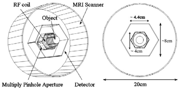
The MUCRB approach was evaluated in the design of a MRI compatible SPECT system [37]. It is based on the use of an energy-resolved photon counting (ERPC) semiconductor detector that we are developing. This detector has an active area of roughly 4.5 cm × 4.5 cm, divided into 128 × 128 pixels of 350μm each. In this simulation, four detectors having similar total dimensions but with different pixelation configurations were compared. These detectors have 44 × 44, 90 × 90, 128 × 128 and 220 × 220 square pixels of 1 mm, 0.5 mm, 0.35 mm and 0.2 mm in size respectively. All detectors were assumed to be 100% efficient for detecting I-125 gamma rays. The depth-of-interaction (DOI) effect was not modeled in this simulation. Six detectors were used to form a stationary ring. The collimator system consists of 6 apertures that are made of tungsten sheet of 5 mm in thickness. Each aperture has 4 × 4 to 9 × 9 pinholes of 200 μm in diameter. As a basic design rule, the pinholes locations were so chosen that (a) the overlapping between projections through multiple pinholes was minimized and (b) the entirely detector area are fully utilized by the projections. Design parameters of several apertures are given in Table II. All pinholes have sharp knife-edges and acceptance cones of 90 degrees on both sides. Photon scattering and penetration in aperture were not modeled. The imaging study was based on a simulated phantom that has a cylindrical volume of 1 cm long and 1 cm in diameter. It was divided into or 64 × 64 × 64 or 128 × 128 × 128 voxels. Each voxel was 200 μm × 200 μm × 200 μm or 100 μm × 100 μ × 100 μm in size. The source contains a total activity of 100 μCi. The phantom consists of two hot spherical volume of 1 mm in diameter and two hot ellipsoidal volumes that have half-axes of 0.4 mm, 0.4 mm and 0.8 mm respectively. These features are superimposed on a continuous background with a feature-to-background ratio of 10:1. Several small hot and cold spheres were inserted in the two hot ellipsoidal volumes as previously described. The relative tracer concentrations in these small spheres were 20:1 or 1:1 in respect to the continue background. A cross section of the phantom is shown in Fig. 2. For estimating the average variance over multiple voxels, we selected nine control points as shown in Fig. 2.

TABLE II.

Design Parameters of Four Aperture Configurations

No. of pinholes	16	25	36	49
Center-to-aper. dist.	20 mm	20 mm	21 mm	23 mm
Det.-to-aper. dist.	27 mm	22 mm	19 mm	17 mm
Avg. pinhole dist.	4.68 mm	4.19 mm	3.85 mm	3.61 mm

Fig. 2.

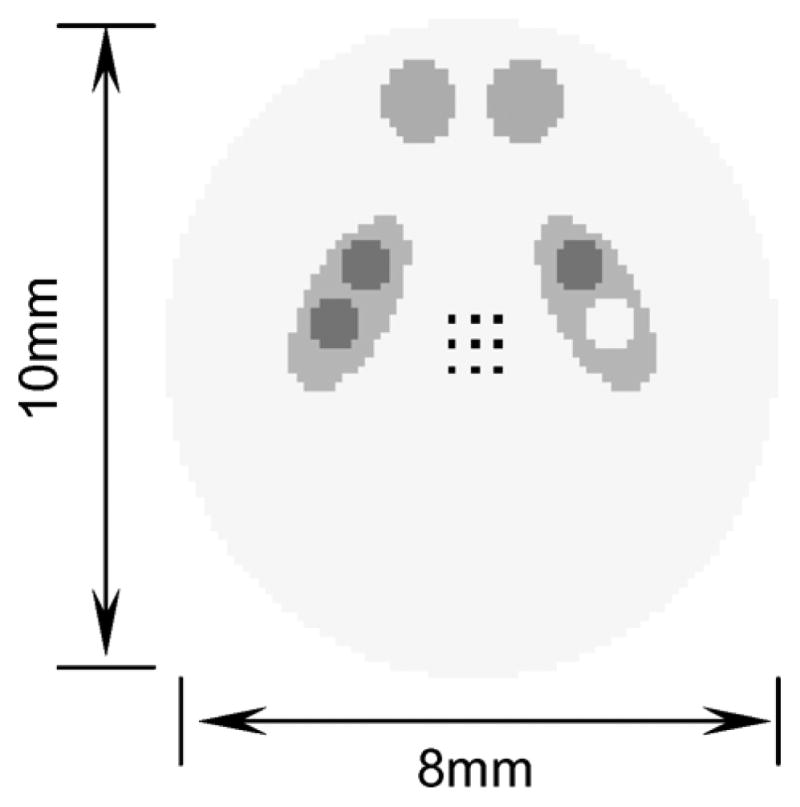
Cross sections of the resolution phantom. Nine control points were selected (as shown with black dots) for the calculation of the average resolution-variance tradeoffs.

III. Monte Carlo Results

A. Validation of MUCRB Calculation

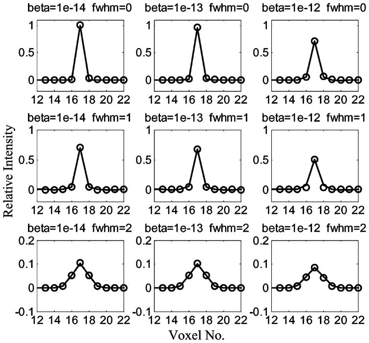
For linear Poisson problems, the vector MUCRB (23) can be achieved asymptotically with post-filtered penalized maximum likelihood (PF-PML) estimators. In this study, we compared the MUCRB with the empirical variance achieved with PF-PML estimators. To ensure the convergence of the PML estimators, 250 iterations were used in reconstructions. The source object contains a total activity of 100 μCi and the If one treats a pre-defined ROI as a big voxel, the bias on the estimated projection was acquired with an observation time of 1 hour. The empirical variance was obtained from 100 random realizations. In this comparison, a reasonably good agreement between the MUCRB and the empirical variance was demonstrated in Fig. 3. As discussed by several authors [29], [33], [40], the derivation of (M)UCRB does not include the non-negativity constraint that is enforced in PML estimators. For low count-rate situations and for PML estimators with a relatively small regularization, the minimum attainable variance predicted by MUCRB tends to be greater than that achievable with actual PM-PML estimators. This effect is also evident in Fig. 3. However, the difference between MUCRB and empirical variance of PF-PML estimator was kept below 7%, even with a small regularization factor (β ≤ 10⁻¹²). In this study, we also compared the LIRs predicted with (21) and those obtained from corresponding PF-PML estimators. An excellent agreement is demonstrated with the example shown in Fig. 4.

Fig. 3.

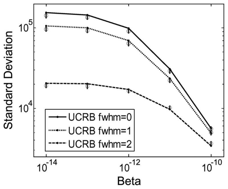
Comparing the MUCRB (curves) and the empirical variance value (circles with error bars) derived from Monte Carlo simulation. The detector pixel size was 350 μm. The standard deviation values were derived for the center pixel.

Fig. 4.

Local impulse functions for the center voxel. Solid lines: LIR of the optimum estimator that achieve the MUCRB. Circles: LIR obtained with actual PF-PML estimators. The regularization factor β and the FWHM of the 3-D Gaussian filter function are shown in the figure.

B. Monte Carlo Studies

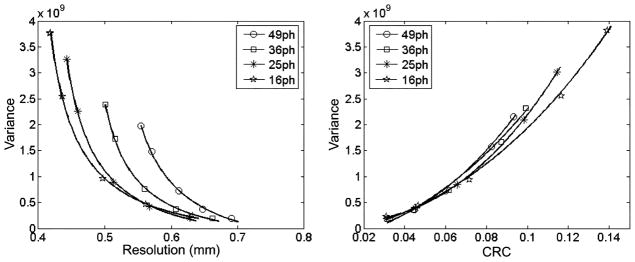
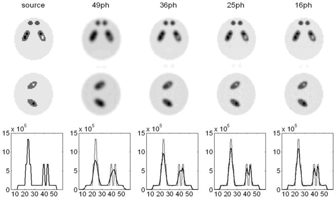
In this study, we compared the imaging performances of the SPECT system with different multiple-pinhole apertures. Each detector is 4.4 cm × 4.4 cm in size, with 350 μm pixels. The pinhole diameter was fixed to 200 μm. Four system configurations used are shown in Table II. For these configurations, the projections of the resolution phantom (Fig. 2) on the detector (4.4 cm × 4.4 cm) are compared in Fig. 5. The average resolution-variance and CRC-variance curves derived for different geometries are compared in Fig. 6. Reconstructed images of the brain phantom are compared in Fig. 7. These images were chosen to have similar average variances over the control points. Clearly, even without overlapping between projections through individual pinholes, the best imaging performance, judged by the resolution-variance tradeoffs and the visual appearance of reconstructed images, was achieved with the 16-pinhole aperture.

Fig. 5.

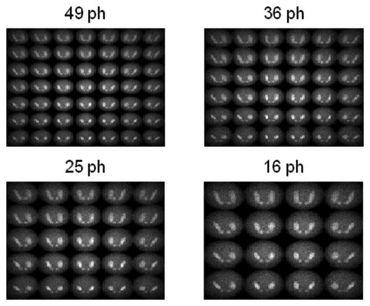
Projections of the resolution phantom on the 4.4 cm × 4.4 cm detector area.

Fig. 6.

Average resolution-variance (left) and CRC-variance (right) tradeoffs achieved with four system configurations as detailed in Table II.

Fig. 7.

Reconstructed images of the resolution phantom. The average variances over the nine control-points are similar for all four cases compared.

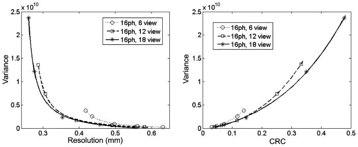
Since the proposed SPECT system will be installed inside an MRI scanner, the limited space available may prohibit the use of a rotating gantry. The motion of conductive material inside the magnet may also induce interference to MRI data acquisition. Therefore, it is desirable that SPECT system remains stationary during the SPECT image acquisition. However, the aperture ring may be designed to be relatively symmetric around the RF coil. A slight rotation of the aperture ring could provide a better angular sampling without disturbing the homogeneity of the main field. As another example for demonstrating the use of the MUCRB for system design, we evaluated the potential benefit of this rotation aperture scheme. During an imaging study, the aperture ring was rotated with one or two angular steps, with a fixed step-size of 2 degrees. A fixed imaging time of 1 hour was used. The resolution-variance curves corresponding to these imaging schemes are compared in Fig. 8. This result indicated that even a slight aperture rotation could lead to a much improved imaging performance. But for this given geometry, the benefit of multiple consecutive steps of rotation appears to be limited.

Fig. 8.

Average resolution-variance (left) and CRC-variance (right) tradeoffs achieved with the SPECT system and with the 16-pinhole aperture. Slight rotation of the aperture ring by a single step and by two consecutive steps of 2 degrees led to a significant improvement in resolution-variance tradeoffs.

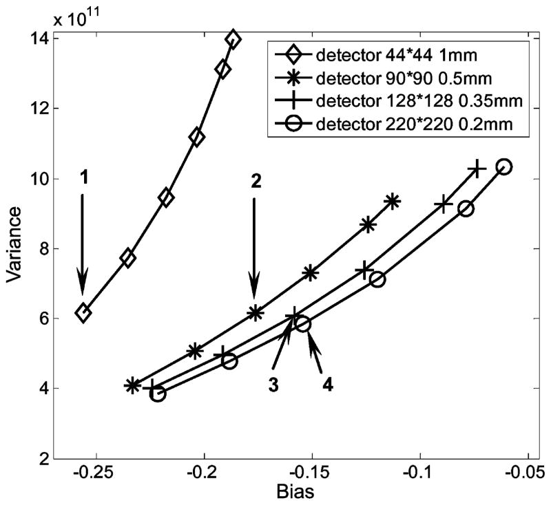
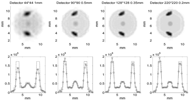
We have also used the proposed SPECT system to evaluate (30) and (31) for deriving the bias-variance curves for ROI quantitation. In this case, the 36 pinhole aperture was used and the detector pixel size was changing from 1 mm to 0.2 mm. A ROI was defined at the center of the FOV, which has a spherical volume of 1.6 mm in diameter. The bias and variance values derived using (30) and (31) were plotted against each other in Fig. 9. As demonstrated in this figure, improving detector resolution from 1 mm to 0.5 mm led to a significant improvement in ROI quantitation. Further improved resolution offered only a modest performance gain. These indications were confirmed by reconstructed images shown in Fig. 10. These images are corresponding to the four operation-points shown in Fig. 9. Once again, consistent results have been demonstrated between the analytically-derived system performance and the visual appearance of reconstructed images.

Fig. 9.

Bias-variance curves derived using (33). Reconstructed images corresponding to the four operation points are shown in Fig. 10.

Fig. 10.

Reconstructed images of the phantom with a hot blob at the center. These figures serve as a visual confirmation of the bias-variance tradeoff curves as shown in Fig. 6. The four columns are corresponding to the operation points highlighted in Fig. 9. The pixel sizes simulated and the total number of pixels in each detector are given on the top.

IV. Conclusions and Discussions

In this paper, we presented a generalized modified uniform Cramer-Rao bound. It gives the minimum attainable total (or average) variance by any estimator of an unknown deterministic vector parameter, given that the resultant mean gradient satisfies a certain constraint. The MUCRB can be used to evaluate the fundamental tradeoffs between resolution and image variance offered by a given system design. This method may serve as the basis for comparing different SPECT system and aperture designs. For linear Poisson model that commonly used to describe SPECT systems, the optimum resolution-variance tradeoffs predicted by MUCRB can be achieved asymptotically with post-filtered penalized likelihood reconstruction. This ensures that the system performance predicted is meaningful in routine practice.

In this study, the use of the MUCRB for evaluating system designs was demonstrated with a simulated stationary SPECT system. The tradeoffs between resolution and variance, as predicted by the MUCRB approach, are consistent with that obtained from reconstructed images. The evaluation of a single point on the tradeoff curve requires a computation load similar to that of a single image reconstruction. Given that the construction of a resolution-variance curve typically requires less than ten points in the resolution-variance space, the formulations derived allow quantitative system evaluations base on the statistical image quality with a reasonable computation time.

Fig. 1.

The proposed MRI-compatible SPECT system. Left penal: schematic of the SPECT system inside a MRI scanner. Right panel: dimensions of different components.

References

- 1.Peterson TE, Wilson DW, Barrett HH. Application of silicon strip detectors to small-animal imaging. Nucl Instrum Methods Phys Res A. 2003;A505:608–611. [Google Scholar]
- 2.Accorsi R, Curion AS, Frallicciardi P, Lanza RC, Lauria A, Mettivier G, Montesi MC, Russo P. Preliminary evaluation of the tomographic performance of the mediSPECT small animal imaging system. Nucl Instrum Methods Phys Res A. 2007;A571:415–418. [Google Scholar]
- 3.Beekman FJ, Vastenhouw B. Design and simulation of a high-resolution stationary SPECT system for small animals. Phys Med Biol. 2004;49:4579–4592. doi: 10.1088/0031-9155/49/19/009. [DOI] [PubMed] [Google Scholar]
- 4.Meng LJ, Clinthorne NH, Skinner S, Hay RV, Gross M. Design and feasibility study of a single photon emission microscope system for small animal I-125 imaging. IEEE Trans Nucl Sci. 2006 Jun;53(3):1168–1178. doi: 10.1109/TNS.2006.871405. [DOI] [PMC free article] [PubMed] [Google Scholar]
- 5.Miller BW, Barber HB, Barrett HH, Chen LY, Wilson DW. A low-cost approach to high-resolution, single-photon imaging using columnar scintillators and image intensifiers. Proc. IEEE NSS/MIC Conf. Rec; San Diego, CA. 2006. [Google Scholar]
- 6.Abbott MB, DeClerck YA, Chen Y-C, Furenlid L, Wilson D, Stevenson G, Whitaker M, Woolfenden J, Moats RA, Barrett HH. 100-micron resolution SPECT imaging of a neuroblastoma tumor model. presented at the 5th Annu. Society for Molecular Imaging Meeting; Sep. 2006. [Google Scholar]
- 7.Cao ZX, Bal G, Accorsi R, Acton PD. Optimal number of pinholes in multi-pinhole SPECT for mouse brain imaging—A simulation study. Phys Med Biol. 2005;50:4609–4624. doi: 10.1088/0031-9155/50/19/013. [DOI] [PubMed] [Google Scholar]
- 8.Meikle SR, Kench P, Weisenberger AG, Wojcik R, Smith MF, Majewski S, Eberl S, Fulton RR, Rosenfeld AB, Fulham MJ. A prototype coded aperture detector for small animal SPECT. IEEE Trans Nucl Sci. 2002 Oct;49(5):2167–2171. [Google Scholar]
- 9.Schramm N, Wirrwar A, Halling H. Development of a multi-pinhole detector for high-sensitivity SPECTimaging. Proc IEEE NSS/MIC Conf Rec. 2001 Nov;3:1585–1586. [Google Scholar]
- 10.Song TY, Choi Y, Chung YH, Jung JH, Choe YS, Lee KH, Kim SE, Kim BT. Optimization of pinhole collimator for small animal SPECT using Monte Carlo simulation. IEEE Trans Nucl Sci. 2003 Jun;50(3):327–332. [Google Scholar]
- 11.Beekman FJ, Vastenhouw B. Design and simulation of a high-resolution stationary SPECT system for small animals. Phys Med Biol. 2004;49:4579–4592. doi: 10.1088/0031-9155/49/19/009. [DOI] [PubMed] [Google Scholar]
- 12.van der Have F, Beekman FJ. Photon penetration and scatter in micro-pinhole imaging: A Monte Carlo investigation. Phys Med Biol. 2004;49:1369–1386. doi: 10.1088/0031-9155/49/8/001. [DOI] [PubMed] [Google Scholar]
- 13.Rentmeester MCM, van der Have F, Beekman FJ. Optimizing multi-pinhole SPECT geometries using an analytical model. Phys Med Biol. 2007;52:2567–2581. doi: 10.1088/0031-9155/52/9/016. [DOI] [PubMed] [Google Scholar]
- 14.Bal G, Zeng GL, Lewitt RM, Cao Z, Acton PD. Study of different pinhole configurations for small animal tumor imaging. Proc. IEEE NSS/MIC Conf. Rec; Oct. 2004; pp. 2214–2217. [Google Scholar]
- 15.Accorsi R, Gasparini F, Lanza RC. Optimal coded aperture patterns for improved SNR in nuclear medicine imaging. Nucl Instrum Methods Phys Res A. 2001;A474:273–284. [Google Scholar]
- 16.Barrett HH, Abbey CK, Clarkson E. Objective assessment of image quality. III. ROC metrics, ideal observers, and likelihood-generating functions. J Opt Soc Amer A Opt Image Sci. 1998;15:1520–1535. doi: 10.1364/josaa.15.001520. [DOI] [PubMed] [Google Scholar]
- 17.Barrett HH, Myers KJ, Devaney N, Dainty C. Objective assessment of image quality. IV. Application to adaptive optics. J Opt Soc Amer A Opt Image Sci. 2006;23:3080–3105. doi: 10.1364/josaa.23.003080. [DOI] [PMC free article] [PubMed] [Google Scholar]
- 18.Rolland JP, Barrett HH. Effect of random background inhomogeneity on observer detection performance. J Opt Soc Amer A Opt Image Sci. 1992;9:649–658. doi: 10.1364/josaa.9.000649. [DOI] [PubMed] [Google Scholar]
- 19.Khurd P, Gindi G. Decision strategies that maximize the area under the LROC curve. IEEE Trans Med Imag. 2005;24:1626–1636. doi: 10.1109/TMI.2005.859210. [DOI] [PubMed] [Google Scholar]
- 20.Gifford HC, King MA, Pretorius PH, Wells RG. A comparison of human and model observers in multislice LROC studies. IEEE Trans Med Imag. 2005;24:160–169. doi: 10.1109/tmi.2004.839362. [DOI] [PubMed] [Google Scholar]
- 21.Gilland KL, Tsui BMW, Qi YJ, Gullberg GT. Comparison of channelized hotelling and human observers in determining optimum OS-EM reconstruction parameters for myocardial SPECT. IEEE Trans Nucl Sci. 2006 Jun;53(3):1200–1204. [Google Scholar]
- 22.Yendiki A, Fessler JA. Analysis of observer performance in known-location tasks for tomographic image reconstruction. IEEE Trans Med Imag. 2006;25:28–41. doi: 10.1109/TMI.2005.859714. [DOI] [PubMed] [Google Scholar]
- 23.Barrett HH, Myers K. Foundations of Image Science. New York: Wiley; 2004. [Google Scholar]
- 24.Van Trees HL. Detection, Estimation and Modulation Theory. New York: Wiley; 1968. [Google Scholar]
- 25.Hero AO, Fessler JA, Usman M. Exploring estimator bias-variance tradeoffs using the uniform CR bound. IEEE Trans Signal Process. 1996;44:2026–2041. [Google Scholar]
- 26.Hero A, Fessler JA. A recursive algorithm for computing Cramer-Rao-type bounds on estimator covariance. IEEE Trans Inf Theory. 1994;40:1205–1210. [Google Scholar]
- 27.Hua CH, Clinthorne NH, Wilderman SJ, LeBlanc JW, Rogers WL. Quantitative evaluation of information loss for Compton cameras. IEEE Trans Nucl Sci. 1999 Jun;46(3):587–593. [Google Scholar]
- 28.Kragh T. PhD dissertation. Univ. Michigan; Ann Arbor: 2002. Application of Uniform Cramer-Rao Bounds. [Google Scholar]
- 29.Meng LJ, Clinthorne NH. A modified uniform Cramer-Rao bound for multiple pinhole aperture design. IEEE Trans Med Imag. 2004;23:896–902. doi: 10.1109/TMI.2004.828356. [DOI] [PMC free article] [PubMed] [Google Scholar]
- 30.Fessler JA, Rogers WL. Spatial resolution properties of penalized-likelihood image reconstruction: Space-invariant tomographs. IEEE Trans Image Process. 1996;5:1346–1358. doi: 10.1109/83.535846. [DOI] [PubMed] [Google Scholar]
- 31.Meng LJ, Clinthorne NH, Skinner S, Hay RV, Gross M. Design and feasibility study of a single photon emission microscope system for small animal I-125 imaging. IEEE Trans Nucl Sci. 2006 Jun;53(3):1168–1178. doi: 10.1109/TNS.2006.871405. [DOI] [PMC free article] [PubMed] [Google Scholar]
- 32.Eldar YC. Minimum variance in biased estimation: Bounds and asymptotically optimal estimators. IEEE Trans Signal Process. 2004;52:1915–1930. [Google Scholar]
- 33.Fessler JA. Mean and variance of implicitly defined biased estimators (such as penalized maximum likelihood): Applications to tomography. IEEE Trans Image Process. 1996;5:493–506. doi: 10.1109/83.491322. [DOI] [PubMed] [Google Scholar]
- 34.Qi JY, Leahy RM. A theoretical study of the contrast recovery and variance of MAP reconstructions from PET data. IEEE Trans Med Imag. 1999;18:293–305. doi: 10.1109/42.768839. [DOI] [PubMed] [Google Scholar]
- 35.Meng LJ, Wehe DK. Feasibility study of using hybrid collimation for nuclear environmental imaging. IEEE Trans Nucl Sci. 2003 Aug;50(4):1103–1110. doi: 10.1109/TNS.2003.815135. [DOI] [PMC free article] [PubMed] [Google Scholar]
- 36.Qi JY, Huesman RH. Theoretical study of penalized-likelihood image reconstruction for region of interest quantification. IEEE Trans Med Imag. 2006;25:640–648. doi: 10.1109/TMI.2006.873223. [DOI] [PubMed] [Google Scholar]
- 37.Meng LJ, Tan JW, Fu G. Design study of an MRI compatible ultra-high resolution SPECT for in vivo mice brain imaging. Proc IEEE NSS/MIC Conf Rec. 2007;4:2956–2960. [Google Scholar]
- 38.Shepp LA, Vardi Y. Maximum likelihood reconstruction in positron emission tomography. IEEE Trans Med Imag. 1982;1:113–122. doi: 10.1109/TMI.1982.4307558. [DOI] [PubMed] [Google Scholar]
- 39.Qi JY, Leahy RM. Resolution and noise properties of MAP reconstruction for fully 3-D PET. IEEE Trans Med Imag. 2000;19:493–506. doi: 10.1109/42.870259. [DOI] [PubMed] [Google Scholar]
- 40.Numerical Recipes in C. ch 7. Cambridge, U.K: Cambridge Univ. Press; 1997. p. 0-521-43720-2. [Google Scholar]