Abstract
A fault diagnosis approach based on multi-sensor data fusion is a promising tool to deal with complicated damage detection problems of mechanical systems. Nevertheless, this approach suffers from two challenges, which are (1) the feature extraction from various types of sensory data and (2) the selection of a suitable fusion level. It is usually difficult to choose an optimal feature or fusion level for a specific fault diagnosis task, and extensive domain expertise and human labor are also highly required during these selections. To address these two challenges, we propose an adaptive multi-sensor data fusion method based on deep convolutional neural networks (DCNN) for fault diagnosis. The proposed method can learn features from raw data and optimize a combination of different fusion levels adaptively to satisfy the requirements of any fault diagnosis task. The proposed method is tested through a planetary gearbox test rig. Handcraft features, manual-selected fusion levels, single sensory data, and two traditional intelligent models, back-propagation neural networks (BPNN) and a support vector machine (SVM), are used as comparisons in the experiment. The results demonstrate that the proposed method is able to detect the conditions of the planetary gearbox effectively with the best diagnosis accuracy among all comparative methods in the experiment.
Keywords: fault diagnosis, multi-sensor data fusion, deep convolutional neural networks, feature learning, planetary gearbox
1. Introduction
The planetary gearbox is a key component in mechanical transmission systems and has been widely used in wind turbines, helicopters and other heavy machineries [1]. The wide range of gear ratios, small room in power transmission line, and high transmission efficiency are the most significant advantages of planetary gearboxes [2]. Planetary gearboxes generally operate in tough working environments, which makes them suffer from a variety of failures and damages [1,3] causing unwanted downtime, economic losses, and even human casualties [4]. Therefore, the fault diagnosis of planetary gearboxes is necessary to guarantee a safe and efficient operation of mechanical transmission systems.
Health conditions of planetary gearboxes can be reflected by various kinds of measurements, including vibration signal, acoustic signal, driven motor current, shaft speed, oil debris, etc. Different measurements have different drawbacks and are sensitive to different types of damage modes or operation conditions. Thus, combining and analyzing these measurements together should be an appropriate approach to detect various types of faults of complex systems. This approach, named multi-sensor data fusion, can achieve more accurate and reliable result than approaches with a single sensor [5,6,7].
Nevertheless, multi-sensor data fusion for fault diagnosis suffers from two challenging problems [6]. (1) One is the feature extraction of multi-sensory data. Generally, conventional fault diagnosis includes three steps [8]: signal acquisition, feature extraction, and fault classification. In the feature extraction step, fault sensitive features are extracted and selected from raw data through signal processing technologies and data analysis strategies, such as Fourier spectral analysis, wavelet transformation (WT), and principal component analysis (PCA). However, the multiple types of sensory data of multi-sensor data fusion may cause a number of issues that make the feature extraction with multi-sensor much more difficult than with a single sensor. These issues [6,7] include more imprecision and uncertainties in measurements, various noises, more conflicting or correlating data, higher data dimensions, etc. Extracting features from these kinds of data will be a very challenging and cruel task. At the same time, multiple types of sensory data also increases the difficulties and consumes much time to choose an optimal handcraft feature or manual feature extraction method, even though to date, the optimal handcraft feature or feature extraction method for a specific type of sensory data still remains unanswered [8,9]; (2) The other challenge of the multi-sensor data fusion is the selection of different fusion levels. Similarly, different fusion levels have their own advantages and disadvantages, and the suitable one for different fault diagnosis tasks is usually different [5]. Selecting an optimal fusion level for a specific fault diagnosis task always requires domain expertise, prior knowledge, and human labor.
Deep neural networks (DNN), also known as deep learning, have been attracting increasing attention from researchers from various fields in recent years [10,11,12]. The key advantage of DNN is the feature learning ability [11], which can automatically discover an intricate structure and learn useful features from raw data layer by layer. A number of studies [11,12,13] have shown that DNN can fuse input raw data and extract basic information from it in its lower layers, fuse the basic information into higher representation information and decisions in its middle layers, and further fuse these decisions and information in its higher layers to form the final classification result. It can be seen that DNN itself is a fusion structure [11,13], which fuses the feature extraction, feature selection, data-level fusion, feature-level fusion, decision-level fusion, and classification into one single learning body. For this reason, a DNN-based low level fusion, e.g., data-level fusion, can not only learn features from fused raw data automatically, but also fuse these data, features and decisions adaptively through its deep-layered structure. DNN might be an ideal model to fuse multi-sensory data and detect faults of a mechanical system. However, although some applications [14,15,16,17,18] of DNN in feature learning and fault diagnosis with a single sensor have been found in recent years, no study, to the best of our knowledge, has investigated the effectiveness of DNN-based feature learning and the adaptive level fusion method for fault diagnosis. It is attractive and meaningful to investigate this adaptive fusion method, which can learn features from raw data automatically, and select and combine fusion levels adaptively.
Deep convolutional neural networks (DCNNs), as one of the main types of DNN models, have been successfully used in mechanical fault diagnosis with automatic feature learning from single sensory data [9,14,19,20]. Benefitting from several unique structures, DCNN can achieve better results with less training time than standard neural networks. Firstly, DCNN has a large set of filter kernels in convolutional layers, which can capture representative information and patterns from raw data. Stacking these convolutional layers can further fuse information and build complex patterns; Secondly, DCNN is an unfully-connected network, where each filter shares the same weights. This structure can reduce both the training time and complication of the model. In addition, the pooling layer of DCNN further reduces the revolution of the input data as well as the training time, and improves the robustness of the extracted patterns (a detailed introduction to the DCNN model is presented in Section 2). Thus, DCNN should have great potential in processing the multi-sensory data of a mechanical system, which usually contains rich information in the raw data and is sensitive to training time as well as model size.
Aiming to address the two problems of multi-sensor data fusion mentioned above, this paper proposes an adaptive data fusion method based on DCNN and applies it to detect the health conditions of a planetary gearbox. Different from conventional methods, the proposed method is able to (1) extract features from raw data automatically and (2) optimize a combination of different fusion levels adaptively for any specific fault diagnosis task with less dependence on expert knowledge or human labor.
The rest of the paper is organized as follows. In Section 2, the typical architecture of DCNN and an adaptive training method are briefly described. Section 3 illustrates the procedures of the proposed method, the design of the DCNN model, and several comparative methods introduced to further analyze the performance of the proposed method. In Section 4, an experimental system of a planetary gearbox test rig is used to validate the effectiveness of the proposed method. Finally, the conclusions are drawn in Section 5.
2. Deep Convolutional Neural Networks
2.1. Architecture of Deep Convolutional Neural Networks
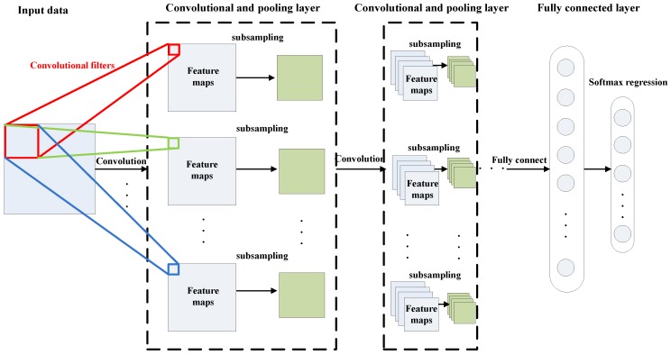
DCNN is a type of DNN model inspired by visual system structure [11,21], and it has become the dominant approach for almost all recognition and detection tasks in image and speech analysis [22,23,24]. DCNN contains three kinds of layers [25], which are the convolutional layer, pooling layer, and fully-connected layer. As shown in Figure 1, the first several layers of a typical DCNN usually consist of a combination of two types of layers—convolutional layers, followed by pooling layers—and the last layer is a fully-connected layer. In the following part, we will describe these three kinds of layers in more detail.
Figure 1.
A typical architecture of deep convolutional neural network (DCNN).
The convolutional layer is composed of a number of two-dimensional (2D) filters with weighted parameters. These filters convolute with input data and obtain an output, named as feature maps. Each filter shares the same weighted parameters for all the patches of the input data to reduce the training time and complication of the model, which is different from a traditional neural network with different weighted parameters for different patches of the input data. Suppose the input of the convolutional layer is , which belongs to , and A and B are the dimensions of the input data. Then the output of the convolutional layer can be calculated as follows [26]:
| (1) |
where is the cn-th output of the convolutional layer, and the output number is CN, which is also equal to the filter number; is an operator of convolution; represents the input data of cc-th channel of previous layer − 1, and the channel number is CC; is the weight of cn-th filter of the current layer l; the width and height of the filter are CW and CH, respectively; the cn-th bias is denoted with ; is an activation function, typically hyperbolic tangent or sigmoid function.
The pooling layer is a sub-sampling layer, which reduces the revolution of the input data and improves the robustness of learned features. A pooling layer generally follows a convolutional layer with a max pooling method and it outputs only the maximum of each sub-sampling patch of the feature maps to subsample the feature maps from the previous convolutional layer. The output can be described as follows [26]:
| (2) |
where is the cn-th output of the pooling layer, and the output number is CN; S is the pooling block size. This function will sum over each distinct S pooling block in the input data so that the output will become S times smaller along both spatial dimensions.
The fully-connected layer is the last layer of the DCNN model. It follows several combinations of the convolutional layers and the pooling layers, and classifies the higher-level information from the previous layers. A fully-connected layer is similar to a traditional multilayer neural network with a hidden layer and a classification layer, typically using a softmax regression. Assuming that the task is a K-label problem, the output of the softmax regression can be calculated as follows:
| (3) |
where are the parameters of the model, and is the final result of the DCNN.
2.2. Training Method
It can be seen from the previous description that , , and are the learnable parameters and will be optimized through model training with gradient decent algorithms. Since a gradient decent algorithm is easily trapped into local optima, we introduce several enhancement methods, including stochastic gradient decent (SGD), cross-validation, and adaptive learning rate, to solve this problem. SGD updates gradient [27] based on a few training data instead of the entire training set. This approach not only increases the training speed, but also improves the training reliability. Cross-validation selects a validation set from training data to test the performance of the parameters of the model to avoid overfitting. Since a global constant learning rate easily causes either a slow convergence with a lower learning rate or a serious fluctuation of the convergence with a higher learning rate, an adaptive learning rate is employed. The adaptive learning rate has a high rate at first and decreases with the increase of the training epochs adaptively to obtain a fast and reliable convergence result.
3. Adaptive Multi-Sensor Data Fusion Method Based on DCNN for Fault Diagnosis
3.1. Procedure of the Proposed Method
An adaptive multi-sensor data fusion method based on DCNN is presented to learn features from raw data automatically and combine fusion levels adaptively to detect faults of a planetary gearbox. Through its deep-layered structure, DCNN can fuse input data and extract basic features in the lower layers, fuse basic features into high level features and decisions in the middle layers, and further fuse these features and decisions in the higher layers to obtain the final diagnosis result.
Figure 2 displays the flowchart of the proposed method: (1) four types of signals, including vibration signal [3,28,29], acoustic signal [4,30], current signal [31,32,33], and instantaneous angular speed (IAS) signal [34,35], are selected according to published studies and acquired from a planetary gearbox; (2) data preprocessing is applied to standardize each signal and divide them into segments; (3) each of the four segments of the four signal types are combined together simply as one data sample to form the data-level fused input data of the DCNN model; (4) DCNN is trained and tested with these fused input data, and its output will be the diagnosis result of the planetary gearbox. The testing accuracy of the output result is used to evaluate the effectiveness of the proposed method. It should be noted that although we use a data-level fusion in the third step, data is fused again in the starting layers of the DCNN model to further optimize the data structure. The DCNN implicitly contains data-level fusion, feature-level fusion, and decision-level fusion through the deep-layered structure and it optimizes a combination of these fusion levels adaptively according to the characteristic of the data itself.
Figure 2.
Flowchart of the proposed method.
3.2. Model Design of DCNN
The model of DCNN is adjusted to satisfy the characteristics of mechanical fault diagnosis. Although most applications of DCNN in image recognition chose a 2D convolutional structure [11,22,36], and some researchers [20,37] also used the same way to diagnose mechanical faults, we select a one-dimensional (1D) convolutional structure with a 1D filter bank as the kernel of the DCNN model. In our opinion, the main reason behind the applications of the 2D convolutional structure of DCNN in image analysis lies in the natural 2D space correlation in images. However, most of the measurement data for mechanical fault diagnosis only correlate with time, which is a 1D parameter. Thus, 1D convolutional structure should be an appropriate choice for a DCNN-based fault diagnosis problem. In addition, we choose a larger filter size than conventional ones used in image recognition. While a larger size of the filter may be more expensive in terms of computation, a larger filter can capture more information between the data farther away from each other [38], which may be the features in the frequency domain.
In spite of the many benefits of the deep-layered structure of DCNN, a “deep” structure also means complicated hyper-parameters as well as various choices of architectures, which increases the difficulty to build an appropriate and efficient model. Although there are several researches [39,40] about the automatic optimization of parameters of DCNN, the optimized process is usually time-consuming and easily converges into a local optimum due to the large number of parameters of DCNN. Thus, we build the DCNN model initially based on a few general design principles [38,41]. Then several configurations of the network are tested using the experimental data, and the one with best performance is selected as the setting of the final model.
3.3. Comparative Methods
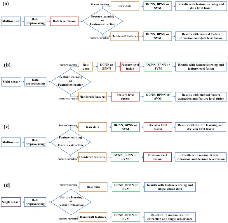
Several comparative methods are employed to further test and confirm the performance of the proposed method. The flowcharts of comparative methods are shown in Figure 3.
Figure 3.
Flowcharts of comparative methods: (a) Data-level fusion methods; (b) Feature-level fusion methods; (c) Decision-level fusion methods; and (d) Methods with single sensory data.
To evaluate the ability of learning features from the raw data of the proposed method, manual feature extraction is used as a replacement and comparison of the feature learning in each comparative method. Eight time-domain features and several frequency-domain features are extracted. Root mean square (RMS), kurtosis, crest factor, skewness, mean, minimum, maximum, and variance are chosen as the handcraft features in the time domain [34,37,42]. The characteristic frequencies of the planetary gearbox [1], including the rotating frequencies of the sun gear, planetary gear and the carrier, the pass frequency of the planetary gear and the meshing frequency of the planetary gearbox, are selected as the handcraft features in the frequency domain as well as their ten sidebands for all types of the sensor signals [34,43,44] except for the current signal. For the current signal, the line frequency and its sidebands [45] generated by the modulation of the characteristic frequencies of the planetary gearbox are chosen as its frequency-domain features. In addition, the fast Fourier-transform (FFT) energy of each sample, which is obtained by splitting the frequency spectrum of each sample into 32 average bands and calculating the RMS of each band [46], is also added into the handcraft features in the frequency domain. While all the domain features are processed together as the “handcraft features”, the “time-domain features” and “frequency-domain features” are also tested respectively to reflect more information about the sensitivity of the data. The comparison between the learning features from raw data and the handcraft features is marked in orange in Figure 3.
As a comparison of the DCNN model of the proposed method, two intelligent models, back-propagation neural networks (BPNN) and support vector machine (SVM), are introduced as replacements of DCNN in each comparative method. BPNN is built into a three-layer model with sigmoid activation functions. SVM uses Gaussian radial basis function (RBF) as the kernel function and the grid search method to optimize the parameters of the kernel. The three comparative models, DCNN, BPNN, and SVM, are marked in green in Figure 3.
For testing the performance of the different fusion levels, manual-selected feature-level fusion and decision-level fusion are explored and compared with the data-level fusion of the proposed method. For feature-level fusion with feature learning from raw data, only DCNN and BPNN are applied to learn features from the raw data of each sensor, respectively. The outputs of the second-last layers of DCNN are extracted as the learned features of each sensory data. Then, all the learned features from the four types of sensors are combined together as the feature-level fused features and used as the input of another DCNN for classification. In the same way, the outputs of the second-last layers of BPNN are extracted and fused. Then, the fused features are used as the input of both BPNN and SVM for classification. The comparison of different fusion levels is marked in red in Figure 3.
As a comparison of the multi-sensory input data of the proposed method, fault diagnosis with single sensory data is also applied to evaluate the effectiveness of the proposed method, which is marked in purple and shown in Figure 3d.
4. Experiment and Discussion
4.1. Experiment Setup
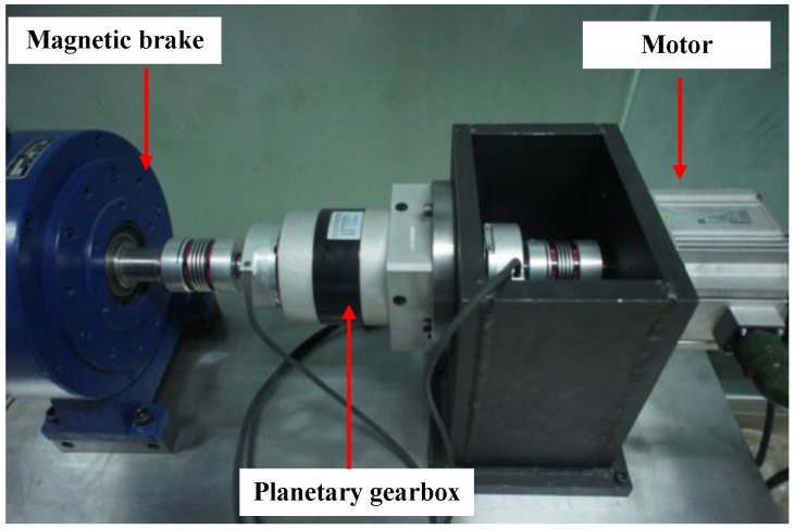
An experimental system of a planetary gearbox test rig is established to evaluate the effectiveness of the proposed method. As shown in Figure 4, it consists of a one-stage planetary gearbox, a driven motor and a magnetic brake. The planetary gearbox contains one 20-tooth sun gear and three 31-tooth planetary gears, and transmits torque from the sun gear to the planetary carrier of the planetary gears with a standstill ring gear.
Figure 4.
Planetary gearbox test rig.
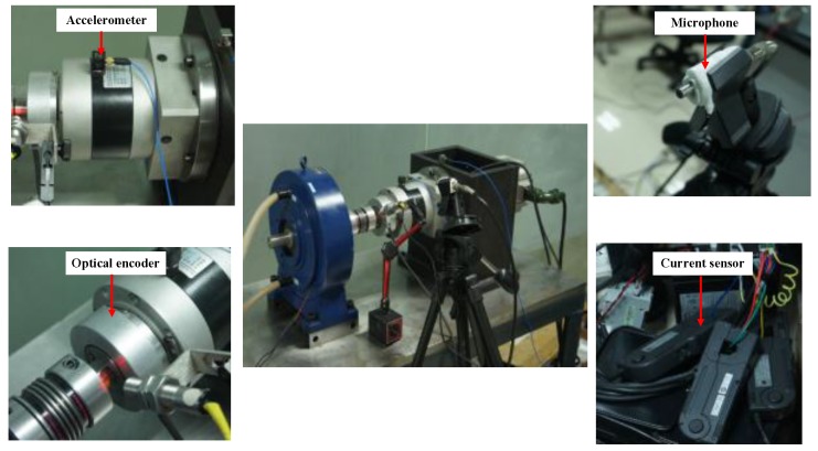
Figure 5 presents the four types of sensors employed in the experiment, including an accelerometer, microphone, current sensor, and optical encoder. Vibration signal, acoustic signal, and motor current signal are measured by their corresponding sensors and acquired through a data acquisition box with a sampling frequency of 20 kHz and data length of 320 k points. The IAS of the output shaft is calculated based on counting the number of high resolution pulses of the encoder [47]; and down-sampling, using the data acquisition box with the same sampling frequency and data length as the other three signals.
Figure 5.
Four types of sensors and their installations.
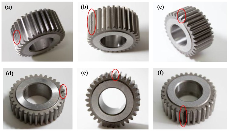
Seven health conditions of the planetary gearbox are tested, including normal, pitting tooth, chaffing tooth, chipped tooth, root crack tooth, slight worn tooth, and worn tooth. As shown in Figure 6, all the faults occurred in the planetary gears. In each experiment, only one planetary gear with one kind of health condition is examined, and all the other gears are normal. Experiments are conducted under three motor speeds (600 rpm, 1200 rpm and 1800 rpm) and a load-free condition. The detailed description for the datasets and pattern labels of the experiment is shown in Table 1.
Figure 6.
Faulty planetary gears: (a) Pitting tooth; (b) Chaffing tooth; (c) Chipped tooth; (d) Root crack tooth; (e) Slight worn tooth; and (f) Worn tooth.
Table 1.
Description of the pattern labels of planetary gearbox data.
| Pattern Label | Gearbox Condition | Input Speed (rpm) | Load |
|---|---|---|---|
| 1 | Normal | 600, 1200 and 1800 | Zero |
| 2 | Pitting tooth | 600, 1200 and 1800 | Zero |
| 3 | Chaffing tooth | 600, 1200 and 1800 | Zero |
| 4 | Chipped tooth | 600, 1200 and 1800 | Zero |
| 5 | Root cracked tooth | 600, 1200 and 1800 | Zero |
| 6 | Slight worn tooth | 600, 1200 and 1800 | Zero |
| 7 | Worn tooth | 600, 1200 and 1800 | Zero |
4.2. Data Processing
The acquired vibration signal, acoustic signal, current signal, and IAS signal are preprocessed following the steps in Section 3.1. For the proposed method, the collected signals are standardized and divided into segments at first. A total of 1024 points are selected as a segment, so each type of signal will contain 312 segments for each health condition under one motor speed and 6552 segments in total for seven health conditions under three motor speeds. Next, each of the four segments of the four signal types are combined together as one data sample to form the input vectors of the DCNN model. In this way, each data sample will be a 4096-dimensional vector (four times the size of segments), and there will be 6552 data samples in total. A total of 40% of the 6552 data samples are selected randomly as the training data set, 10% are used as the validation set, and the remaining 50% are selected as the testing data set. Eight trails are carried out to avoid particularity and contingency of the diagnosis result. The average testing accuracy of the eight trails is calculated as the final result.
4.3. Model Design
The model of the DCNN is developed using the principles described in Section 3.2. For different input data, different model settings are tested, and the one with the best performance among all the tested settings is selected to process this input data. The model setting of the proposed method is displayed in Table 2, which consists of three convolutional layers, two pooling layers, and a fully-connected layer with softmax regression. The convolutional layer corresponds to Equation (1), the pooling layer to Equation (2) and the fully-connected layer to Equation (3). The DCNN model is developed based on C++.
Table 2.
Variables of parameters and structures of the deep convolutional neural networks.
| Layer | Type | Variables and Dimensions | Training Parameters |
|---|---|---|---|
| 1 | Convolution | CW = 65; CH = 1; CC = 1; CN = 10; B = 10 | SGD minibatch size = 20 |
| 2 | Pooling | S = 2 | Initial learning rate = 0.05 |
| 3 | Convolution | CW = 65; CH = 1; CC = 10; CN = 15; B = 15 | Decrease of learning rate after each ten epochs = 20% |
| 4 | Pooling | S = 2 | Momentum = 0.5 |
| 5 | Convolution | CW = 976; CH = 1; CC = 15; CN = 30; B = 30 | Weight decay = 0.04 |
| 6 | Hidden layer | Relu activation function | Max epochs = 200 |
| 7 | Softmax | 7 outputs | Testing sample rate = 50% |
SDG = stochastic gradient decent; CW = filter width; CH = filter height; CC = filter channel; CN = number of filter in the bank; B = bias; S = sub-sampling rate; No overlapping of convolutional window and no padding.
4.4. Experimental Results
4.4.1. Results of Single Sensory Data
Following the flowchart shown in Figure 3d in Section 3.3, methods with three intelligent models, feature learning and manual feature extraction methods, and four types of single sensor data are tested in the experiment. The results are displayed in Table 3.
Table 3.
Average testing accuracy of comparative methods with single sensory data.
| Sensory Data | Model | Feature Learning from Raw Data | Manual Feature Extraction | ||
|---|---|---|---|---|---|
| Time-Domain Features | Frequency-Domain Features | Handcraft Features | |||
| Vibration signal | DCNN | 81.45% | 55.84% | 70.74% | 73.64% |
| BPNN | 42.56% | 55.62% | 69.03% | 72.36% | |
| SVM | 45.11% | 56.35% | 72.23% | 73.86% | |
| Acoustic signal | DCNN | 66.23% | 31.42% | 76.45% | 76.02% |
| BPNN | 19.80% | 35.89% | 76.04% | 75.79% | |
| SVM | 26.54% | 33.62% | 77.36% | 76.32% | |
| Current signal | DCNN | 85.68% | 60.73% | 61.45% | 76.85% |
| BPNN | 52.36% | 60.47% | 61.21% | 76.43% | |
| SVM | 51.64% | 63.74% | 63.53% | 78.76% | |
| Instantaneous angular speed (IAS) signal | DCNN | 90.23% | 75.34% | 84.42% | 88.34% |
| BPNN | 51.37% | 75.36% | 85.22% | 89.82% | |
| SVM | 48.22% | 75.68% | 85.65% | 89.85% | |
DCNN = deep convolutional neural network; BPNN = back-propagation neural networks; SVM = support vector machine.
4.4.2. Results of Multi-Sensory Data
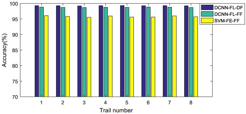
Following the flowcharts shown in Figure 3a–c in Section 3.3, methods with three fusion levels, three intelligent models, two feature extraction methods, and multi-sensory data are tested in the experiment. The results are displayed in Table 4, in which the result of the proposed method is marked in bold. Figure 7 presents the testing results of the eight trails of the top three methods, which are the proposed method, the DCNN model with feature learning and feature-level fusion, and the SVM model with handcraft features and feature-level fusion.
Table 4.
Average testing accuracy of comparative methods with multi-sensory data.
| Fusion Level | Model | Feature Learning from Raw Data | Manual Feature Extraction | ||
|---|---|---|---|---|---|
| Time-Domain Features | Frequency-Domain Features | Handcraft Features | |||
| Data-level fusion | DCNN | 99.28% | 66.08% | 87.63% | 90.23% |
| BPNN | 53.28% | 65.95% | 87.89% | 91.22% | |
| SVM | 51.62% | 67.32% | 87.28% | 90.67% | |
| Feature-level fusion | DCNN | 98.75% | 86.35% | 92.34% | 94.08% |
| BPNN | 64.74% | 86.81% | 92.15% | 94.04% | |
| SVM | 56.27% | 86.74% | 94.62% | 95.80% | |
| Decision-level fusion | DCNN | 93.65% | 84.65% | 90.23% | 92.19% |
| BPNN | 77.62% | 84.47% | 91.19% | 93.42% | |
| SVM | 76.17% | 86.32% | 90.98% | 93.44% | |
Figure 7.
Testing accuracy of eight trials of the top three methods (the proposed method, the DCNN model with feature learning and feature-level fusion, and the SVM model with handcraft features and feature-level fusion). FL = feature learning; FE = manual feature extraction; DF = data-level fusion; FF = feature-level fusion.
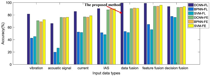
Finally, the average testing accuracies of all the comparative methods in the experiment are shown together in Figure 8 for a clearer comparison between each other.
Figure 8.
Testing accuracy of all the comparative methods.
4.5. Principal Component Analysis of the Experimental Data and Learned Features
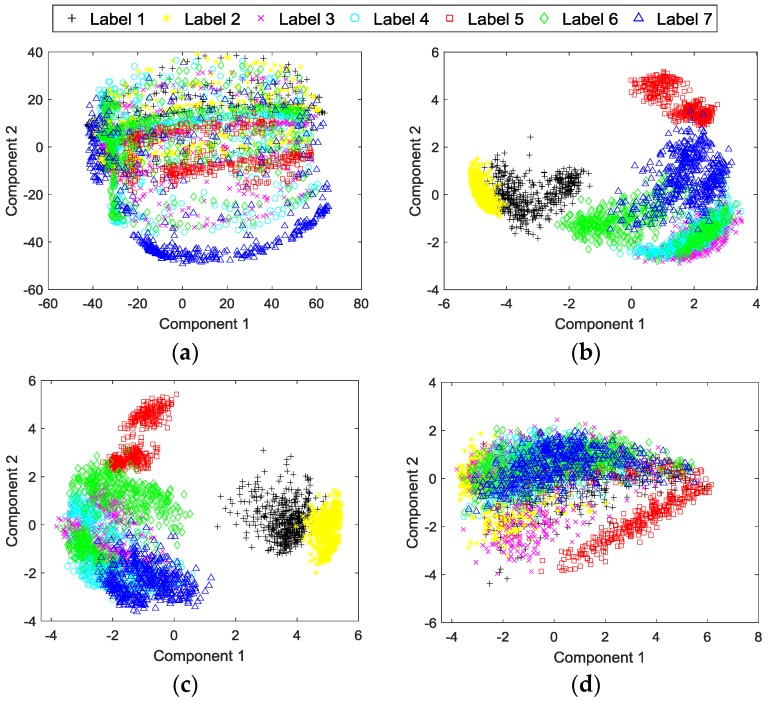
PCA is employed to analyze and visualize the learned features of the proposed method. As shown in Figure 9, the labels 1 to 7 correspond to the seven conditions of the planetary gearbox described in Table 1, and the first two principal components (PCs) are obtained by PCA to represent the useful information hidden in the data. Figure 9a shows the result of the input data of the testing dataset of the proposed method along the first two PCs. Figure 9b illustrates the result of the learned features with adaptive fusion levels of the proposed method for testing the dataset, which are extracted from the output of the second-last layer of the DCNN. For comparison, the results of feature-level fused features learned through DCNN and feature-level fused handcraft features along the first two PCs are shown in Figure 9c,d, respectively. It should be noted that we only display the first two PCs of the data for a clearer visualization, which means that there may be overlaps between some categories and many of them can be divided into higher PCs.
Figure 9.
Principal component analysis (PCA) of the experimental data and learned features: (a) Data-level fused input data of the proposed method; (b) Features of the proposed method; (c) Feature-level fused features learned through DCNN; and (d) Feature-level fused handcraft features.
4.6. Discussion
The experimental results show that the proposed method is able to diagnose the faults of the planetary gearbox test rig effectively, yielding the best testing accuracy in the experiment. It can be seen from Table 4 and Figure 8 that the proposed method achieves the best testing accuracy 99.28% among all the comparative methods. We think that this result is significantly correlated with the deep architecture of the DCNN model of the proposed method. DCNN can fuse input data and learn basic features from it in its lower layers, fuse basic features into higher level features or decisions in its middle layers, and further fuse these features and decisions to obtain the final result in its higher layers. Although there is a data-level fusion before DCNN in the proposed method, DCNN still actually fuses the data again in its starting layers to further optimize the data structure. Optimized features and combinations of different level fusions are formed through this deep-layered model, which provides a better result than with manually selected features or fusion levels.
The ability of automatic feature learning of the DCNN model with multi-sensory data is proven through the experiment. It can obviously be seen from Figure 8 that both the proposed method and the feature-level fusion method with feature learning through DCNN obtain a better result, 99.28% and 98.75%, than any other comparative methods with handcraft features or feature learning through BPNN. This result proves that the feature learning through DCNN with multi-sensory data can improve the performance of the multi-sensor data fusion method for fault diagnosis. In addition, the result also implies that the proposed method with adaptive fusion-level selection can achieve a better result 99.28% than the result 98.75% of the method with manual-selected feature-level fusion, which is the only difference between these two methods.
However, the method with automatic feature learning of DCNN from the raw signal of a single sensor cannot achieve a better result than methods with handcraft features. Table 3 displays the diagnosis results using signals from a single sensor. Only with a vibration signal and current signal, can the DCNN-based feature learning method achieve better results than conventional methods with handcraft features. By contrast, the results of the DCNN-based feature learning method with an acoustic signal and IAS signal are worse than that of conventional methods. This implies that the DCNN-based method with learned features from single sensory data cannot provide stable improvements for all kinds of sensory data. We think that the performance of the DCNN-based feature learning is influenced by the characteristics of the input data. As can be seen from the results shown in Table 3, the performance of feature learning has a stronger positive correlation with the performance of time-domain features than frequency-domain features, which infers that the DCNN-based feature learning from a raw signal may be more sensitive to time-correlated features than frequency-correlated features.
The effectiveness of the automatic feature learning and adaptive fusion-level selection of the proposed method is further confirmed through PCA. As can be seen from Figure 9a, most of the categories of the input raw data overlap each other, which makes it difficult to distinguish them. After the processing of the proposed method, the learned features with adaptive fusion levels along the first two PCs become distinguishable in Figure 9b. Meanwhile, Figure 9c,d presents the results of PCA with feature-level fused learned features and handcraft features as comparisons, respectively. The feature-level fused features learned through DCNN have just a slightly worse distinction between each category than the features of the proposed method, which not only verifies the feature learning ability of DCNN used in both methods, but also proves the better performance of the adaptive-level fusion of the proposed method than that of the manual-selected feature-level fusion. On the contrary, the fused handcraft features show a much worse distinction between different categories than the learned features of the proposed method. These analyses further demonstrate the effective performance of the automatic feature learning and adaptive fusion-level selection of the proposed method.
While DCNN has a much better feature learning ability than BPNN, the three comparative models, DCNN, BPNN and SVM, obtain similar results with handcraft features. Figure 8 shows clearly that feature learning through DCNN achieves much better testing accuracies than through BPNN. Nevertheless, with handcrafts features, these three intelligent models provide similar accuracies, which suggests that DCNN cannot achieve much more improvements than conventional methods without using its ability of feature learning.
Methods with multi-sensory data provide better results than those with single sensory data. It can be seen from Figure 8 that methods with multi-sensory data achieve higher testing accuracies than with single sensory data, no matter which fusion level or intelligent model is selected. This phenomenon indicates that multi-sensory data can improve the reliability and accuracy for fault diagnosis.
5. Conclusions and Future Work
This paper presents an adaptive data fusion method based on DCNN to detect the health conditions of planetary gearboxes. The processes of data-level fusion, feature-level fusion, decision-level fusion, feature learning, and fault diagnosis are all fused into one DCNN model adaptively. The proposed method can learn features from raw data, and fuse data, features, and decisions adaptively through the deep-layered structure of DCNN with fewer requirements of expert knowledge or human labor for feature extraction and fusion-level selection. The performance of the proposed method is evaluated through the experiment of the planetary gearbox fault test rig. As comparisons, feature-level fusion, decision-level fusion, handcraft features, single sensory data, and two traditional intelligent models, BPNN and SVM, are also tested in the experiment. The comparative results of the experiment verify the effectiveness of the proposed method, which achieves the best testing accuracy among all the comparative methods in the experiment.
Our future work will focus on testing the DCNN model-based feature learning and data fusion approaches on more mechanical objects, fault modes, operation conditions, and sensor types, which can further confirm the effectiveness of approaches and help us to find out other useful application guidance. Moreover, due to the large number of parameters of deep learning models, manual parameter optimization often takes many trials-and-errors to find the best one, and conventional automatic searching methods are usually very time-consuming and easily converge into a local optimum. It is meaningful to investigate more effective and faster approaches to optimize the parameters automatically. Finally, combinations of different deep learning architectures should improve the effect of fault diagnosis. Adding recurrent architecture may make the model suitable to predict future fault conditions, and combining with auto-encoder architecture may improve the feature learning ability to capture more complex features.
Acknowledgments
The authors would like to thank the National Natural Science Foundation of China (Grant No. 51475324), and the National Natural Science Foundation of China and Civil Aviation Administration of China jointly funded project (Grant No. U1533103) for their support. The authors would also like to thank the editors and anonymous reviewers for their constructive comments and suggestions.
Author Contributions
Luyang Jing and Taiyong Wang conceived and designed the research; Ming Zhao designed and performed the experiment; Peng Wang contributed to the theory studies; Luyang Jing wrote the manuscript; and all the authors reviewed and revised the manuscript.
Conflicts of Interest
The authors declare no conflict of interest.
References
- 1.Lei Y., Lin J., Zuo M.J., He Z. Condition monitoring and fault diagnosis of planetary gearboxes: A review. Measurement. 2014;48:292–305. doi: 10.1016/j.measurement.2013.11.012. [DOI] [Google Scholar]
- 2.Khazaee M., Ahmadi H., Omid M., Banakar A., Moosavian A. Feature-level fusion based on wavelet transform and artificial neural network for fault diagnosis of planetary gearbox using acoustic and vibration signals. Insight Non-Destr. Test. Cond. Monit. 2013;55:323–330. doi: 10.1784/insi.2012.55.6.323. [DOI] [Google Scholar]
- 3.Lei Y., Lin J., He Z., Kong D. A Method Based on Multi-Sensor Data Fusion for Fault Detection of Planetary Gearboxes. Sensors. 2012;12:2005–2017. doi: 10.3390/s120202005. [DOI] [PMC free article] [PubMed] [Google Scholar]
- 4.Li C., Sanchez R.V., Zurita G., Cerrada M., Cabrera D., Vásquez R.E. Gearbox fault diagnosis based on deep random forest fusion of acoustic and vibratory signals. Mech. Syst. Signal Process. 2016;76:283–293. doi: 10.1016/j.ymssp.2016.02.007. [DOI] [Google Scholar]
- 5.Hall D.L., Llinas J. An introduction to multisensor data fusion. Proc. IEEE. 1997;85:6–23. doi: 10.1109/5.554205. [DOI] [Google Scholar]
- 6.Khaleghi B., Khamis A., Karray F.O., Razavi S.N. Multisensor data fusion: A review of the state-of-the-art. Inf. Fusion. 2013;14:28–44. doi: 10.1016/j.inffus.2011.08.001. [DOI] [Google Scholar]
- 7.Serdio F., Lughofer E., Pichler K., Buchegger T., Pichler M., Efendic H. Fault detection in multi-sensor networks based on multivariate time-series models and orthogonal transformations. Inf. Fusion. 2014;20:272–291. doi: 10.1016/j.inffus.2014.03.006. [DOI] [Google Scholar]
- 8.Lei Y., Jia F., Lin J., Xing S. An Intelligent Fault Diagnosis Method Using Unsupervised Feature Learning Towards Mechanical Big Data. IEEE Trans. Ind. Electron. 2016;63:3137–3147. doi: 10.1109/TIE.2016.2519325. [DOI] [Google Scholar]
- 9.Ince T., Kiranyaz S., Eren L., Askar M. Real-Time Motor Fault Detection by 1D Convolutional Neural Networks. IEEE Trans. Ind. Electron. 2016;63:7067–7075. doi: 10.1109/TIE.2016.2582729. [DOI] [Google Scholar]
- 10.Bengio Y., Courville A., Vincent P. Representation Learning: A Review and New Perspectives. IEEE Trans. Pattern Anal. Mach. Intell. 2013;35:1798–1828. doi: 10.1109/TPAMI.2013.50. [DOI] [PubMed] [Google Scholar]
- 11.Lecun Y., Bengio Y., Hinton G. Deep learning. Nature. 2015;521:436–444. doi: 10.1038/nature14539. [DOI] [PubMed] [Google Scholar]
- 12.Schmidhuber J. Deep learning in neural networks: An overview. Neural Netw. 2014;61:85–117. doi: 10.1016/j.neunet.2014.09.003. [DOI] [PubMed] [Google Scholar]
- 13.Bengio Y. Learning Deep Architectures for AI. Found. Trends® Mach. Learn. 2009;2:1–127. doi: 10.1561/2200000006. [DOI] [Google Scholar]
- 14.Janssens O., Slavkovikj V., Vervisch B., Stockman K., Loccufier M., Verstockt S., Walle R.V.D., Hoecke S.V. Convolutional Neural Network Based Fault Detection for Rotating Machinery. J. Sound Vib. 2016;377:331–345. doi: 10.1016/j.jsv.2016.05.027. [DOI] [Google Scholar]
- 15.Jia F., Lei Y., Lin J., Zhou X., Lu N. Deep neural networks: A promising tool for fault characteristic mining and intelligent diagnosis of rotating machinery with massive data. Mech. Syst. Signal Process. 2016;72–73:303–315. doi: 10.1016/j.ymssp.2015.10.025. [DOI] [Google Scholar]
- 16.Lu C., Wang Z.Y., Qin W.L., Ma J. Fault diagnosis of rotary machinery components using a stacked denoising autoencoder-based health state identification. Signal Process. 2016;130:377–388. doi: 10.1016/j.sigpro.2016.07.028. [DOI] [Google Scholar]
- 17.Sun W., Shao S., Zhao R., Yan R., Zhang X., Chen X. A sparse auto-encoder-based deep neural network approach for induction motor faults classification. Measurement. 2016;89:171–178. doi: 10.1016/j.measurement.2016.04.007. [DOI] [Google Scholar]
- 18.Zhao R., Yan R., Wang J., Mao K. Learning to Monitor Machine Health with Convolutional Bi-Directional LSTM Networks. Sensors. 2017;17:273. doi: 10.3390/s17020273. [DOI] [PMC free article] [PubMed] [Google Scholar]
- 19.Abdeljaber O., Avci O., Kiranyaz S., Gabbouj M., Inman D.J. Real-Time Vibration-Based Structural Damage Detection Using One-Dimensional Convolutional Neural Networks. J. Sound Vib. 2017;388:154–170. doi: 10.1016/j.jsv.2016.10.043. [DOI] [Google Scholar]
- 20.Guo X., Chen L., Shen C. Hierarchical adaptive deep convolution neural network and its application to bearing fault diagnosis. Measurement. 2016;93:490–502. doi: 10.1016/j.measurement.2016.07.054. [DOI] [Google Scholar]
- 21.Ji S., Xu W., Yang M., Yu K. 3D Convolutional Neural Networks for Human Action Recognition. IEEE Trans. Pattern Anal. Mach. Intell. 2013;35:221–231. doi: 10.1109/TPAMI.2012.59. [DOI] [PubMed] [Google Scholar]
- 22.Girshick R., Donahue J., Darrell T., Malik J. Rich feature hierarchies for accurate object detection and semantic segmentation; Proceedings of the IEEE Conference On Computer Vision and Patten Recognition; Columbus, OH, USA. 23–28 June 2014; pp. 580–587. [Google Scholar]
- 23.Sermanet P., Eigen D., Zhang X., Mathieu M., Fergus R., Lecun Y. Overfeat: Integrated recognition, localization and detection using convolutional networks. arXiv. 2014 [Google Scholar]
- 24.Simonyan K., Zisserman A. Very deep convolutional networks for large-scale image recognition. arXiv. 2014 [Google Scholar]
- 25.Krizhevsky A., Sutskever I., Hinton G.E. ImageNet Classification with Deep Convolutional Neural Networks. Adv. Neural Inf. Process. Syst. 2012;25:1097–1105. [Google Scholar]
- 26.Nebauer C. Evaluation of convolutional neural networks for visual recognition. IEEE Trans. Neural Netw. 1998;9:685–696. doi: 10.1109/72.701181. [DOI] [PubMed] [Google Scholar]
- 27.Mnih V., Kavukcuoglu K., Silver D., Rusu A.A., Veness J., Bellemare M.G., Graves A., Riedmiller M., Fidjeland A.K., Ostrovski G. Human-level control through deep reinforcement learning. Nature. 2015;518:529–533. doi: 10.1038/nature14236. [DOI] [PubMed] [Google Scholar]
- 28.Lei Y., Han D., Lin J., He Z. Planetary gearbox fault diagnosis using an adaptive stochastic resonance method. Mech. Syst. Signal Process. 2013;38:113–124. doi: 10.1016/j.ymssp.2012.06.021. [DOI] [Google Scholar]
- 29.Sun H., Zi Y., He Z., Yuan J., Wang X., Chen L. Customized multiwavelets for planetary gearbox fault detection based on vibration sensor signals. Sensors. 2013;13:1183–1209. doi: 10.3390/s130101183. [DOI] [PMC free article] [PubMed] [Google Scholar]
- 30.Amarnath M., Krishna I.R.P. Local fault detection in helical gears via vibration and acoustic signals using EMD based statistical parameter analysis. Measurement. 2014;58:154–164. doi: 10.1016/j.measurement.2014.08.015. [DOI] [Google Scholar]
- 31.Immovilli F., Cocconcelli M., Bellini A., Rubini R. Detection of Generalized-Roughness Bearing Fault by Spectral-Kurtosis Energy of Vibration or Current Signals. IEEE Trans. Ind. Electron. 2009;56:4710–4717. doi: 10.1109/TIE.2009.2025288. [DOI] [Google Scholar]
- 32.Kar C., Mohanty A.R. Monitoring gear vibrations through motor current signature analysis and wavelet transform. Mech. Syst. Signal Process. 2006;20:158–187. doi: 10.1016/j.ymssp.2004.07.006. [DOI] [Google Scholar]
- 33.Lu D., Gong X., Qiao W. Current-Based Diagnosis for Gear Tooth Breaks in Wind Turbine Gearboxes; Proceedings of the Energy Conversion Congress and Exposition; Raleigh, NC, USA. 15–20 September 2012; pp. 3780–3786. [Google Scholar]
- 34.Fedala S., Rémond D., Zegadi R., Felkaoui A. Contribution of angular measurements to intelligent gear faults diagnosis. J. Intell. Manuf. 2015 doi: 10.1007/s10845-015-1162-1. [DOI] [Google Scholar]
- 35.Moustafa W., Cousinard O., Bolaers F., Sghir K., Dron J.P. Low speed bearings fault detection and size estimation using instantaneous angular speed. J. Vib. Control. 2014;22:3413–3425. doi: 10.1177/1077546314560600. [DOI] [Google Scholar]
- 36.Turaga S.C., Murray J.F., Jain V., Roth F., Helmstaedter M., Briggman K., Denk W., Seung H.S. Convolutional networks can learn to generate affinity graphs for image segmentation. Neural Comput. 2010;22:511–538. doi: 10.1162/neco.2009.10-08-881. [DOI] [PubMed] [Google Scholar]
- 37.Chen Z.Q., Li C., Sanchez R.V. Gearbox Fault Identification and Classification with Convolutional Neural Networks. Shock Vib. 2015;2015:390134. doi: 10.1155/2015/390134. [DOI] [Google Scholar]
- 38.Szegedy C., Vanhoucke V., Ioffe S., Shlens J., Wojna Z. Rethinking the inception architecture for computer vision; Proceedings of the IEEE Conference On Computer Vision and Patten Recognition; Seattle, WA, USA. 27–30 June 2016. [Google Scholar]
- 39.Bergstra J., Bardenet R., Kégl B., Bengio Y. Algorithms for Hyper-Parameter Optimization; Proceedings of the Advances in Neural Information Processing Systems; Granada, Spain. 12–15 December 2011; pp. 2546–2554. [Google Scholar]
- 40.Zhang L., Suganthan P.N. A Survey of Randomized Algorithms for Training Neural Networks. Inf. Sci. 2016;364–365:146–155. doi: 10.1016/j.ins.2016.01.039. [DOI] [Google Scholar]
- 41.Abdel-Hamid O., Li D., Dong Y. Exploring Convolutional Neural Network Structures and Optimization Techniques for Speech Recognition; Proceedings of the INTERSPEECH; Lyon, France. 25–29 August 2013; pp. 1173–1175. [Google Scholar]
- 42.Kane P.V., Andhare A.B. Application of psychoacoustics for gear fault diagnosis using artificial neural network. J. Low Freq. Noise Vib. Act.Control. 2016;35:207–220. doi: 10.1177/0263092316660915. [DOI] [Google Scholar]
- 43.Fedala S., Rémond D., Zegadi R., Felkaoui A. Condition Monitoring of Machinery in Non-Stationary Operations. Springer; Berlin/Heidelberg, Germany: 2016. Gear Fault Diagnosis Based on Angular Measurements and Support Vector Machines in Normal and Nonstationary Conditions; pp. 291–308. [Google Scholar]
- 44.Li C., Sánchez R.V., Zurita G., Cerrada M., Cabrera D. Fault Diagnosis for Rotating Machinery Using Vibration Measurement Deep Statistical Feature Learning. Sensors. 2016;16:895. doi: 10.3390/s16060895. [DOI] [PMC free article] [PubMed] [Google Scholar]
- 45.Lu D., Qiao W. Adaptive Feature Extraction and SVM Classification for Real-Time Fault Diagnosis of Drivetrain Gearboxes; Proceedings of the Energy Conversion Congress and Exposition; Denver, CO, USA. 15–19 September 2013; pp. 3934–3940. [Google Scholar]
- 46.Abumahfouz I.A. A comparative study of three artificial neural networks for the detection and classification of gear faults. Int. J. Gen. Syst. 2005;34:261–277. doi: 10.1080/03081070500065726. [DOI] [Google Scholar]
- 47.Li Y., Gu F., Harris G., Ball A., Bennett N., Travis K. The measurement of instantaneous angular speed. Mech. Syst. Signal Process. 2005;19:786–805. doi: 10.1016/j.ymssp.2004.04.003. [DOI] [Google Scholar]


