Abstract
Human behavior modeling is a key component in application domains such as healthcare and social behavior research. In addition to accurate prediction, having the capacity to understand the roles of human behavior determinants and to provide explanations for the predicted behaviors is also important. Having this capacity increases trust in the systems and the likelihood that the systems actually will be adopted, thus driving engagement and loyalty. However, most prediction models do not provide explanations for the behaviors they predict.
In this paper, we study the research problem, human behavior prediction with explanations, for healthcare intervention systems in health social networks. We propose an ontology-based deep learning model (ORBM+) for human behavior prediction over undirected and nodes-attributed graphs. We first propose a bottom-up algorithm to learn the user representation from health ontologies. Then the user representation is utilized to incorporate self-motivation, social influences, and environmental events together in a human behavior prediction model, which extends a well-known deep learning method, the Restricted Boltzmann Machine. ORBM+ not only predicts human behaviors accurately, but also, it generates explanations for each predicted behavior. Experiments conducted on both real and synthetic health social networks have shown the tremendous effectiveness of our approach compared with conventional methods.
Keywords: Ontology, deep learning, social network, health informatics
1. Introduction
Being overweight or obese is a major risk factor for a number of chronic diseases, including diabetes, cardiovascular diseases, and cancers. Once considered a problem only in high-income countries, overweight and obesity are now dramatically on the rise in low- and middle-income countries. Recent studies have shown that obesity can spread over the social network [Christakis & Fowler (2007)], bearing similarity to the diffusion of innovation [Fichman & Kemerer (1999)] and word-of-mouth effects in marketing [Huang et al. (2012)]. To reduce the risk of obesity-related diseases, regular exercise is strongly recommended, i.e., at least 30 minutes of moderate-intensity physical activity on 5 or more days a week [Pate et al. (1995)]. However, there have been few scientific and quantitative studies to elucidate how social relationships and personal factors may contribute to macro-level human behaviors, such as physical exercise.
The Internet is identified as an important source of health information and may thus be an appropriate delivery vector for health behavior interventions [Marshall et al. (2005)]. In addition, mobile devices can track and record the distance and intensity of an individual's walking, jogging, and running. We utilized these technologies in our recent study, named YesiWell [Phan et al. (2014)], conducted in 2010-2011 as a collaboration between PeaceHealth Laboratories, SK Telecom Americas, and the University of Oregon to record daily physical activities, social activities (i.e., text messages, social games, events, competitions, etc.), biomarkers, and biometric measures (i.e., cholesterol, triglycerides, BMI, etc.) for a group of 254 individuals. Physical activities were reported via a mobile device carried by each user. All users enrolled in an online social network, allowing them to befriend and to communicate with each other. Users’ biomarkers and biometric measures were recorded via monthly medical tests performed at our laboratories. The fundamental problems this study seeks to answer, which are also the key in understanding the determinants of human behaviors, are as follows:
How could social communities affect individual behaviors?
Could we illuminate the roles of social communities and personal factors in shaping individual behaviors?
How could we leverage personal factors and social communities to help predict an individual's behaviors?
Could domain knowledge, e.g., ontologies, help us predict an individual's behaviors? If yes, then how?
It is nontrivial to determine how much impact social influences could have on someone's behavior. Our starting observation is that human behavior is the outcome of interacting determinants such as self-motivation, social influences, and environmental events. This observation is rooted in sociology and psychology, where it is referred to as human agency in social cognitive theory [Bandura (1989)]. An individual's self-motivation can be captured by learning correlations between his or her historical and current characteristics. In addition, users’ behaviors can be influenced by their friends on social networks through what are known as social influences. The effect of environmental events is composed of unobserved social relationships, unacquainted users, and the changing of social contexts [Christakis (2010)].
Based on this observation we propose an ontology-based deep learning model, named ORBM+, for human behavior prediction with explanations. Providing explanations for predicted human behaviors has the benefit to increase the trust in the intervention. It targets the intervention approaches to specific and truthful problems, to keep the users maintaining or improving their health status, and thus to increase the successful adaptation rate. Our model extends a well-used deep learning method, Restricted Boltzmann Machines (RBMs) [Smolensky (1986)], with domain ontologies [Gruber (1993)]. The reason we utilize the ontologies is that they can help us generate better user representations, which is particularly important for human behavior prediction in health social networks. Another crucial reason is that common deep learning architectures, such as the RBMs [Smolensky (1986)], Convolutional Neural Networks (CNNs) [Lecun et al. (1998)], and Sum-Product Networks (SPNs) [Poon & Domingos (2011)], take a flat representation of characteristics as an input, that might not reflect the domain knowledge of their differences. The characteristics are commonly in structural designs such as ontologies in the biomedical and health domain. Therefore, it would be better if a model could have the ability to learn the representations of individuals in health social networks from ontologies.
In ORBM+ model, we first propose a bottom-up algorithm to learn the representation of users based on the ontologies of personal characteristics in the health domain. The key idea of our algorithm is that a representation of a concept will be learned by its own properties, the properties of its related concepts, and the representations of its sub-concepts. Our algorithm will learn a structure of representation that replicates the original structure of personal characteristics. This representation structure is further used to predict model human behaviors by modeling human behavior determinants in our health social network. Self-motivation can be captured by learning correlations between an individual's historical and current features. The effect of the implicit social influences on an individual is estimated by an aggregation function of the past of the social network. We further define a statistical and temporal smoothing function to capture social influences on individuals from their neighboring users. The environmental events such as competitions, are integrated into the model as observed variables that will directly affect the user behaviors. The effect of environmental events can be captured by learning the influences of unacquainted users and the evolving of the social network's parameters. To generate explanations for predicted behaviors, we adapt the Minimum Description Length (MDL) principle [Rissanen (1983)] to extract the key characteristics or components that cause users to do some specific behaviors. An explanation can be defined as a list of characteristics which maximize the likelihood of a behavior of a user.
Our main contributions are as follows:
We study the research problem of human behavior prediction with explanations in health social networks, which is motivated by real-world healthcare intervention systems.
We introduce ORBM+, a novel ontology-based deep learning model, which can accurately predict and explain human behaviors.
We propose a bottom-up algorithm to learn the individual representation, given structural designs of personal characteristics with ontologies. To our best knowledge, our algorithm is the first work to formally combine deep learning with ontologies in health informatics. It can be applied to other biomedical and health domains with ontologies available.
An extensive experiment, conducted on real-world and synthetic health social networks, confirms the high prediction accuracy of our model and quality of explanations it generates.
In Sec. 2, we introduce the RBM and related works. We then introduce our YesiWell health social networks and the developed SMASH ontology in Section 3. We present our ontology-based deep learning algorithm for user representations in Section 4 and our human behavior prediction model in Section 5. The details of experimental evaluation are described in Section 6, and our work is concluded in Section 7.
2. The RBMs and Related Works
The Restricted Boltzmann Machine (RBM) [Smolensky (1986)] is a deep learning structure that has a layer of visible units fully connected to a layer of hidden units but no connections within a layer (Figure 1). Typically, RBMs use stochastic binary units for both visible and hidden variables. The stochastic binary units of RBMs can be generalized to any distribution that falls in the exponential family [Welling et al. (2004)]. To model real-valued data, a modified RBM with binary logistic hidden units and real-valued Gaussian visible units can be used. In Figure 1, vi and hj are respectively used to denote the states of visible unit i and hidden unit j. ai and bj are used to distinguish biases on the visible and hidden units. The RBM assigns a probability to any joint setting of the visible units, v and hidden units, h:
| (1) |
where E(v, h) is an energy function,
| (2) |
where ξi is the standard deviation of the Gaussian noise for visible unit i. In practice, fixing ξi at 1 makes the learning work well. Z is a partition function which is intractable as it involves a sum over the exponential number of possible joint configurations: . The conditional distributions (with ξi = 1) are:
| (3) |
| (4) |
where σ(.) is a logistic function, and is a Gaussian.
Figure 1.
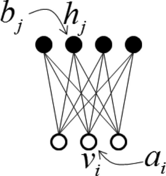
The RBM.
Given a training set of state vectors, the weights and biases in an RBM can be learned following the gradient of contrastive divergence. The learning rules are:
| (5) |
where the first expectation 〈.〉d is based on the data distribution and the second expectation 〈.〉r is based on the distribution of “reconstructed” data.
To incorporate temporal dependencies into the RBM, the CRBM [Taylor et al. (2006)] adds autoregressive connections from the visible and hidden variables of an individual to his/her historical variables. The CRBM simulates well human motion in the single agent scenario. However, it cannot capture the social influences on individual behaviors in the multiple agent scenario. Li et al. [Li et al. (2014)] proposed the ctRBM model for link prediction in dynamic networks. The ctRBM simulates the social influences by adding the prediction expectations of local neighbors on an individual into a dynamic bias. However, the visible layer of the ctRBMs does not take individual attributes as input. Thus, the ctRBM cannot directly predict human behaviors.
Meanwhile, social behavior has been studied recently, such as analysis of user interactions in Facebook [Viswanath et al. (2009)], activity recommendation [Lerman et al. (2012)], and user activity level prediction [Zhu et al. (2013)]. In Zhu et al. (2013), the authors focus on predicting users who have a tendency to lower their activity levels. This problem is known as churn prediction. Churn prediction aims to find users who will leave a network or a service. By finding such users, service providers could analyze the reasons for the intended attrition and could determine strategies to maintain such users in different applications, including online social games [Kawale et al. (2009)], QA forums [Yang et al. (2010)], etc. Our goal is not only to predict, but also to understand the roles of human behavior determinants, and to give explanations for predicted behaviors. In Barbieri et al. (2014), the authors provide the WTFW model, which generates explanations for user-to-user links, but not for human behaviors.
This paper is an extension of our conference paper published in ACM BCB 2015 [Phan et al. (2015b)]. The major extensions we have engaged are: (1) We have improved our previous ORBM model, not only so that it more accurately predicts human behavior, but also, so that it can generate explanations for each predicted behavior. We introduce a new temporal-smoothing social influence function to better capture the evolving of social influence over time. We further incorporate physical activity-based social influence into our function. We also introduce a new algorithm to quantitatively estimate the effects and roles of human behavior determinants in predicted behaviors. (2) An extensive experiment has been conducted on both real-world and synthetic health social networks to validate the effectiveness of our model, the roles of human behavior determinants, and the quality of generated explanations.
3. YesiWell Health Social Network and SMASH Ontology
3.1. YesiWell Health Social Network
Our health social network dataset was collected from Oct 2010 to Aug 2011, as a collaboration between PeaceHealth Laboratories, SK Telecom Americas, and University of Oregon, to record daily physical activities, social activities (i.e., text messages, competitions, etc.), biomarkers, and biometric measures (i.e., cholesterol, BMI, etc.) for a group of 254 individuals. Physical activities, including measurements of the number of walking and running steps, were reported every 15 minutes via a mobile device carried by each user. As mentioned in our Introduction, all users enrolled in an online social network, allowing them to befriend and communicate with each other. Users’ biomarkers and biometric measures were recorded via daily/weekly/monthly medical tests performed at home (i.e., individually) or at our laboratories. In total, we have approximately over 7 million data points of physical exercise, over 21,205 biomarker and biometric measurements, 1,371 friend connections, and 2,766 inbox messages. Our longitudinal study was conducted for 10 months. Albeit that such might seem a short interval, when compared with public social networks, i.e., Twitter and Facebook, our health social network is a unique, solid, and comprehensive multi-dimensional social network. The YesiWell network contains rich information from social activities, physical activities, and biomarkers and biometric measures, availing us unique access to verify statements about physical activity with recorded physical activity, and to compare statements about health with clinical measures of health.
In this paper, 33 features are taken into account (Table 1). All the features are summarized daily and weekly. The features are designed to capture the self-motivation of each user. Some of the key measures are as follows:
Personal ability: BMI, fitness, cholesterol, etc.
Attitudes: the number of off-line events in which each user participates, individual sending and receiving messages, the number of goals set and achieved, Wellness-score [Kil et al. (2012)], etc. Wellness-score is a measure to evaluate how well a user lives their life. Being active in social activities, setting and achieving more goals, and getting higher Wellness-score illustrate a healthier attitude of a user.
Intentions: the number of competitions each user joins, the number of goals set, etc. We measure intent to exercise in terms of competitions joined and goals set.
Effort: the number of exercise days, walking/running steps, the distances, and speed walked/run.
Withdrawal: an increase of BMI slope and/or a decrease of Wellness-score [Kil et al. (2012)] indicates a negative sign regarding the self-motivation. Users may give up.
Table 1.
Personal Attributes.
| Behaviors | #joining competitions | #exercising days | #goals set |
| #goals achieved | Σ(distances) | avg(speeds) | |
| #meet-up | #social games | ||
| Social Communications (the number of inbox messages) | Encouragement | Fitness | Followup |
| Competition | Games | Personal | |
| Study protocol | Progress report | Technique | |
| Social network | Meetups | Goal | |
| Wellness meter | Feedback | Heckling | |
| Explanation | Invitation | Notice | |
| Technical fitness | Physical | ||
| Biomarkers | Wellness Score | BMI | BMI slope |
| Wellness Score slope |
3.2. SMASH Ontology
Ontology [Gruber (1995); Studer et al. (1998)] is the formal specification of concepts and relationships for a particular domain (e.g., genetics). Prominent examples of biomedical ontologies include the Gene Ontology (GO [The gene ontology consortium (2001)]), Unified Medical Language System (UMLS [Lindberg et al. (1993)]), and more than 300 ontologies in the National Center for Biomedical Ontology (NCBO1). The encoded formal semantics in ontologies is primarily used for effective sharing and reusing of knowledge and data. They also can assist in the new research on systematic incorporation of domain knowledge in data mining, which is called semantic data mining [Dou et al. (2015)].
We have developed an ontology for health social networks, in the SMASH (Semantic Mining of Activity, Social, and Health data) project, based on the YesiWell study. Our general workflow of ontology development can be described as a top-down (knowledge-driven), followed by a bottom-up (data-driven) validation and refinement approach. In the SMASH ontology, we have focused on defining concepts that are associated with sustained weight loss, especially the ones related to continued intervention with frequent social contacts. We first follow the traditional top-down design paradigm by identifying the core concepts of three modules in the SMASH system: social networks, physical activity, and health informatics. We specify the core concepts and relationships related to overweight and obesity in these modules, such as biomedical measures, trends, online and off-line events, competitions, social community, support groups, etc. In the next step, these concepts and relationships are subsequently coded in the Web Ontology Language (OWL2) with Protégé3. In the last step, we further validate and refine our ontology design through the data we collected from our distributed personnel devices and web-based social network platform in YesiWell.
The three modules in our SMASH ontology, biomarker measures, physical activities, and social activities, can be described as follows:
Biomarkers: a collection of biomedical indicators that generally refer to biological states or conditions; in our case, specifically health conditions.
Social Activities: a set of interactions between social entities, either persons or social communities, who exchange thoughts and ideas, communicate information, and share emotions and experiences.
Physical Activities: any bodily activities involved in daily life. Some of the activities are conducted in order to enhance or maintain physical fitness and overall wellness/health.
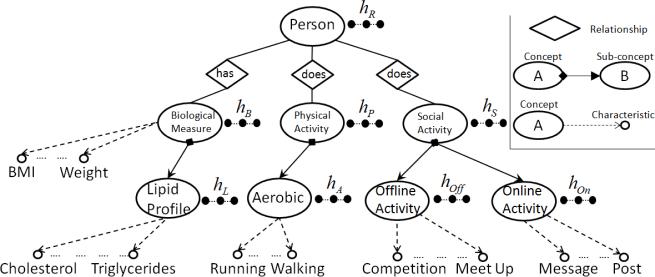
The SMASH ontology has been submitted to the NCBO BioPortal4. Figure 2 illustrates a partial view of the SMASH ontology and its hidden variables in the corresponding RBMs. (More details will be discussed in the next section.)
Figure 2.
Partial View of the SMASH Ontology and its Hidden Variables.
4. Ontology-based Representation Learning
In this section, we present our algorithm to learn user representations based on concepts and characteristics (properties) in ontologies. The representational primitives of ontologies are typically concepts, characteristics (datatype properties), and relationships (object properties). For instance, in Figure 2, the main concept is Person. With this concept, we have sub-concepts, relationships, and characteristics. Each person has a related concept Biological Measure which contains a set of characteristics such as BMI, weight, slope, wellness, etc. They are related to another concept, Social Activity, which contains sub-concepts, such as Offline Activity and Online Activity.
Given a health social network ontology H, the first step to utilize the formal semantics in deep learning is to learn the representation of all concepts, sub-concepts, and relationships given the characteristics. Our key hypothesis is that a concept or a sub-concept can be represented by its own characteristics, its sub-concepts, and its related concepts. In essence, is represented by a set of learnable hidden variables . The learning process of the is as follows. is composed of a set of characteristics , a set of sub-concepts , and a set of relationships . Let us denote as the union of all characteristics from its relationships , and as the union of all the hidden variables from its sub-concepts . The hidden variables can be learned from , , and by utilizing the RBMs as a deep learning model, since it very well fits our goals, which aim to generate a deeper analysis for human behavior prediction. By using the RBMs, the is considered as a hidden layer, and all the variables are considered as a visible layer in a RBM (Figure 1). The conditional probabilities of an and are given by:
| (6) |
| (7) |
where ai and bj are static biases, and Wij is a parameter associated with hj and vi. By denoting , the energy function of the RBM for is:
By using contrastive divergence [Hinton (2002)], we can train this RBM and learn all the parameters which are used to estimate the hidden variables . In fact, can be considered as the representation of . Note that we use normal distributions for the hidden variables in , because they will be used to learn the representation of the parent concepts of , denoted . may contain real-valued characteristics (datatype properties). So the consistency in the learning process is guaranteed. The representations of all the concepts and sub-concepts can be learned by applying the bottom-up greedy layer-wise algorithm [Hinton et al. (2006)] following the structure of the ontology H. For instance, in Figure 2, we can learn all the representations in the following order: hL, hA, hOff, hOn, first; then hB, hP, hS, and hR, finally.
Let us denote the root concept (e.g., Person) and its representation hR, which also is an individual representation. Different applications may have different settings. The challenge becomes how we organize the training data so that individual representation can be learned. In fact, the data of each user u will be collected in a set of time intervals T, denoted by where K is the set of all personal characteristics at all the concepts and sub-concepts. Du will be used to train the model. After training the model, for every t ∈ T we can navigate the following the ontology structure to estimate the representation of root concept hR which is also the representation of user u at time t. We train the model for each user independently. Each user will have different representations at different time intervals. In the next section, we show how to use those ontology-based user representations (i.e., RBMs) for human behavior prediction.
Our algorithm can learn the representations of individuals given different ontologies in different domain applications. In fact, our Ontology-based Representation Learning algorithm can learn the representation of any concept in a given ontology. Therefore, as long as we have an ontology, which represents or includes a “Person” concept, we can learn the representations of individuals. By offering this advanced ability, our model also can represent the hierarchical concept structures among biomedical and health domains.
5. ORBM+: Human Behavior Prediction with Explanations
In this section, we present how to conduct human behavior prediction with explanations based on user representations, which have been learned from the SMASH ontology. Given an online social network G = {U, E} where U is a set of all users and E is a set of edges. Every edge eu,m exists in E if u and m friend each other in G; otherwise eu,m does not exist. Each user has a set of individual representation features . In essence, is the hR which has been learned for each user in the previous Section. The social network G grows from scratch over a set of time points T = {t1, . . ., tm}. To illustrate this, we use ET = {Et1, . . . , Etm} to denote the topology of the network G over time, where Et is a set of edges which have been made until time t in the network, and ∀t ∈ T : Et ⊆ Et+1. For each user, the values of individual features in also change over time. We denote the values of individual features of a user u at time t as . At each time point t, each user u is associated with a binomial behavior . could be “decrease/increase exercise,” or “inactive/active in exercise.” will be clearly described in our experimental results section.
Problem Formulation
Given the health social network in M timestamps Tdata = {t – M + 1, . . ., t}, we would like to predict the behavior of all the users in the next timestamp t + 1. More formally, given we aim at predicting .
5.1. Self-motivation and Environmental Events
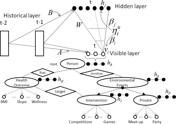
In order to model self-motivation of a user u, we first fully bipartite connect the hidden and visible layers via a weight matrix W (Figure 3). Then each visible variable vi and hidden variable hj will be connected to all the historical variables of u, denoted by where and k ∈ {1, . . ., N}. These connections are presented by the two weight matrices A and B (Figure 3). Each historical variable is the state of feature f of the user u at time point t – k. Note that all the historical variables are treated as additional observed inputs. The hidden layer can learn the correlations among the features and the effect of historical variables to capture self-motivation. This effect can be integrated into a dynamic bias:
| (8) |
which includes a static bias bj, and the contribution from the past of the social network. Bj is a |h| × |U| × N weight matrix which summarizes the autoregressive parameters to the hidden variable hj. This modifies the factorial distribution over hidden variables: bj in Eq. 3 is replaced with b̂j,t to obtain
| (9) |
where hj,t is the state of hidden variable j at time t, the weight Wij connects vi and hj. The self-motivation has a similar effect on the visible units. The reconstruction distribution in Eq. 4 becomes
| (10) |
where âi,t is also a dynamic bias:
| (11) |
Figure 3.
The ORBM+ model.
The effect of environmental events is composed of unobserved social relationships, unacquainted users, and the changing of social context [Christakis (2010); Phan et al. (2015a)]. In other words, a user can be influenced by any users via any features in health social networks. It is hard to precisely define the influences of environmental events. It is difficult to define straightforward statistical distribution functions, e.g., exponential function, Gaussian function, etc., to precisely present the influences of meet-up events, social games, competitions, etc., due to unobserved/hidden factors, such as undeclared friend connections and self-motivation. In fact, of all the actual friend relationships among participants, just a portion is observed in the YesiWell dataset, since users participated in many off-line events. Inspired by the SRBM model [Phan et al. (2015a)], we model the flexibility of implicit social influences, as well as self-motivation, as follows. The individual features of a user, denoted as , can be considered as the visible variables in the ORBM+ model (Figure 3). Given a user u, each visible variable vi and hidden variable hj are connected to all historical variables of all other users. It is similar to the self-motivation modeling: The influence effects of each user, and the social context on the user u, are captured via the weight matrices A and B. These effects can be integrated into the dynamic biases âi,t and b̂j,t in Eq. 11 and Eq. 8, as well. The dynamic biases in Eq. 8 and Eq. 11 become:
| (12) |
| (13) |
The quantitative environmental events, such as the number of competitions and meet-up events, are included as individual characteristics. Therefore, the effect of environmental events is better embedded into the model. Next, we will incorporate the social influence into our ORBM+ model.
5.2. Explicit Social Influences
It is well-known that individuals tend to be friends with people who perform behaviors similar to theirs (homophily principle). In addition, as shown in [Phan et al. (2014)], users differentially experience and absorb physical exercise-based influences from their friends. Therefore, the explicit social influences in health social networks can be defined as a function of the homophily effect and physical exercise-based social influences. Let us first define user similarity as follows.
Given two neighboring users u and m, a simple way to quantify their similarity is to applying a cosine function of their individual representations (i.e., vu and vm) and hidden features (i.e., hu and hv). The user similarity between u and m at time t, denoted st(u, m), is defined as:
| (14) |
where cost(·) is a cosine similarity function, i.e.,
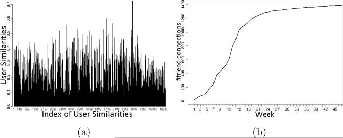
Figure 4a illustrates a sample of a user similarity spectrum of all the edges in our social network over time. We randomly select 35 similarities of neighboring users for each day in ten months. Apparently, the distributions are not uniform, and different time intervals present various distributions. To well qualify the similarity between individuals and their friends, it potentially requires a cumulative distribution function (CDF). In addition, our health social network is developed from scratch. As time goes by, each participant will have more connections to other users (Figure 4b). Thus a temporal smoothing is needed to better capture the explicit social influences. Eventually, we propose a statistical explicit social influence, denoted , of a user u at time t as follows:
where is a set of friends of user u, from the beginning until time t. ψt(m, u) is the physical exercise-based social influence of m on u at time t, which is derived by using the CPP model [Phan et al. (2014)]. st is the similarity between two arbitrary neighboring users in the social network at time t. p(st ≤ st(u, m)) represents the probability that the similarity is less than or equal to the instant similarity st(u, m). α and τ are two parameters to control the dynamics of η.
Figure 4.
A sample of cosine similarities (a) and cumulative number of friend connections (b) in our dataset.
5.3. Inference, Learning, and Prediction
Inference in the ORBM+ is no more difficult than in the RBM. The states of the hidden variables are determined both by the inputs they receive from the visible variables and from the historical variables. The conditional probability of hidden variables at time interval t can be computed, as in Eq. 8 and Eq. 9. The combination of the implicit and explicit social influences can be viewed as a linear adaptive bias: âi,t in Eq. 11 becomes
where βi is a parameter which presents the ability to observe the explicit social influences of user u given vi.
The energy function becomes:
Contrastive divergence is used to train the ORBM+ model. The updates for the symmetric weights, W, the static biases, a and b, the directed weights, A and B, are based on simple pairwise products. The gradients are summed over all the training time intervals t ∈ Ttrain = Tdata \ {t – M + 1, . . ., t – M + N}. The learning rules are summarized in Table 2.
Table 2.
Learning Rules
| Algorithm | Learning Rules |
|---|---|
| Contrastive Divergence | |
| Back-Propagation | |
On top of our model, we put an output layer for the user behavior prediction task. Our goal is to predict whether a user will increases or will decreases physical exercise levels. Thus the softmax layer contains a single output variable ŷ and binary target values: 1 for increases, and 0 for decreases. The output variable ŷ is fully linked to the hidden variables by weighted connections S, which includes |h| parameters sj. The logistic function is used as an activation function of ŷ as follows:
where c is a static bias. Given a user u ∈ U, a set of training vectors , and an output vector Y = {yt|t ∈ Ttrain}, the probability of a binary output yt ∈ {0, 1} given the input xt is as follows:
| (15) |
where ŷt = P(yt = 1|xt, θ).
A loss function to appropriately deal with the binomial problem is cross-entropy error. It is given by
| (16) |
In the final stage of training, Back-propagation is used to fine-tune all the parameters together. The derivatives of the objective C(θ) with respect to all the parameters over all the training cases t ∈ Ttrain are summarized in Table 2. In the prediction task, we need to predict the without observing the . In other words, the visible and hidden variables are not observed at the future time point t + 1. Thus we need a causal generation step to initiate these variables. Causal generation from a learned ORBM+ model can be done just like the learning procedure. In fact, we always keep the historical variables fixed and perform alternating Gibbs sampling to obtain a joint sample of the visible and hidden variables from the ORBM+ model. To start alternating Gibbs sampling, a good choice is to set vt = vt–1, (i.e., vt–1 is a strong prior of vt). This picks new hidden and visible variables that are compatible with each other and with the recent historical variables. Afterward, we aggregate the hidden variables to evaluate the output ŷ.
5.4. Explanation Generation
The success of human behavior intervention does not only depend on its accuracy in inferring and exploring users’ behaviors, but it also relies on how the deployed interventions are perceived by the users. Explanations increase the transparency of the intervention process and contribute to users’ satisfaction, and are facilitative in engaging users to the program.
The essence of explanations is to know the key characteristics or components that cause users to do some specific behaviors. In other words, an explanation can be defined as a list of characteristics which maximize the likelihood of a behavior being engaged by a user or a set of users. Recall that the log likelihood log P(Y|X, θ) that the users will do Y is maximized given all the characteristics X. Thus, X should be the best explanation for Y. However, X usually contains many characteristics in high dimensional data, that significantly reduces the interpret-ability of X. We need a solution to address the trade-off between the likelihood maximization and the complexity of X. Given a selection model f, the problem can be written as:
| (17) |
To address this issue, we utilize the Minimum Description Length (MDL) [Rissanen (1983)]. In the two-parts of MDL, we first use the explanation X′ to encode the observed data Y, and we then encode the explanation itself. We denote the encoding length of Y given X′ by L(Y, X′), and the encoding length of X′ by L(X′). As in Rissanen (1983), L(Y, X′) is the negative log-likelihood log P(Y|X′, θ) and L(X′) is given by |X′|log(|X|). MDL minimizes the combined encoding:
| (18) |
The complexity of explanation generating is NP-Hard. It is given by the following lemma.
Lemma 1
Finding the optimal explanation problem and the minimal value of the selection function is NP-Hard.
Proof 1
Given a set of elements {1, 2, . . ., m} (called the universe) and n sets whose union comprises the universe, the set cover problem [Motwani & Raghavan (1995)] is to identify the smallest number of sets whose union still contains all elements in the universe.
We can easily reduce the finding optimal explanation problem to the set cover problem by setting that x ∈ X is an item and X is the universe. x and X will be mapped into a likelihood space Y as: x :→ Yx = (P(y1|x, θ), . . ., P(yk|x, θ)), and X :→ YX = (P(y1|X, θ), . . ., P(yk|X, θ)) YX can be considered as a new universe, and Yx is an item in that universe. The problem now becomes finding the smallest number of items Yx whose union still covers the universe YX. That means we must have ∀i : P(yi|X′, θ) = P(yi|X, θ) where YX′ is the smallest union of items. In doing so, finding the optimal explanation is as hard as solving the corresponding instance of the set cover problem. This proves the NP-Hardness property of the given problem.
Since the finding optimal explanation problem is NP-Hard, we apply a heuristic greedy algorithm, which will add a new characteristic into the existing explanation so that the selection model MDL is minimized. Afterward, we are able to select the optimal explanation with a minimal MDL score.
6. Experimental Results
We have carried out a series of experiments in a real health social network to validate our proposed ORBM+ model (source codes and data5). We first elaborate about the experiment configurations, evaluation metrics, and baseline approaches. Then, we introduce the experimental results.
Experiment Configurations
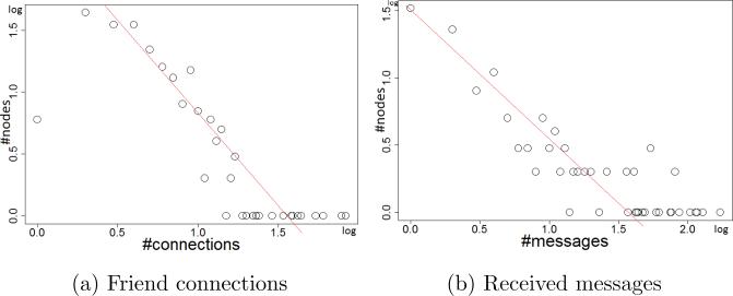
In our study, we take into account 33 personal attributes (Table 1). The personal social communications include 2,766 inbox messages, which are categorized into 20 different types. Figure 5 illustrates the distributions of friend connections, and #received messages in our data. They clearly follow the Power Law distribution. Note that, given a week, if a user exercises more than she did in the previous week, she is considered to be increasing exercise; otherwise, she will be considered to be decreasing exercise. The number of hidden units, and the number of previous time intervals N, respectively are set to 200 and 3. In the individual representation learning, the number of hidden units at all the concepts and sub-concepts in the ontology will double the number of visible units. The weights are randomly initialized from a zero-mean Gaussian with a standard deviation of 0.01. All the learning rates are set to 10−3. A contrastive divergence CD20 is used to maximize likelihood learning. We train the model for each user independently.
Figure 5.
Some distributions in our dataset.
Evaluation Metrics
In the experiment, we leverage the previous 10 weeks’ records to predict the behaviors of all the users (i.e., increase or decrease exercises) in the next week. The prediction quality metric, i.e., accuracy, is as follows:
where yi is the true user activity of the user ui, and ŷi denotes the predicted value, and I is the indication function.
Competitive Prediction Models
We compare the ORBM+ model with the conventional methods reported in Shen et al. (2012). The competitive methods are divided into two categories: personalized behavior prediction methods and socialized behavior prediction methods. Personalized methods only leverage individuals’ past behavior records for future behavior predictions. Socialized methods use both one person's past behavior records and his or her friends’ past behaviors for predictions. Specifically, the five models reported in Shen et al. (2012) are the Socialized Gaussian Process (SGP) model, the Socialized Logistical Autoregression (SLAR) model, the Personalized Gaussian Process (PGP) model, the Logistical Autoregression (LAR) model, and the Behavior Pattern Search (BPS) model.
We also consider the RBM related extensions, i.e., the CRBM [Taylor et al. (2006)] and ctRBM [Li et al. (2014)], as competitive models. The CRBM can be directly applied to our problem by ignoring the implicit and explicit influences in our SRBM+ model. Since the ctRBM cannot directly incorporate individual attributes with social influences to model human behaviors, we only can apply its social influence function into our model. In fact, we replace our statistical explicit social influence function with the ctRBM's social influence function. We call this version of ctRBM a Socialized ctRBM (SctRBM). We also compare the ORBM+ model with our previous works, SRBM in Phan et al. (2015a) and ORBM in Phan et al. (2015b).
6.1. Validation of the ORBM+ Model for Prediction
Our task of validation focuses on two key issues: (1) Which configurations of the parameters α and τ produce the best-fit social influence distribution? and (2) Is the ORBM+ model better than the competitive models, in terms of prediction accuracy? We carry out the validation through two approaches. One is to conduct human behavior prediction with various settings of α and τ. By this we look for an optimal configuration for the statistical explicit social influence function. The second validation is to compare our ORBM+ model with the competitive models in terms of prediction accuracy.
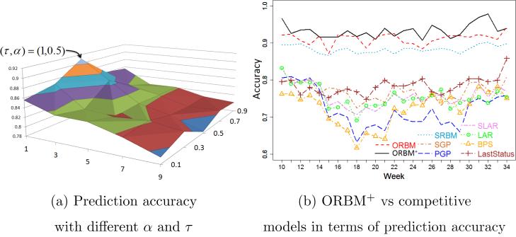
Figure 6a illustrates the surface of the prediction accuracy of the ORBM+ model, with variations of the two parameters α and τ on our health social network. We observed that the smaller values of τ tend to have higher prediction accuracies. This is quite reasonable, since the more recent behaviors have stronger influences. The temporal smoothing parameter τ has similar effects to a time decay function [Zhu et al. (2013)]. Meanwhile, the middle range values of α offer better prediction accuracies. Clearly, the optimal setting values of α and τ are 0.5 and 1 respectively.
Figure 6.
Validation of the ORBM+ model.
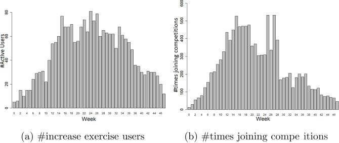
To examine the efficiency, we compare the proposed ORBM+ model with the competitive models, in terms of human behavior prediction. Figure 6c shows the accuracy comparison over 37 weeks in our health social network. It is clear that the ORBM+ outperforms the other models. The accuracies of the competitive models tend to drop in the middle period of the study. All the behavior determinants and their interactions potentially become stronger, since all the users improve their activities, such as walking and running, participating in more competitions, etc. (Figure 7) in the middle weeks. Absent or insufficient modeling of one of the determinants, or of one of their interactions, results in a low and unstable prediction performance. Therefore, competitive models do not well capture the social influences and environmental events. Meanwhile, the ORBM+ model comprehensively models all the determinants. So, the correlation between the personal attributes and the implicit social influences can be detected by the hidden variables. Thus, much information has been leveraged to predict individual behaviors. In addition, our prediction accuracy stably increases over time. That means our model well captures the growing of our health social network (Figure 4b). Consequently our model achieves higher prediction accuracy and a more stable performance. The ORBM+ model outperforms our previous ORBM model because of the new temporal-smoothing social influence function, which better captures the explicit social influences in our health social network. Overall, the ORBM+ model achieves the best prediction accuracy in average as 0.9332.
Figure 7.
The distributions of users’ activities.
6.2. The Effectiveness of User Representation Learning
In Figure 6b, the ORBM+ outperforms the SRBM, which does not learn user representation from the SMASH ontology, by 4.94% (0.8941 vs 0.9435). This is because ontology-based user representation provides better features, which encode semantics of the data structure from domain knowledge to the ORBM+ model. Even when we stack another hidden layer on the SRBM, the accuracy and the cross-entropy error are not (or are not much) improved, compared with the effect of ontology-based user representation. Consequently, we can conclude that: (1) The SMASH ontology helps us to organize data features in a suitable way; (2) Our algorithm can learn meaningful user representations from ontologies; and (3) Meaningful user representations can further improve accuracies of deep learning approaches for human behavior prediction.
6.3. Synthetic Health Social Network
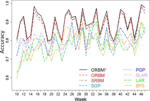
To illustrate that the ORBM+ model can be generally applied on different datasets, we perform further experiments on a synthetic health social network. To generate the synthetic data, we use the software Pajek6 to generate graphs under the Scale-Free/Power Law Model, which is a network model whose node degrees follow the Power Law distribution, or at least do asymptotically. However the vertices in the current synthetic graph do not have individual features similar to the real-word YesiWell data. An appropriate solution to this problem is to apply a graph-matching algorithm to map pairwise vertices between the synthetic and real social networks. In order to do so, we first generate a graph with 254 nodes, in which the average node degree is 5.4 (i.e., similar to the real YesiWell data). Then, we apply PATH [Zaslavskiy et al. (2008)], which is a very well-known and efficient graph-matching algorithm, to find a correspondence between vertices of the synthetic network and vertices of the YesiWell network. The source code of the PATH algorithm is available in the graph-matching package, GraphM7. Then, we can assign all the individual features and behaviors of real users to corresponding vertices in the synthetic network. Consequently, we have a synthetic health social network that imitates our real-world dataset. Figure 8 shows the accuracies of the conventional models, SRBM model, the ORBM model, and the ORBM+ model on the synthetic data. We can see that the ORBM+ model still outperforms the other models in terms of the prediction accuracy.
Figure 8.
Accuracies on the synthetic data.
6.4. Validation of Behavior Determinants and Explanations
6.4.1. Reliability of Behavior Determinants
One of our main goals is to validate the reliability of the human behavior determinants that are learned in our model. We illustrate this in a comparative experiment, which is to say: each determinant is independently used in the ORBM+ model to predict behaviors of the users. The ORBM+ model provides a natural way to address this. The effects of human behavior determinants are reflected via the ways we formulate the dynamic biases. To evaluate the effect of self-motivation on predicted behaviors, we compute the output variable ŷt+1 by using the dynamic biases b̂j,t and âi,t, which are in the forms of Eq. 8, 11. This means we only use the self-motivation effect to predict the behaviors of the users. Similarly, we can evaluate the effects of implicit social influences, explicit social influences, and environmental events. The corresponding dynamic biases for each human behavior determinant are summarized in Table 3. We use ŷt+1, self, ŷt+1, im, ŷt+1, ex, and ŷt+1, env to denote the output variable ŷt given corresponding determinants. With regard to the effect of environmental events, we use the number of joined competitions, meet-up events, and social games to evaluate the output variable ŷt+1, env.
Table 3.
Dynamic Biases of Human Behavior Determinants
| Determinants (output variable) | Dynamic biases |
|---|---|
| Self-motivation (ŷt+1,self) |
|
| Implicit social influence (ŷt+1,im) |
|
| Explicit social influence (ŷt+1,ex) |
|
| Environmental events (ŷt+1,env) | only use #competitions,#meet-up events, and #social games in the ORBM+ model |
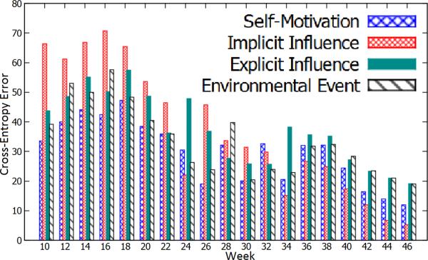
Figure 9 illustrates the cross-entropy errors in Eq. 16 of four determinants over 37 weeks of our data. We observed that self-motivation is more reliable than other determinants in terms of motivating users to increase their exercises in the first 10 weeks. This is because it achieves the best cross-entropy errors. Meanwhile, the implicit social influence is not effective in this period, since the users have not developed enough implicit relationships (i.e., highest cross-entropy errors). However, from the 24th week, the implicit social influence becomes one of the most reliable determinants, since it achieves the lowest cross-entropy errors. This phenomenon shows the important role of the implicit social influences in health social networks. In the meantime, the explicit social influences and environmental events behave as connecting factors, which not only influence the behaviors of users, but also associate the self-motivation and the implicit social influences together. In addition, the evolution of the determinants suggests a strong interaction among them, since there are no either absolutely reliable nor absolutely unreliable determinants.
Figure 9.
The cross-entropy errors of the human behavior determinants.
In obvious, we discover three meaningful observations: (1) The ORBM+ model enables the modeling of expressive correlations between determinants; (2) The self-motivation is especially important at the beginning; and (3) The implicit social influence will become one of the most reliable determinants, if the users have enough time to develop their relationships.
6.4.2. Human Behavior Explanations
We have shown that the ORBM+ model not only achieves a significantly higher prediction accuracy, compared with the conventional models, but it also offers a deep understanding of the human behavior determinants. That is a breakthrough in human behavior modeling in health social networks. In this section, we focus on giving explanations for human behaviors. The concerned questions are: “which are the key characteristics leading to the increasing or decreasing exercises of the users in the next week?” and “do these key characteristics offer a higher prediction accuracy with more interpretable results compared with the original personal characteristics?”
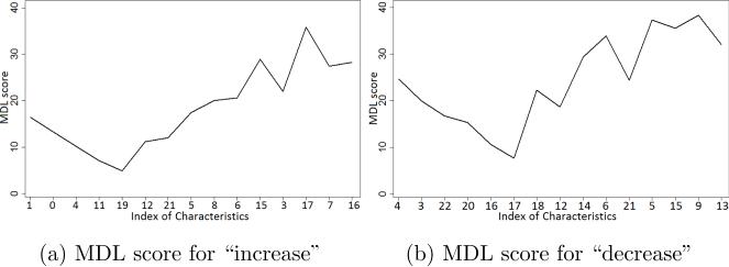
For instance, given the 9th week, the users will be classified into two groups which are predicted as increase exercise users and predicted as decrease exercise users in the next week. We then extract the key characteristics for each group by applying our algorithm based on MDL (Sec. 5.4). Figure 10a illustrates the scores of MDL the users who are predicted as increase exercises in the next week. We achieve the minimal value of the MDL given the list of characteristics8 {1, 0, 4, 11, 19} which is equivalent to {#exercise days, #competitions, Wellness-score, #competition messages, #progress reports}. Meanwhile, for the users for whom the model predicted a decrease in exercise, we obtain the minimal value of the MDL given the list of characteristics {4, 3, 22, 20, 16} which is equivalent to {Wellness-score, BMI slope, #invitations, #heckling messages, #goal messages} (Figure 10b).
Figure 10.
The scores of the MDL for predicted behaviors of the users at the 9th week.
To validate the interpret-ability of key characteristics extracted by our algorithms and models, we compare the decision trees extracted by interpretable classifiers from original personal characteristics and human behavior determinants in terms of classification and prediction accuracies. The interpretable classification models we used are: (1) Decision trees (DT) [Breiman et al. (1984)], which is a classical interpretable classifier; and (2) Ism_td [Van Assche & Blockeel (2007)], which is the state-of-the-art tree-based interpretable classification model. Table 4 illustrates the accuracies of the classification on predicted behaviors and the prediction, given actual behaviors of the users. The tree's depth is the maximal number of layers from the root of decision trees, which are generated by the DT and Ism_td algorithms. We can consider that, given the same prediction accuracy, the smaller the depth of the tree, the more interpretable the tree is. It is also true that, given the same depth, more accurate the tree in terms of classification and prediction, the more interpretable the tree is. In Table 4, we can see that by applying the DT and Ism_td algorithms on key characteristics, they achieve significantly better classification and prediction accuracies, given different values of tree's depth. In this point of view, the key characteristics extracted by our algorithm can be used to generate better interpretable decision-trees compared with the original personal characteristics. An example of generated decision trees from the Ism_td model is made available here9.
Table 4.
Classification and Prediction Accuracies of Interpretable Classifiers in the Whole Dataset
| Tree's Depth | 5 | 10 | 15 | 20 | |||||
|---|---|---|---|---|---|---|---|---|---|
| Classifier | DT | Ism_td | DT | Ism_td | DT | Ism_td | DT | Ism_td | |
| Personal Characteristics | Classification | 0.554 | 0.607 | 0.604 | 0.657 | 0.617 | 0.685 | 0.625 | 0.707 |
| Prediction | 0.494 | 0.558 | 0.569 | 0.57 | 0.587 | 0.605 | 0.593 | 0.631 | |
| Key Characteristics | Classification | 0.684 | 0.881 | 0.756 | 0.907 | 0.777 | 0.925 | 0.778 | 0.936 |
| Prediction | 0.635 | 0.801 | 0.728 | 0.838 | 0.748 | 0.886 | 0.751 | 0.860 | |
7. Conclusions
This paper introduces ORBM+, a novel ontology-based deep learning model for human behavior prediction and explanation in health social networks. By incorporating all human behavior determinants - self-motivation, implicit and explicit social influences, and environmental events - our model predicts the future activity levels of users more accurately and stably than conventional methods. We contribute novel techniques to deal with structural domain knowledge (i.e., ontologies) and human behavior modeling. Our experiments in real-world and synthetic health social networks discover several meaningful insights: (1) User representations based on ontologies can further improve accuracies of deep learning approaches for human behavior prediction; (2) The ORBM+ model expressively represents all the determinants and their correlations; and (3) Personal key characteristics which are extracted by our model are reliable, and they can be used to generate better explanations compared with original personal characteristics for human behaviors.
Acknowledgements
This work is supported by the NIH grant R01GM103309. The authors appreciate the anonymous reviewers for their extensive and informative comments to help improve the paper. The authors also appreciate the contributions of Xiao Xiao and Nafisa Chowdhury.
Footnotes
Publisher's Disclaimer: This is a PDF file of an unedited manuscript that has been accepted for publication. As a service to our customers we are providing this early version of the manuscript. The manuscript will undergo copyediting, typesetting, and review of the resulting proof before it is published in its final citable form. Please note that during the production process errors may be discovered which could affect the content, and all legal disclaimers that apply to the journal pertain.
References
- Bandura A. Human agency in social cognitive theory. The American Psychologist. 1989;44:1175–84. doi: 10.1037/0003-066x.44.9.1175. [DOI] [PubMed] [Google Scholar]
- Barbieri N, Bonchi F, Manco F. Who to follow and why: Link prediction with explanations. KDD '14. 2014:1266–1275. [Google Scholar]
- Breiman L, Friedman JH, Olshen RA, Stone CJ. Classification and Regression Trees. Wadsworth International Group; 1984. [Google Scholar]
- Christakis N. The hidden influence of social networks. TED2010. 2010 URL: http://www.ted.com/talks/nicholas_christakis_the_hidden_influence_of_social_networks.
- Christakis N, Fowler J. The spread of obesity in a large social network over 32 years. The New England Journal of Medicine. 2007;357:370–9. doi: 10.1056/NEJMsa066082. [DOI] [PubMed] [Google Scholar]
- Dou D, Wang H, Liu H. Semantic Data Mining: A Survey of Ontology-based Approaches. ICSC'15. 2015:244–251. [Google Scholar]
- Fichman R, Kemerer C. The illusory diffusion of innovation: An examination of assimilation gaps. Information Systems Research. 1999;10:255–275. [Google Scholar]
- Gruber T. A translation approach to portable ontology specifications. Knowledge Acquisition. 1993;5:199–220. [Google Scholar]
- Gruber TR. Toward principles for the design of ontologies used for knowledge sharing? International Journal of Human-computer Studies. 1995;43:907–928. [Google Scholar]
- Hinton G. Training products of experts by minimizing contrastive divergence. Neural Computation. 2002;14:1771–1800. doi: 10.1162/089976602760128018. [DOI] [PubMed] [Google Scholar]
- Hinton G, Osindero S, Teh Y-W. A fast learning algorithm for deep belief nets. Neural Computation. 2006;18:1527–1554. doi: 10.1162/neco.2006.18.7.1527. [DOI] [PubMed] [Google Scholar]
- Huang J, Cheng X-Q, Shen H-W, Zhou T, Jin X. Exploring social influence via posterior effect of word-of-mouth recommendations. WSDM'12. 2012:573–582. [Google Scholar]
- Kawale J, Pal A, Srivastava J. Churn prediction in mmorpgs: A social influence based approach. CSE'09. 2009:423–428. [Google Scholar]
- Kil D, Shin F, Piniewski B, Hahn J, Chan K. Impacts of social health data on predicting weight loss and engagement.. O'Reilly StrataRx Conference; San Francisco, CA. 2012. [Google Scholar]
- Lecun Y, Bottou L, Bengio Y, Haffner P. Gradient-based learning applied to document recognition. Proceedings of the IEEE. 1998;86:2278–2324. [Google Scholar]
- Lerman K, Intagorn S, Kang J-K, Ghosh R. Using proximity to predict activity in social networks. WWW'12 Companion. 2012:555–556. [Google Scholar]
- Li X, Du N, Li H, Li K, Gao J, Zhang A. A deep learning approach to link prediction in dynamic networks. SDM'14. 2014:289–297. [Google Scholar]
- Lindberg D, Humphries B, McCray A. The Unified Medical Language System. Methods of Information in Medicine. 1993;32:281–291. doi: 10.1055/s-0038-1634945. [DOI] [PMC free article] [PubMed] [Google Scholar]
- Marshall A, Eakin E, Leslie E, Owen N. Exploring the feasibility and acceptability of using internet technology to promote physical activity within a defined community. Health Promotion Journal of Australia. 2005;2005:82–4. doi: 10.1071/he05082. [DOI] [PubMed] [Google Scholar]
- Motwani R, Raghavan P. Randomized algorithms. Cambridge University Press; New York, USA: 1995. [Google Scholar]
- Pate R, Pratt M, Blair S, et al. Physical activity and public health. a recommendation from the centers for disease control and prevention and the american college of sports medicine. The Journal of the American Medical Association. 1995;273:402–7. doi: 10.1001/jama.273.5.402. [DOI] [PubMed] [Google Scholar]
- Phan N, Dou D, Piniewski B, Kil D. Social restricted boltzmann machine: Human behavior prediction in health social networks. ASONAM'15. 2015a:424–431. doi: 10.1007/s13278-016-0379-0. [DOI] [PMC free article] [PubMed] [Google Scholar]
- Phan N, Dou D, Wang H, Kil D, Piniewski B. Ontology-based deep learning for human behavior prediction in health social networks. ACM BCB'15. 2015b:433–442. doi: 10.1016/j.ins.2016.08.038. [DOI] [PMC free article] [PubMed] [Google Scholar]
- Phan N, Dou D, Xiao X, Piniewski B, Kil D. Analysis of physical activity propagation in a health social network. CIKM'14. 2014:1329–1338. [Google Scholar]
- Poon H, Domingos P. Sum-product networks: A new deep architecture. IEEE ICCV Workshops. 2011:689–690. [Google Scholar]
- Rissanen J. A universal prior for integers and estimation by minimum description length. The annals of statistics. 1983;14:416–431. [Google Scholar]
- Shen Y, Jin R, Dou D, Chowdhury N, Sun J, Piniewski B, Kil D. Socialized gaussian process model for human behavior prediction in a health social network. ICDM'12. 2012:1110–1115. doi: 10.1007/s10115-015-0910-z. [DOI] [PMC free article] [PubMed] [Google Scholar]
- Smolensky P. Information processing in dynamical systems: Foundations of harmony theory. Parallel Distributed Processing: Explorations in the Microstructure of Cognition. 1986;1:194–281. [Google Scholar]
- Studer R, Benjamins VR, Fensel D. Knowledge engineering: principles and methods. Data & knowledge engineering. 1998;25:161–197. [Google Scholar]
- Taylor G, Hinton G, Roweis S. Modeling human motion using binary latent variables. NIPS'06. 2006:1345–1352. [Google Scholar]
- The gene ontology consortium Creating the gene ontology resource: design and implementation. Genome Research. 2001;11:1425–1433. doi: 10.1101/gr.180801. URL: http://dx.doi.org/10.1101/gr.180801. doi:10.1101/gr.180801. [DOI] [PMC free article] [PubMed] [Google Scholar]
- Van Assche A, Blockeel H. Seeing the forest through the trees: Learning a comprehensible model from an ensemble. ECML'07. 2007;4701:418–429. [Google Scholar]
- Viswanath B, Mislove A, Cha M, Gummadi K. On the evolution of user interaction in facebook. WOSN'09. 2009:37–42. [Google Scholar]
- Welling M, Rosen-Zvi M, Hinton G. Exponential family harmoniums with an application to information retrieval. NIPS'04. 2004:1481–1488. [Google Scholar]
- Yang J, Wei X, Ackerman M, Adamic L. Activity lifespan: An analysis of user survival patterns in online knowledge sharing communities. ICWSM'10. 2010 [Google Scholar]
- Zaslavskiy M, Bach F, Vert J-P. A path following algorithm for graph matching. IEEE Transactions on Pattern Analysis and Machine Intelligence. 2008;5099:329–337. doi: 10.1109/TPAMI.2008.245. [DOI] [PubMed] [Google Scholar]
- Zhu Y, Zhong E, Pan S, Wang X, Zhou M, Yang Q. Predicting user activity level in social networks. CIKM'13. 2013:159–168. [Google Scholar]


