Picosecond Photobiology: Watching a Signaling Protein Function in Real Time via Time-Resolved Small- and Wide-Angle X-ray Scattering

Abstract

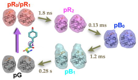
The capacity to respond to environmental changes is crucial to an organism’s survival. Halorhodospira halophila is a photosynthetic bacterium that swims away from blue light, presumably in an effort to evade photons energetic enough to be genetically harmful. The protein responsible for this response is believed to be photoactive yellow protein (PYP), whose chromophore photoisomerizes from trans to cis in the presence of blue light. We investigated the complete PYP photocycle by acquiring time-resolved small and wide-angle X-ray scattering patterns (SAXS/WAXS) over 10 decades of time spanning from 100 ps to 1 s. Using a sequential model, global analysis of the time-dependent scattering differences recovered four intermediates (pR₀/pR₁, pR₂, pB₀, pB₁), the first three of which can be assigned to prior time-resolved crystal structures. The 1.8 ms pB₀ to pB₁ transition produces the PYP signaling state, whose radius of gyration (R_g = 16.6 Å) is significantly larger than that for the ground state (R_g = 14.7 Å) and is therefore inaccessible to time-resolved protein crystallography. The shape of the signaling state, reconstructed using GASBOR, is highly anisotropic and entails significant elongation of the long axis of the protein. This structural change is consistent with unfolding of the 25 residue N-terminal domain, which exposes the β-scaffold of this sensory protein to a potential binding partner. This mechanistically detailed description of the complete PYP photocycle, made possible by time-resolved crystal and solution studies, provides a framework for understanding signal transduction in proteins and for assessing and validating theoretical/computational approaches in protein biophysics.

Graphical Abstract

INTRODUCTION

In May 2014, the number of structures deposited in the Protein Data Bank passed 100,000.^1,2 While static structures provide some clues regarding how proteins execute their designed function, much is left to the imagination. Indeed, proteins are not static macromolecules, but undergo conformational changes whose choreographed motions can, for example, gate the transport of substrate to and from the active site and can modulate over time the activity of that site. One of the grand challenges for the 21st century is to develop a mechanistic understanding into how proteins function at the molecular level. To that end, it is crucial to characterize how a protein’s structure evolves over time, i.e., we wish to watch a protein as it functions.

Time-resolved Laue crystallography studies using X-ray pulses available at third-generation synchrotrons have demonstrated the ability to recover protein structures of short-lived intermediates with 150 ps time resolution and near-atomic spatial resolution.^3–7 Recent studies at the Linear Coherent Light Source (LCLS), an X-ray free-electron laser, have extended the time-resolution achievable with crystallography down to a few hundred femtoseconds.^8,9 However, the highly ordered crystal packing arrangement that makes this high-resolution structure determination possible also constrains motion of the protein. Therefore, proteins whose function requires large-amplitude motion, including many allosteric or signaling proteins, are not free to execute their designed function when constrained within a protein crystal. To complement time-resolved Laue crystallography studies of proteins, we have developed the infrastructure required to probe protein structure changes in solution via picosecond time-resolved small- and wide-angle x-ray scattering (SAXS/ WAXS).¹⁰ Time-resolved scattering studies of proteins have also been pursued at the LCLS,^11,12 where the time resolution achievable in the WAXS region has been extended down to a few hundred femtoseconds. Since the structural information contained in X-ray scattering patterns is inherently one-dimensional, it is not possible to reconstruct high-resolution three-dimensional protein structures from these data. Nevertheless, both SAXS and WAXS can track the dynamics of structural transitions in solution; however, SAXS is needed to characterize changes in the size and shape of the protein that arise from those structural transitions. Here, we use time-resolved SAXS/WAXS to characterize, over 10 decades of time, the complete photocycle of photoactive yellow protein (PYP) in solution, including its crystal-inaccessible, long-lived signaling state.

PYP, a small (14-kD) blue-light receptor first found in the purple sulfur bacterium Halorhodospira halophila,¹³ has long served as a model system for investigating signaling in proteins¹⁴ and has been studied with time-resolved spectroscopic,^15–17 crystallographic,^18–20 and scattering²¹ methods. This bacterium swims away from blue light and toward photosynthetically useful green and near-infrared light.²² The absorbance spectrum of PYP matches the action spectrum for negative phototaxis,²² suggesting that PYP is responsible for the signal that causes this halophile to swim away from photons energetic enough to be genetically harmful. Upon absorbing a blue photon, the p-coumaric acid (pCA) chromophore in PYP undergoes trans to cis photoisomerization, an ultrafast event that triggers a reversible photocycle involving both red- and blue-shifted PYP intermediates. A recent time-resolved Laue crystallography study of PYP characterized its complete photocycle from 100 ps to 1 s at an unprecedented level of structural detail.⁵ Crystal structures of the PYP ground state (pG) and the last intermediate accessible in the crystal (pB₀) are shown in Figure 1 A,B, respectively. Strain induced by photoisomerization of pCA breaks two strong hydrogen bonds involving Glu46 and Tyr42 and the pCA chromophore, allowing its phenolate to swing toward and form a hydrogen bond with Arg52, which in turn pivots to the side and exposes the phenolate to the solvent. This solvent exposure leads to protonation and a blue-shift of the pCA chromophore and also allows a single water molecule to penetrate into the protein interior and hydrogen bond with Glu46 and Tyr42. The presence of this internal water blocks return to the ground state and prolongs the lifetime of this intermediate. The energy stored in this intermediate is sufficient to drive the protein back to the ground state, thereby completing its photocycle and making this process fully reversible.

Figure 1.

Crystal structures of PYP. (A) Structure of PYP in its pG ground state (PDB ID: 2ZOH). (B) Structure of PYP in its pB₀ state (PDB ID: 4BBV), as determined by time-resolved Laue crystallography.⁵ In this state, a water molecule penetrates into the interior of the protein and hydrogen-bonds to Glu46 and Tyr42. A second water molecule hydrogen bonds to the pCA phenolate oxygen, which is protonated in this state. The surfaces of both figures are rendered as glass and the backbone as ribbon. The pCA chromophore and Arg52, along with their hydrogen-bonding partners, are rendered as licorice. Dashed blue lines depict hydrogen bonds. The 25-residue N-terminal domain, colored orange, caps the β-scaffold of this sensory protein.²³

Because crystal packing forces constrain global motion of the protein, the longest-lived intermediate accessible in the crystal is denoted pB₀; the zero subscript reflects our view that this intermediate is not the true signaling state, but the precursor to it. When photoisomerization is triggered in solution, where PYP is free of crystal packing constraints, the transition to the true signaling state is accessible. The time-resolved SAXS/ WAXS patterns of PYP in solution reported here unveil the global structure of each intermediate in the PYP photocycle. The structural change associated with the pB₀ to pB₁ transition is dramatic, the scale of which imposes strict constraints on structural models for the signaling state of PYP.

EXPERIMENTAL SECTION

Picosecond time-resolved SAXS/WAXS “snapshots” of PYP were acquired on the BioCARS beamline at the Advanced Photon Source (APS) using the pump–probe method, as described previously.^10,24 Briefly, a ~100 ps duration, 390 nm, ~3 mJ·mm⁻² laser pulse photo activated a ~50 mg·ml⁻¹ PYP solution in a capillary (pump), after which a suitably delayed, ~117 ps duration, 12 keV X-ray pulse (probe) passed through the pump-illuminated volume. The time-resolved X-ray scattering pattern produced at each time delay was recorded on a mar165 CCD. The time resolution achievable is determined by the convolution of the pump and probe pulses, which is ~150 ps fwhm. Time-resolved X-ray scattering images were recorded over 10 decades of time spanning from 100 ps to 1 s with laser “off” images interleaved among laser “on” images. After applying polarization, geometry, and detector nonuniformity corrections to the 2D scattering images, the measured scattering intensities, I [photons/ pixel], were binned and averaged as a function of the scattering vector magnitude, q = (4π sin θ)/ λ, where 2θ is the scattering angle and λ is the wavelength of the incident X-ray beam. The data reported here were merged from three separate runs with each focusing on different but overlapping time ranges. Time delays of 10 μs and beyond were acquired when the APS operated in its 24-bunch standard operating mode. To speed data acquisition in that mode, the high-speed chopper height was lowered to transmit a burst of 11 X-ray pulses spanning 1.5 μs, a duration that is short compared to the targeted time delays. The sample capillary was translated 240 μm along its length to a fresh spot between each pump–probe pair. After exposure to 100 pump–probe pairs along a 24 mm stretch of the capillary (1100 X-ray pulses), the mar165 CCD X-ray detector was read, a syringe pump pushed fresh protein into the capillary, and the fast linear translation stage (Parker MX80) returned to the beginning of its stroke to start acquiring the next image in the series. Due in part to the relatively slow readout time of the detector, the time between images was about 4 s, which was long compared to the ground-state recovery time for PYP. Thanks to the 12 ms dwell time at each spot, time delays out to 10 ms could be acquired at a pulse repetition frequency of 41 Hz. To acquire time delays beyond 10 ms, the pulse repetition frequency was reduced to approximately the inverse of the pump–probe delay time. Time delays up to 10 μs were acquired when the APS operated in hybrid mode, which delivered an X-ray pulse approximately 4 times greater in flux than is available from the 24-bunch standard operating mode. To generate comparable image intensities when acquiring data in this mode, three strokes of the translation stage were integrated before reading the detector (comparable to ~1200 X-ray pulses in 24-bunch mode). Pump-induced scattering differences were generated by subtracting appropriately scaled scattering curves recorded without laser excitation from those recorded with laser excitation. The differences recorded at each time delay were averaged over 20 repeated measurements. Singular value decomposition (SVD) was employed to filter the data and improve the signal-to-noise ratio (S/N) of the scattering curves.

SAXS/WAXS images of the longest-lived PYP intermediate were recorded as a function of laser flux using a 473 nm CW laser (Optotronics I-VA-100-473). A motorized gradient neutral density filter controlled the power density of the focused laser beam. SAXS/WAXS images were acquired at each of five different levels of attenuation, each decreasing by approximately a factor of 2, with the power series repeated 50 times. A laser shutter (Uniblitz) opened 20 ms prior to each 11-bunch X-ray burst, with the SAXS/WAXS images read after 100 pump–probe pairs. The maximum power density delivered, 320 mW·mm⁻², was sufficient to saturate the population of the longest-lived intermediate.

A suite of applications developed by D. I. Svergun and coworkers^25–27 was used to reconstruct particle shapes consistent with the experimentally determined scattering curves for pG and each intermediate in the PYP photocycle. Briefly, scattering curves were input into GNOM²⁵ to produce files suitable for input into GASBOR.²⁶ This program was executed in reciprocal space mode (GASBORI) and produced ab initio low-resolution reconstructions of the protein structure. Ten independent annealing runs were executed for each state in the photocycle. Using DAMAVER,²⁷ the ensemble of models generated for each state were aligned and averaged to produce a 3-D model for each intermediate.

RESULTS

Time-resolved X-ray scattering differences recorded over 10 decades of time spanning from 100 ps to 1 s are shown in Figure 2A. The scattering differences have been scaled by q, which produces a quantity that is proportional to the differential number of photons detected in each q bin. According to global analysis of the scattering differences, the simplest model that can account for the time-resolved changes is a sequential four-state model (Figure 2B) that includes a time-dependent thermal signal. The rate coefficients in this four-state model were optimized by Marquardt–Levenberg nonlinear least-squares, and the species-specific scattering differences (Figure 2C) were recovered by linear least-squares. A thermal component is required because photoexcitation of the protein deposits sufficient energy to warm the surrounding solution by nearly 0.5 °C. The relatively large scattering differences produced by this T-jump disappear on the few millisecond to second time scale as excess heat diffuses out of the laser/X-ray interaction region. The thermal signal used in the global analysis (gray curve in Figure 2C) was measured experimentally and corresponds to a 1 °C increase in buffer temperature. The population dynamics for the intermediates (Figure 2D; smooth curves) account for the instrument response function (~150 ps fwhm) and pump saturation effects. Linear least-squares fitting of the five basis scattering patterns to the experimentally measured difference curves recovered time-dependent amplitudes (symbols) for each basis pattern. The symbols reproduce, within experimental error, the smooth curves over all 10 decades, confirming that this minimalist four-state sequential model is sufficient to describe the PYP photocycle in solution. Note that the S/N of the basis curves correlates with the number of frames in which they are represented.

Figure 2.

Time-resolved X-ray scattering of PYP in solution (50 mg·mL⁻¹; 150 mM NaCl; 20 mM sodium phosphate buffer, pH 6.0). (A) Scattering differences recorded over 10 decades of time. For clarity, not all time delays are shown. (B) Kinetic model used in the global analysis. The PYP photocycle is triggered by trans-to-cis photo-isomerization of the pCA chromophore (shown in center). The colors in panel A are blended according to the color code of intermediates in this kinetic model. (C) Scattering differences of intermediates recovered by global analysis of the data in panel A. The gray line corresponds to the thermal contribution to the scattering signal (ΔT = 1.0 °C). (D) Upper panel: the black triangles track the time-dependent relative change in the SAXS intensity at q = 0.11 Å⁻¹ (see black vertical line in panel A). The time scale is linear from –100 to 100 ps and logarithmic thereafter. Lower panel: time-dependent population of the intermediates (colored lines) and time-dependent temperature of the solution (gray line). The dashed line near zero time corresponds to the convolution of the laser and X-ray pulse, whose width determines the time resolution of the measurement.

The most prominent feature in these difference curves is found in the SAXS region, which is sensitive to protein size and shape. This feature is positive going at early time delays but becomes strongly negative at long time delays. The time-dependent amplitude of this feature is shown in the upper panel of Figure 2D, which was scaled relative to the absolute scattering curve for the ground state, pG. The rise time of this signal follows the integral of the instrument response function, suggesting that the associated protein structure change is prompt and faster than the ~150 ps time resolution achieved in this study. At long times, the scattering intensity of this feature decreases by about 10%, indicating a dramatic change in the global structure of the protein.

To characterize the structures of intermediates found in the PYP photocycle, it is crucial to determine the photoisomerization yield achieved in this study. The signaling-state yield was determined from pump-power-dependent scattering differences recorded after exposing PYP to a 20 ms duration, 473 nm laser pulse whose flux was varied nearly 20-fold up to saturation (Figure 3A). These curves are reproduced with high fidelity by a linear combination of two basis scattering vectors (Figure 3B): one representing the signaling-state scattering difference (green), and the other representing the thermal signal arising from the laser-induced change in the water temperature (gray). As expected, the thermal signal increases linearly with laser flux, while the protein signal saturates at high laser flux (Figure 3C). The amplitude of the difference signal at saturation provides the calibration needed to estimate the signaling-state yield in our picosecond time-resolved SAXS/WAXS study. Indeed, the pB₁ scattering curve in Figure 2B (cyan) is superimposable with the pB₁ curve in Figure 3B after dividing by 0.42; this value therefore represents the signaling-state yield achieved with picosecond pulse excitation.

Figure 3.

Pump-power-dependent X-ray scattering from the pB₁ signaling state. (A) Scattering differences acquired after photo-activation with five different power densities. (B) Protein (green) and thermal (gray) contributions to the scattering differences were obtained by global analysis of the differences in panel A. The population of the signaling state at the highest flux was assumed to be 100%. The thermal difference signal corresponds to ΔT = +1 °C. Overlapping the green curve is the scaled difference curve reported for pB₁ in Figure 2C (cyan). (C) Pump-power-dependent amplitudes of the protein (green) and thermal (gray) contributions to the scattering patterns in panel A. The scale factor (cyan triangle) required to put the time-resolved scattering differences reported for (pB₁ – pG) in Figure 2C on the same scale as the curve in Panel B corresponds to the signaling-state population achieved with the ~100 ps laser pulse used in the time-resolved study.

At the 50 mg·mL⁻¹ protein concentration used to obtain the relatively high S/N scattering curves reported here, the protein occupies about 3.7% of the solution volume. At this volume fraction, the so-called packing structure factor, S(q),^28,29 whose curvature depends on both volume fraction and interparticle interactions, distorts significantly the scattering pattern in the SAXS region. Before we can determine the size and shape of intermediates in the PYP photocycle, we must first correct for this distortion. To that end, we recorded the ground state scattering pattern of PYP at three protein concentrations differing by factors of 3 (Figure 4A). The three curves, after scaling according to concentration, are virtually superimposable in the WAXS region, but deviate significantly from each other in the SAXS region. In the absence of a packing structure factor effect, a Guinier plot of the scattering amplitude (natural log of intensity vs q²) in the low q region (q × R_g < 1.3) is expected to produce a linear curve whose slope is –R_g²/3, where R_g is the protein radius of gyration. A Guinier plot of the experimental scattering curves (Figure 4B), rescaled according to their relative concentration, reveals significant curvature in the Guinier region at high concentration; however, a quadratic extrapolation of the three curves to infinite dilution produces a linear curve, whose least-squares slope corresponds to an R_g of 14.69 ± 0.02 Å.

Figure 4.

Concentration dependence of PYP scattering. (A) Log–log plot of scattering intensities. The two lower concentrations were rescaled to the high-concentration curve according to the ratio of their concentrations. S(q) corresponds to the ratio of the scattering curve acquired at 50 mg·mL⁻¹ and its infinite dilution extrapolation. The gray shaded region corresponds to the Guinier region, i.e., where q ×R_g < 1.3. (B) Guinier plot of the scattering curves in panel A. The black line is a linear least-squares fit of the extrapolation to infinite dilution. The slope of this line corresponds to –R_g²/3.

The ratio of the scattering curve acquired at 50 mg·mL⁻¹ and its extrapolation to infinite dilution produces an experimental determination of the packing structure factor, S(q) (Figure 4A). This curve reveals increasing suppression of the scattering intensity with decreasing q and, if unaccounted for, reduces the slope of the Guinier plot. The magnitude of this suppression is greater than the ~25% suppression predicted at q = 0 by a hard-sphere model,³⁰ which implies repulsive protein–protein interactions. If we assume the structure factor is the same for all intermediates in the PYP photocycle, extrapolation to infinite dilution is readily accomplished by dividing I(q) for each intermediate by S(q).

Given our experimental determinations of both signaling-state yield and S(q), we constructed scattering curves for each intermediate in the PYP photocycle (Figure 5A), which are put on the same scale as pG and represent an extrapolation to the infinite dilution limit. Using GNOM, these curves up to q = 0.8 A⁻¹ were Fourier transformed to compute the distance distribution function p(r) shown in Figure 5B. Guinier plots of the curves in Figure 5A are shown in Figure 5C, with the corresponding slope and intercept translated to R_g and I₀ in Figure 5D. Owing to the large number of repeated measurements, the standard errors calculated for these quantities are quite small. Indeed, the ±1σ error bars in Figure 5D span a range less than or equal to the symbol size. For example, R_g for the pB₁ state is 16.58 ± 0.03 Å (the statistical uncertainty for this state is about 50% larger than that for pG). Elsewhere in the text, this value was rounded to 16.6 Å. The most dramatic changes in the protein structure clearly arise upon formation of pB₁.

Figure 5.

Scattering of PYP and intermediates in its photocycle. (A) Log–log plot of scattering intensities; corrected for the packing structure factor (50 mg·mL⁻¹). (B) Distance distribution function, p(r), computed from the curves in panel A using GNOM.²⁵ (C) Guinier plots of the scattering curves in panel A. (D) I₀ and R_g determined from linear least-squares fits of the Guinier plots in panel C. R_g (Å): pG (14.7); pR₀/pR₁ (14.5); pR₂ (14.7); pB₀, (15.0) and pB₁ (16.6). I₀ (relative to pG): pG (1.000); pR₀/pR₁ (0.998); pR₂ (1.000); pB₀ (0.996); and pB₁ (1.104). The error bars correspond to ±1σ.

The limited range of q represented in Guinier plots unveils fundamentally important quantities about protein size but not its shape. To gain insight into protein shape, we must look beyond the Guinier region. To that end, scattering data acquired at high protein concentration over a large dynamic range of q, which spans beyond the peak of the water ring, facilitated accurate buffer subtraction and accurate reconstruction of the protein shape.

Although the scattering curves for PYP and its photocycle intermediates are 1-D, they arise from 3-D objects. By comparing scattering patterns calculated theoretically for 3-D objects with a 1-D experimental scattering curve, it is possible to assess a range of sizes and shapes that are consistent with the 1-D scattering curve. To that end, the scattering curves in Figure 5A were processed using a suite of applications developed by D. I. Svergun and co-workers^25–27 to generate 3D reconstructions of the protein size and shape (see Experimental Section). Docked into both front and side views of these reconstructions (Figure 6) is the pG crystal structure with the 25-residue N-terminal domain colored orange (rendered with VMD).³¹ Clearly, the largest change in protein shape occurs during the pB₀ to pB₁ transition.

Figure 6.

GASBOR reconstruction of particle shape from the curves shown in Figure 5A. The front and side views are superimposed on the pG structure of PYP. The major and minor dimensions of the 3-D GASBOR models were estimated by linear-least-squares fitting an ellipsoid (a,b,c) to each model. Relative to pG, the magnitudes of the major axes are pR₀/pR₁ (0.996); pR₂ (1.011); pB₀, (1.047); and pB₁ (1.422).

DISCUSSION

The structural changes observed in this study are triggered by trans-to-cis photoisomerization of the pCA chromophore in PYP, which acts like a winch and promptly contracts the dimension of the protein along the long axis of the chromophore.^5,24 This primary event generates strain in the protein and launches a photocycle that ultimately leads to the signaling state of PYP. The simple four-state sequential model depicted in Figure 2B reproduces time-resolved scattering curves recorded over 10 decades of time with high fidelity, and the scattering patterns of the four intermediates detected, after proper scaling and correction for packing structure factor effects (Figure 5A), depict the global structural changes occurring during the PYP photocycle.

It is well-known that the on-axis scattering amplitude for a single particle, irrespective of its size and shape, is proportional to the square of the number of excess electrons contained within that particle (i.e., excess relative to the number of electrons contained in the volume displaced by that particle),³² which is related to electron density and volume according to

$$I_0={(\mathrm{\Delta }{n}_{\mathrm{e}})}^2={(\mathrm{\Delta }\rho )}^2{V}^2$$ (1)

where I₀ is the forward scattering at q = 0, Δn_e is the number of excess electrons, Δρ corresponds to the electron density difference between the particle and its surroundings, and V is the hydrated volume of the particle. The hydrated volume exceeds the volume contained within a protein’s van der Waals surface, with the waters of hydration contributing to the electron density of the particle. Therefore, structural changes that alter the exposed surface area of a protein change the number of water molecules hydrating it, which affects I₀. Though changes in protein shape can alter the solvent-accessible surface area of a protein, we show later that those effects are modest compared to the boost in hydrated volume that accompanies partial unfolding of a protein.

According to the Guinier approximation, the q dependence of the scattering intensity is well described by³²

$$I(q)=I_{0}exp[-q^2·({R_g}^2/3)]$$ (2)

over the range q < 1.3/R_g, where R_g is the protein’s radius of gyration. Hence, plotting the log of I(q) as a function of q² should produce a linear curve with a slope equal to –R_g²/3. However, this equation assumes all scattering particles are the same, and the protein concentration is dilute enough to avoid complications from the so-called packing structure factor,²⁸ which positively/negatively distorts the scattering curve in the SAXS region due to attractive/repulsive interactions. Because photoexcitation is rarely 100%, the scattering pattern in time-resolved studies invariably arises from a mixture of ground and photoactivated intermediates. Therefore, to extract accurate I₀ and R_g estimates for each intermediate in the PYP photocycle, it is crucial to not only determine the photoisomerization yield achieved in the measured time-resolved difference curves but also to extrapolate appropriately scaled difference curves, measured at high protein concentration, to their infinite dilution limit.

First, consider factors affecting the photoisomerization yield. It has been reported that the quantum efficiency for PYP photoisomerization in solution is about 0.38,³³ so the fraction entering into a photocycle will be significantly less than the fraction photoexcited. Given a ~100 ps excitation pulse, which is short compared to the PYP tumbling time of about 7 ns,²⁴ only ~1/3 of the protein molecules have a pCA dipole orientation that is favorable for photoexcitation with a linearly polarized laser pulse. By converting the excitation polarization from linear to circular, the degree of photoexcitation can be boosted by nearly a factor of 2, but still falls well short of 100%, even at high flux. If the flux is pushed too high, one risks two-photon absorption, which can trigger irreversible photochemistry involving the pCA chromophore. On the other hand, it is possible to achieve nearly 100% photoisomerization with optical pulses that are long compared to the rotational tumbling time, sufficiently intense to overcome the rate of ground-state recovery, and tuned to a wavelength where the absorbance of pB₁ is negligible compared to pG. Long pulses, however, limit the time resolution of the measurement. We addressed this problem with a two-pronged approach: (1) acquire time-resolved SAXS/WAXS data at a respectable level of photoactivation with ~150 ps time resolution, and (2) acquire separately time-resolved SAXS/WAXS patterns of pB₁ with long pulses as a function of laser flux to determine the amplitude of the scattering differences that correspond to 100% yield. Since the measured difference curves for pB₁, independently recorded by these two approaches, were found to differ only in their scale (see Figure 3B), the long-pulse measurement provided the calibration needed to accurately estimate the population that achieves the signaling state in the picosecond time-resolved measurements. With this two-pronged approach, the species-specific scattering curves and time-dependent populations shown in Figure 2 could be placed on an absolute scale.

The relatively high S/N scattering data reported in this study was achieved in part due to the relatively high protein concentration (50 mg·mL⁻¹) employed. However, as observed in Figure 4A, the protein packing structure factor at this concentration attenuates significantly the scattering amplitude in the SAXS region, with lower q experiencing greater attenuation. Because the attenuation factor is nonlinear with concentration, we recorded scattering curves at three known concentrations, differing from each other by approximately a factor of 3, and used a quadratic expression to extrapolate three data points for each value of q to their infinite dilution limit. The resulting Guinier curve in Figure 4B is linear, with the R_g recovered from this procedure in excellent agreement with values calculated for PYP by Crysol³⁴ and HyPred.³⁵ The ratio of the 50 mg·mL⁻¹ and infinite-dilution-limit scattering curves provides an experimental measure of S(q), the packing structure factor for this concentration. Assuming S(q) is the same for all intermediates in the PYP photocycle, the scattering patterns recovered for each were extrapolated to their infinite-dilution limit, the results of which are shown in Figure 5A. If this assumption was invalid, this extrapolation would not be expected to produce linear Guinier plots. Close inspection of the Guinier plot for the pB₁ signaling state (cyan curve in Figure 5B) reveals slight curvature, but it is far closer to linear than the highly curved, uncorrected Guinier plot found for pG at 50 mg·mL⁻¹ (blue curve in Figure 4B). Hence, the S(q)-based extrapolation to infinite dilution appears to be valid for all intermediates characterized in the PYP photocycle, including the pB₁ signaling state.

The scattering curves depicted in Figure 5A are reciprocal space representations of the protein structure. Their Fourier transform, shown in Figure 5B, produces p(r), the 1D distance distribution function for the protein. With the exception of the pB₁ signaling state, the differences between pG and the earlier intermediates are modest. In contrast, the extension of p(r) to significantly larger distances when transitioning from pB₀ to pB₁ corresponds to a substantial increase of the protein dimension along its long axis, which is consistent with the 3D reconstructions depicted in Figure 6.

By all measures, the global structure of PYP is maintained until the pB₀ to pB₁ transition, which triggers a dramatic structural change characterized by a 1.9 Å increase in R_g, a 10% increase in I₀, and according to GASBOR models, about 44% elongation of the long axis of its ellipsoidal shape (all relative to pG). Because crystal packing constraints render this transition inaccessible to time-resolved Laue crystallography, the last state characterized by that method is pB₀, not pB₁. What is the origin for the dramatic structural transition from pB₀ to pB₁? It has been suggested that the 25-residue N-terminal domain (orange ribbon in Figures 1 and 6) is partially unfolded in the PYP signaling state.^36–39 The GASBOR reconstruction of the particle shape in Figure 6 does not identify which part of the protein is responsible for its elongation; however, it does not take much imagination to see that uncapping the 25-residue N-terminal domain from the protein core would lead to elongation of the protein along its long axis.

As noted, I₀ is proportional to the square of the protein volume, which includes waters of hydration. The 10% increase in I₀ that accompanies the pB₀ to pB₁ transition therefore corresponds to a 5% increase in its volume. Assuming the protein density remains the same, the increase in volume arises from an increase in the solvent-accessible surface area of the protein and, hence, the volume of the hydration shell. How much must the solvent-accessible surface area increase to account for a 10% increase in I₀? To gain insight into this question, we turn to CRYSOL. We found that a 25% increase in the hydration shell density, which can be viewed as increasing the solvent-accessible surface area of PYP by the same factor, increases I₀ by 10%. Consistent with this interpretation, the surface area of the GASBOR model for pB₁ was found to be 18% greater than that for pB_0. It is fruitful to explore the type of structural changes that can give rise to a 25% increase in the solvent-accessible surface area. For example, squeezing a sphere into a 3.7:1 prolate ellipsoid of identical volume would increase its surface area by about 25%. However, this amount of distortion to the particle shape is incompatible with the results reported here: According to GASBOR, the ratio of the major-to-minor axes for the best-fit ellipsoid is approximately 1.3:1 in pB₀ and 1.8:1 in pB₁. Rather, partial unfolding of the protein is the most likely explanation for the increase in its solvent-accessible surface area.

According to Swiss-PdbViewer,⁴⁰ the contact area between the 25-residue N-terminal domain and the plane defined by the β-scaffold of this sensory protein is approximately 6% of the total surface area of the protein. Hence, uncapping this domain would expose both contact surfaces to water and would be expected to increase the solvent-accessible surface area by at least 2 × 6% = 12%. If the helices in the N-terminal domain unfold, the surface area would increase even further. Indeed, the solvent-accessible surface area of small proteins more than doubles when unfolded.⁴¹ Therefore, the hypothesis that the 25-residue N-terminal domain, which accounts for 20% of the protein volume, is unfolded in the signaling state is compatible with the results reported here.

It is well-known from time-resolved optical spectroscopy that early intermediates in the PYP photocycle have red-shifted absorbance spectra, while later intermediates, in which the pCA phenolate becomes protonated,^42,43 have blue-shifted absorbance spectra. Accordingly, red- and blue-shifted intermediates are denoted pR and pB species, while the ground state is denoted pG. The four-state model used to account for the 150 ps time-resolved SAXS/WAXS data reported here employs the same notation used to account for 150 ps time-resolved Laue diffraction data acquired for P6 crystals of PYP.⁵ That study reported three structurally distinct early time intermediates, denoted pR₀, pR₁, and pR₂, and one long-lived intermediate, denoted pB₀ (subscript reflects order of appearance). The pR₀ to pR₁ and pR₁ to pR₂ transitions were found to proceed with 0.6 and 16 ns time constants, respectively. In this solution study, we detect only two early time intermediates, with the transition between them proceeding with a time constant of 1.8 ns. Given this disparity in the number of intermediates detected and their lifetimes, assignment of crystallographic states to solution intermediates is not, at first glance, obvious. Nevertheless, a rational basis for their assignment can be made.

The scattering patterns for the first two intermediates detected in this study are similar (red and magenta curves in Figure 2C); however, the magnitude of the SAXS feature is significantly greater in the first intermediate and reflects a difference in the size/shape of the protein. We know from Laue crystallography⁵ that trans-to-cis photoisomerization of pCA shortens its overall length and, like a winch, shrinks the distances between the helices to which pCA and its hydrogen-bonding partners are attached (i.e., Tyr42 and Glu46; see Figure 1A). This compaction leads to an anisotropic shape change that has been characterized in a picosecond time-resolved SAXS anisotropy study.²⁴ This global structural change should reduce R_g, the radius of gyration. Indeed, compared to pG, R_g for the first intermediate is smaller by 0.20 Å, whereas the second intermediate is smaller by only 0.03 Å (Figure 5D). This trend is also supported by GASBOR models, in which the major axis for the first intermediate is contracted and then elongates when transitioning to the second intermediate. Thus, the second solution intermediate appears to be a structurally relaxed version of the first and persists out to hundreds of microseconds. Since crystallographic pR₂ is less strained than pR₀/pR₁ and persists out to hundreds of microseconds, it is not unreasonable to assign the second of the two solution intermediates to pR₂.

The Laue crystallographic study found that pR₀ and pR₁ are similar in energy and come into equilibrium with each other on the sub-ns time scale.⁵ Hence, it is reasonable to associate the first solution intermediate detected in this study with a pR₀/pR₁ mixture. The 1.8 ns lifetime for the first solution intermediate is similar to the 3.0 ns¹⁵ and 1.3 ns¹⁶ lifetimes reported for the first intermediates detected in prior time-resolved spectroscopic studies, but is short compared to the 16 ns crystallographic pR₁ lifetime. Because proteins in solution are not constrained by crystal packing forces, the barrier to conformational relaxation would be expected to be lower in solution and could explain the relatively rapid transition from pR₀/pR₁ to pR₂.

The SAXS/WAXS curves for pR₂ and pB₀ (magenta and blue curves in Figure 2C) differ primarily in the SAXS region and therefore reflect a change in the global dimension of the protein. Note that the S/N of the pB₀ curve is not as high as that for the pR₂ curve, which reflects the fact that pB₀ is represented in fewer frames in the time-resolved SAXS/WAXS data. Significantly, the SAXS fingerprint is similar to that observed in pR₀/pR₁, but is opposite in sign and has a larger amplitude. Thus, the global structure change associated with this transition is approximately opposite that occurring when generating pR₀/pR₁. We know from Laue crystallography that the pR₂ to pB₀ transition involves breaking strong hydrogen bonds between the pCA phenolate and its hydrogen-bonding partners (see Figure 1B). The recoil expected upon breakage of these hydrogen bonds is presumably aligned along the same direction as the contraction characterized via SAXS anisotropy.²⁴ This recoil likely accounts for the 0.26 Å increase in the protein’s radius of gyration and the 3.8% elongation of the GASBOR major axis during the pR₂ to pB₀ transition. This interpretation is consistent with the time-resolved Laue structure for pB₀, in which upward motion is detected in the N-terminal domain (orange ribbon in Figure 1B). Therefore, we associate the pB₀ state observed in this SAXS/WAXS study with the pB₀ Laue structure.⁵

Our conclusion that the large structural change associated with the pB₀ to pB₁ transition is due primarily to unfolding of the N-terminal domain is supported by prior SAXS studies of truncated forms of PYP.³⁸ Kataoka and co-workers³⁶ found that truncation of the N-terminal chain of PYP by 6, 15, and 23 amino acid residues (T6, T15, T23) extended the lifetime of the so-called ‘M’ state from 150 ms to 18, 300, and 600 s, respectively (pH 7.0, 20 °C). Thanks to the extended lifetime, steady-state illumination of the truncated forms generated sufficient ‘M’ state population to characterize its R_g via static SAXS. R_g for the T6_M, T15_M, and T23_M states were found to be 1.1 ± 0.3, 0.7 ± 0.3, and 0.7 ± 0.3 Å larger than their corresponding dark states, respectively. This trend is consistent with our time-resolved observation that the ‘M’ state of intact PYP (which we denote pB₁) is about 1.9 Å larger than its corresponding dark state.

Terazima and co-workers⁴⁴ investigated the pG to pB transition of PYP using transient grating spectroscopy, a technique that is sensitive to the rate of protein diffusion, and reported a 12.7% decrease in the diffusion constant upon formation of the signaling state. According to the Stokes–Einstein diffusion equation, a protein’s diffusion constant is inversely proportional to its radius of gyration. In this time-resolved SAXS/WAXS study, we show not only that R_g increases by 12.2% upon forming the signaling state, a result that is in near perfect agreement with the diffusion measurement, but also that the shape change is highly anisotropic, with the long axis of the protein inflating to a larger dimension. This more direct observation is fully consistent with unfolding of the 25-residue N-terminal domain.

An earlier time-resolved SAXS/WAXS investigation of the PYP photocycle in solution,²¹ which spanned 5 decades of time starting from ~3 μs, reported a putative transition to the signaling state whose global structural change was surprisingly small compared to that reported here. Indeed, R_g for the longest-lived intermediate reported was 0.9 Å larger than pG, compared to 1.9 ± 0.03 Å larger in this study. The change reported for I₀ was 4.2%, which is small compared to the 10% increase reported here. Kim et al. stated: “Because our shape reconstruction uses the data at q larger than 0.042 Å⁻¹, we do not expect that the structure factor greatly affects the reconstructed shapes.” According to Figure 4, the Guinier plot for q > 0.042 Å⁻¹ (corresponding to q² > 0.0017 Å⁻²) is strongly curved at 50 mg·mL⁻¹ and would be even more strongly curved at 60 mg·mL⁻¹, the concentration used in their study. Hence, their shape reconstruction was distorted by the packing structure factor. Moreover, that study did not measure experimentally the level of photoactivation, which appears to have been overestimated by about a factor of 2. These factors combined to mute significantly the magnitude of the apparent structural change upon accessing the signaling state. A follow-up study of the E46Q mutant of PYP⁴⁵ reported structural changes that were muted for similar reasons. Though the 1.3 ms time constant reported by Kim et al. for the transition to the PYP signaling state is similar to the 1.2 ms time constant reported here, the 650 ms time scale reported for their ground-state recovery is significantly longer than the 280 ms time constant reported here. Interestingly, the time constant reported for the ground state recovery of PYP in P6 crystals is 260 ms,⁵ which is nearly identical to that reported here. Differences in the ground-state recovery may be due to differences in the chloride concentration: Kim et al. prepared their PYP samples in 20 mM NaCl; our PYP samples were prepared in 150 mM NaCl, and the P6 PYP crystals were prepared in 1.0 to 1.1 M NaCl. The fact that Halorhodospira halophila thrives under high chloride conditions suggests that photocycle kinetics recorded with higher chloride conditions may be more physiological. It remains to be seen whether 150 mM NaCl is sufficient to access the high-concentration limit; nevertheless, it appears that 20 mM NaCl is well below that limit.

The signaling state of PYP has also attracted theoretical attention.^46–48 Using transition path sampling of explicit solvent molecular dynamics simulations on the millisecond time scale, Vreede et al. sought to examine conformational changes accompanying the transition to the PYP signaling state.⁴⁷ They concluded that formation of the signaling state involves unfolding of α-helical region 43–51, which in turn leads to solvent exposure of both Glu46 and the PCA chromophore. The results reported here unveil a structure transition far more dramatic than described by Vreede et al. and likely involves unfolding of the 25-residue N-terminal domain. Subsequent efforts to characterize theoretically the signaling-state ensemble via a multiscale approach⁴⁸ concluded that their computational results differ from the experimental results reported by Kim et al. and stated “More work is needed to understand this aspect of the PYP photo cycle.”

CONCLUSION

Time-resolved SAXS/WAXS patterns acquired over 10 decades of time spanning from 100 ps to 1 s, and a wide range of q spanning 0.025 to 2.6 Å⁻¹, unveil global structure changes taking place during the photocycle of PYP. Global analysis of the time-dependent scattering differences recovered four intermediate states (pR₀/pR₁, pR₂, pB₀, pB₁), the first three of which can be assigned to structures reported in a prior time-resolved Laue crystallography study of PYP.⁵ Time-resolved scattering data acquired at long time delays under saturating long-pulse conditions provided an experimental calibration of the signaling-state yield, which allowed all intermediates to be put on the same absolute scale. Moreover, characterizing the scattering of the dark state, pG, as a function of protein concentration allowed us to correct for distortion arising from the so-called packing structure factor. With proper correction for the photoisomerization yield and packing structure factor effects, the global structures for each intermediate could be determined accurately. The global structures for pR₀/pR₁, pR₂, and pB₀ deviate modestly but systematically relative to the dark state, pG (R_g = 14.7 Å). (1) The trans-to-cis photoisomerization of pCA acts as a winch that contracts the dimension of the protein along its long axis and generates pR₀/pR₁, whose R_g is smaller by 0.2 Å and whose GASBOR major axis is smaller by 0.4%. (2) Conformational relaxation of the protein relieves some of the strain produced by isomerization and generates pR₂, whose R_g is similar to pG. (3) When the two strong hydrogen bonds tethering the phenolate to the protein backbone break, there is a sudden but modest expansion along the same axis, which generates pB₀, whose R_g increases by 0.3 Å and whose GASBOR major axis expands by 3.6%. (4) Formation of pB₀ triggers unfolding of the 25 residue N-terminal domain with a 1.2 ms time constant. Formation of the pB₁ signaling state entails 36% elongation of the long axis of PYP (relative to pB₀) and causes the radius of gyration to expand to 16.6 Å. This partial unfolding exposes the β-scaffold of this sensory protein, which may in turn bind to a partner involved in generating a cellular response to this signal. This mechanistically detailed description of the complete PYP photocycle in solution provides a framework for understanding signal transduction in proteins and for assessing and validating theoretical/computational approaches in protein biophysics.

References

- 1.RCSB Protein Data Bank Home Page. www.rcsb.org.
- 2.Berman HM, Westbrook J, Feng Z, Gilliland G, Bhat TN, Weissig H, Shindyalov IN, Bourne PE. Nucleic Acids Res. 2000;28:235. doi: 10.1093/nar/28.1.235. [DOI] [PMC free article] [PubMed] [Google Scholar]
- 3.Schotte F, Lim M, Jackson TA, Smirnov AV, Soman J, Olson JS, Phillips GN, Jr, Wulff M, Anfinrud PA. Science. 2003;300:1944. doi: 10.1126/science.1078797. [DOI] [PubMed] [Google Scholar]
- 4.Bourgeois D, Vallone B, Arcovito A, Sciara G, Schotte F, Anfinrud PA, Brunori M. Proc Natl Acad Sci U S A. 2006;103:4924. doi: 10.1073/pnas.0508880103. [DOI] [PMC free article] [PubMed] [Google Scholar]
- 5.Schotte F, Cho HS, Kaila VR, Kamikubo H, Dashdorj N, Henry ER, Graber TJ, Henning R, Wulff M, Hummer G, Kataoka M, Anfinrud PA. Proc Natl Acad Sci U S A. 2012;109:19256. doi: 10.1073/pnas.1210938109. [DOI] [PMC free article] [PubMed] [Google Scholar]
- 6.Jung YO, Lee JH, Kim J, Schmidt M, Moffat K, Srajer V, Ihee H. Nat Chem. 2013;5:212. doi: 10.1038/nchem.1565. [DOI] [PMC free article] [PubMed] [Google Scholar]
- 7.Schotte F, Cho HS, Soman J, Wulff M, Olson JS, Anfinrud PA. Chem Phys. 2013;422:98. doi: 10.1016/j.chemphys.2012.12.030. [DOI] [PMC free article] [PubMed] [Google Scholar]
- 8.Barends TR, Foucar L, Ardevol A, Nass K, Aquila A, Botha S, Doak RB, Falahati K, Hartmann E, Hilpert M, Heinz M, Hoffmann MC, Kofinger J, Koglin JE, Kovacsova G, Liang M, Milathianaki D, Lemke HT, Reinstein J, Roome CM, Shoeman RL, Williams GJ, Burghardt I, Hummer G, Boutet S, Schlichting I. Science. 2015;350:445. doi: 10.1126/science.aac5492. [DOI] [PubMed] [Google Scholar]
- 9.Pande K, Hutchison CD, Groenhof G, Aquila A, Robinson JS, Tenboer J, Basu S, Boutet S, DePonte DP, Liang M, White TA, Zatsepin NA, Yefanov O, Morozov D, Oberthuer D, Gati C, Subramanian G, James D, Zhao Y, Koralek J, Brayshaw J, Kupitz C, Conrad C, Roy-Chowdhury S, Coe JD, Metz M, Xavier PL, Grant TD, Koglin JE, Ketawala G, Fromme R, Srajer V, Henning R, Spence JC, Ourmazd A, Schwander P, Weierstall U, Frank M, Fromme P, Barty A, Chapman HN, Moffat K, van Thor JJ, Schmidt M. Science. 2016;352:725. doi: 10.1126/science.aad5081. [DOI] [PMC free article] [PubMed] [Google Scholar]
- 10.Cho HS, Dashdorj N, Schotte F, Graber T, Henning R, Anfinrud P. Proc Natl Acad Sci U S A. 2010;107:7281. doi: 10.1073/pnas.1002951107. [DOI] [PMC free article] [PubMed] [Google Scholar]
- 11.Arnlund D, Johansson LC, Wickstrand C, Barty A, Williams GJ, Malmerberg E, Davidsson J, Milathianaki D, DePonte DP, Shoeman RL, Wang D, James D, Katona G, Westenhoff S, White TA, Aquila A, Bari S, Berntsen P, Bogan M, van Driel TB, Doak RB, Kjaer KS, Frank M, Fromme R, Grotjohann I, Henning R, Hunter MS, Kirian RA, Kosheleva I, Kupitz C, Liang M, Martin AV, Nielsen MM, Messerschmidt M, Seibert MM, Sjohamn J, Stellato F, Weierstall U, Zatsepin NA, Spence JC, Fromme P, Schlichting I, Boutet S, Groenhof G, Chapman HN, Neutze R. Nat Methods. 2014;11:923. doi: 10.1038/nmeth.3067. [DOI] [PMC free article] [PubMed] [Google Scholar]
- 12.Levantino M, Schiro G, Lemke HT, Cottone G, Glownia JM, Zhu D, Chollet M, Ihee H, Cupane A, Cammarata M. Nat Commun. 2015;6:6772. doi: 10.1038/ncomms7772. [DOI] [PMC free article] [PubMed] [Google Scholar]
- 13.Meyer TE. Biochim Biophys Acta, Bioenerg. 1985;806:175. doi: 10.1016/0005-2728(85)90094-5. [DOI] [PubMed] [Google Scholar]
- 14.Hellingwerf KJ, Hendriks J, Gensch T. J Phys Chem A. 2003;107:1082. [Google Scholar]
- 15.Ujj L, Devanathan S, Meyer TE, Cusanovich MA, Tollin G, Atkinson GH. Biophys J. 1998;75:406. doi: 10.1016/S0006-3495(98)77525-3. [DOI] [PMC free article] [PubMed] [Google Scholar]
- 16.Imamoto Y, Kataoka M, Tokunaga F, Asahi T, Masuhara H. Biochemistry. 2001;40:6047. doi: 10.1021/bi002437p. [DOI] [PubMed] [Google Scholar]
- 17.Larsen DS, van Stokkum IH, Vengris M, van Der Horst MA, de Weerd FL, Hellingwerf KJ, van Grondelle R. Biophys J. 2004;87:1858. doi: 10.1529/biophysj.104.043794. [DOI] [PMC free article] [PubMed] [Google Scholar]
- 18.Genick UK, Borgstahl GE, Ng K, Ren Z, Pradervand C, Burke PM, Srajer V, Teng TY, Schildkamp W, McRee DE, Moffat K, Getzoff ED. Science. 1997;275:1471. doi: 10.1126/science.275.5305.1471. [DOI] [PubMed] [Google Scholar]
- 19.Perman B, Srajer V, Ren Z, Teng T, Pradervand C, Ursby T, Bourgeois D, Schotte F, Wulff M, Kort R, Hellingwerf K, Moffat K. Science. 1998;279:1946. doi: 10.1126/science.279.5358.1946. [DOI] [PubMed] [Google Scholar]
- 20.Ihee H, Rajagopal S, Srajer V, Pahl R, Anderson S, Schmidt M, Schotte F, Anfinrud PA, Wulff M, Moffat K. Proc Natl Acad Sci U S A. 2005;102:7145. doi: 10.1073/pnas.0409035102. [DOI] [PMC free article] [PubMed] [Google Scholar]
- 21.Kim TW, Lee JH, Choi J, Kim KH, van Wilderen LJ, Guerin L, Kim Y, Jung YO, Yang C, Kim J, Wulff M, van Thor JJ, Ihee H. J Am Chem Soc. 2012;134:3145. doi: 10.1021/ja210435n. [DOI] [PubMed] [Google Scholar]
- 22.Sprenger WW, Hoff WD, Armitage JP, Hellingwerf KJ. J Bacteriol. 1993;175:3096. doi: 10.1128/jb.175.10.3096-3104.1993. [DOI] [PMC free article] [PubMed] [Google Scholar]
- 23.Taylor BL, Zhulin IB. Microbiol Mol Biol Rev. 1999;63:479. doi: 10.1128/mmbr.63.2.479-506.1999. [DOI] [PMC free article] [PubMed] [Google Scholar]
- 24.Cho HS, Schotte F, Dashdorj N, Kyndt J, Anfinrud PA. J Phys Chem B. 2013;117:15825. doi: 10.1021/jp407593j. [DOI] [PMC free article] [PubMed] [Google Scholar]
- 25.Svergun DI. J Appl Crystallogr. 1992;25:495. [Google Scholar]
- 26.Svergun DI, Petoukhov MV, Koch MH. Biophys J. 2001;80:2946. doi: 10.1016/S0006-3495(01)76260-1. [DOI] [PMC free article] [PubMed] [Google Scholar]
- 27.Volkov VV, Svergun DI. J Appl Crystallogr. 2003;36:860. [Google Scholar]
- 28.Pilz I. In: Small Angle X-ray Scattering. Glatter O, Kratky O, editors. Academic Press Inc; New York: 1982. p. 239. [Google Scholar]
- 29.Putnam CD, Hammel M, Hura GL, Tainer JA. Q Rev Biophys. 2007;40:191. doi: 10.1017/S0033583507004635. [DOI] [PubMed] [Google Scholar]
- 30.Wertheim MS. Phys Rev Lett. 1963;10:321. [Google Scholar]
- 31.Humphrey W, Dalke A, Schulten K. J Mol Graphics. 1996;14:33. doi: 10.1016/0263-7855(96)00018-5. [DOI] [PubMed] [Google Scholar]
- 32.Porod G. In: Small Angle X-ray Scattering. Glatter O, Kratky O, editors. Academic Press Inc; New York: 1982. p. 17. [Google Scholar]
- 33.Rupenyan AB, Vreede J, van Stokkum IH, Hospes M, Kennis JT, Hellingwerf KJ, Groot ML. J Phys Chem B. 2011;115:6668. doi: 10.1021/jp112113s. [DOI] [PubMed] [Google Scholar]
- 34.Svergun D, Barberato C, Koch MHJ. J Appl Crystallogr. 1995;28:768. [Google Scholar]
- 35.Virtanen JJ, Makowski L, Sosnick TR, Freed KF. Biophys J. 2011;101:2061. doi: 10.1016/j.bpj.2011.09.021. [DOI] [PMC free article] [PubMed] [Google Scholar]
- 36.Harigai M, Yasuda S, Imamoto Y, Yoshihara K, Tokunaga F, Kataoka M. J Biochem. 2001;130:51. doi: 10.1093/oxfordjournals.jbchem.a002961. [DOI] [PubMed] [Google Scholar]
- 37.van der Horst MA, van Stokkum IH, Crielaard W, Hellingwerf KJ. FEBS Lett. 2001;497:26. doi: 10.1016/s0014-5793(01)02427-9. [DOI] [PubMed] [Google Scholar]
- 38.Imamoto Y, Kamikubo H, Harigai M, Shimizu N, Kataoka M. Biochemistry. 2002;41:13595. doi: 10.1021/bi0264768. [DOI] [PubMed] [Google Scholar]
- 39.Harigai M, Imamoto Y, Kamikubo H, Yamazaki Y, Kataoka M. Biochemistry. 2003;42:13893. doi: 10.1021/bi034814e. [DOI] [PubMed] [Google Scholar]
- 40.Deep View, Swiss-PdbViewer Version 4.1.0, Oct 9, 2012. www.expasy.org/spdbv/
- 41.Murphy LR, Matubayasi N, Payne VA, Levy RM. Folding Des. 1998;3:105. doi: 10.1016/S1359-0278(98)00016-9. [DOI] [PubMed] [Google Scholar]
- 42.Hendriks J, Hoff WD, Crielaard W, Hellingwerf KJ. J Biol Chem. 1999;274:17655. doi: 10.1074/jbc.274.25.17655. [DOI] [PubMed] [Google Scholar]
- 43.Borucki B, Devanathan S, Otto H, Cusanovich MA, Tollin G, Heyn MP. Biochemistry. 2002;41:10026. doi: 10.1021/bi0256227. [DOI] [PubMed] [Google Scholar]
- 44.Khan JS, Imamoto Y, Harigai M, Kataoka M, Terazima M. Biophys J. 2006;90:3686. doi: 10.1529/biophysj.105.078196. [DOI] [PMC free article] [PubMed] [Google Scholar]
- 45.Kim TW, Yang C, Kim Y, Kim JG, Kim J, Jung YO, Jun S, Lee SJ, Park S, Kosheleva I, Henning R, van Thor JJ, Ihee H. Phys Chem Chem Phys. 2016;18:8911. doi: 10.1039/c6cp00476h. [DOI] [PMC free article] [PubMed] [Google Scholar]
- 46.Hummer G. Proc Natl Acad Sci U S A. 2010;107:2381. doi: 10.1073/pnas.0914486107. [DOI] [PMC free article] [PubMed] [Google Scholar]
- 47.Vreede J, Juraszek J, Bolhuis PG. Proc Natl Acad Sci U S A. 2010;107:2397. doi: 10.1073/pnas.0908754107. [DOI] [PMC free article] [PubMed] [Google Scholar]
- 48.Rohrdanz MA, Zheng W, Lambeth B, Vreede J, Clementi C. PLoS Comput Biol. 2014;10:e1003797. doi: 10.1371/journal.pcbi.1003797. [DOI] [PMC free article] [PubMed] [Google Scholar]