Reconciling fisheries catch and ocean productivity

Significance

Phytoplankton provide the energy that sustains marine fish populations. The relationship between phytoplankton productivity and fisheries catch, however, is complicated by uncertainty in catch estimates, fishing effort, and marine food web dynamics. We enlist global data sources and a high-resolution earth system model to address these uncertainties. Results show that cross-ecosystem fisheries catch differences far exceeding differences in phytoplankton production can be reconciled with fishing effort and variations in marine food web structure and energy transfer efficiency. Food web variations explaining contemporary fisheries catch act to amplify projected catch trends under climate change, suggesting catch changes that may exceed a factor of 2 for some regions. Failing to account for this would hinder adaptation to climate change.

Abstract

Photosynthesis fuels marine food webs, yet differences in fish catch across globally distributed marine ecosystems far exceed differences in net primary production (NPP). We consider the hypothesis that ecosystem-level variations in pelagic and benthic energy flows from phytoplankton to fish, trophic transfer efficiencies, and fishing effort can quantitatively reconcile this contrast in an energetically consistent manner. To test this hypothesis, we enlist global fish catch data that include previously neglected contributions from small-scale fisheries, a synthesis of global fishing effort, and plankton food web energy flux estimates from a prototype high-resolution global earth system model (ESM). After removing a small number of lightly fished ecosystems, stark interregional differences in fish catch per unit area can be explained (r = 0.79) with an energy-based model that (i) considers dynamic interregional differences in benthic and pelagic energy pathways connecting phytoplankton and fish, (ii) depresses trophic transfer efficiencies in the tropics and, less critically, (iii) associates elevated trophic transfer efficiencies with benthic-predominant systems. Model catch estimates are generally within a factor of 2 of values spanning two orders of magnitude. Climate change projections show that the same macroecological patterns explaining dramatic regional catch differences in the contemporary ocean amplify catch trends, producing changes that may exceed 50% in some regions by the end of the 21st century under high-emissions scenarios. Models failing to resolve these trophodynamic patterns may significantly underestimate regional fisheries catch trends and hinder adaptation to climate change.

Nearly 50 years ago, John Ryther (1) published his seminal work “Photosynthesis and Fish Production in the Sea” in which he hypothesized that differences in net primary production (NPP) alone could not explain stark differences in fish catch across disparate marine ecosystems. Drawing upon “trophic dynamic” principles governing the transfer of energy through ecosystems (2), he hypothesized that synergistic interactions between NPP differences, the length of food chains connecting phytoplankton and fish, and the efficiency of trophic transfers were required to reconcile catch differences. The trophodynamic principles drawn upon by Ryther now underpin diverse models and indicators used in ecosystem-based marine resource management (3–5), yet stubborn uncertainties in the relationship between ocean productivity and fish catch persist. Official catch reports often omit globally significant discards and small-scale artisanal and subsistence catch (6). Uncertain differences in fishing effort and impacts of fishing history complicate attribution of catch differences to “bottom-up” considerations of ocean productivity or “top-down” fishing effects (7). Difficulties directly observing and estimating trophodynamic properties, including NPP (8), trophic levels (9, 10), and trophic transfer efficiencies (3, 11–13), also weaken trophodynamic constraints.

These challenges have led many to forgo explicit trophodynamic approaches to understand catch constraints in favor of exploring correlations with diverse oceanographic indicators, such as average chlorophyll and variability, the presence or strength of fronts, ecosystem size, and dispersal properties (14–18). Others have included subsets of trophodynamic factors within large multifactor regressions (19, 20). Although often successful in achieving significant correlations with catch, mechanistic ambiguity hampers direct predictive use of such relationships and limits integration with mechanistic models. These limitations are compounded by contradictory results with respect to a key corollary of Ryther’s hypothesis: that NPP alone is acutely insufficient to explain cross-system differences in fish catch. Numerous studies report strong relationships between NPP and catch within regions or subsets of systems (21–23), perpetuating the use of NPP as an indicator of fisheries catch and a driver of catch projections despite studies providing strong contrary evidence across global scales (15). The potential amplifying effect of trophodynamic processes on projected NPP trends under climate change (24–26) adds urgency to resolving this disagreement.

We enlist three recent observational and modeling advances to explain stark interregional catch differences: a reconstruction of global fish catch from the Sea Around Us (SAU) project that includes estimates of industrial fisheries, discards, and small-scale fisheries (6), a synthesis of global fishing effort (27), and a prototype high-resolution global earth system model (ESM) developed at the National Oceanic and Atmospheric Administration (NOAA) Geophysical Fluid Dynamics Laboratory (GFDL-ESM2.6; Movie S1). ESM2.6 features a high-resolution physical climate simulation with 10-km ocean resolution (28) coupled with the carbon, ocean biogeochemistry, and lower trophics (COBALT) model, which provides estimates of energy flows through the planktonic food web (29). Information from these observational and modeling advances is integrated in a sequence of simple trophodynamic models that elucidate factors required to explain contemporary catch patterns. The most parsimonious model is then used to assess the potential magnitude of shifts in regional catch patterns under climate change.

Results

Perspectives on Catch and Fishing Effort.

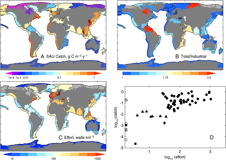
Predominantly coastal large marine ecosystems (LMEs) account for 95% of global fish catch despite covering only 22% of ocean area (Materials and Methods). Fisheries catch per unit area (hereafter referred to simply as “catch”) across LMEs varies by over five orders of magnitude but most produce catches between 0.01 and 1 g C⋅m⁻²⋅y⁻¹. Contributions from small-scale fisheries and discards are largest in the tropics, where increases to between 1.5 and 2 times industrial values are common (Fig. 1B). The lowest catches were in Arctic and Antarctic systems, with Australian LMEs and the insular Pacific-Hawaiian LME also having very low values. Most upwelling systems (e.g., Peru/Chile, Benguela, and Canary) and many temperate and subpolar systems have elevated catch. High catches extend to the tropics in Southeast Asia. Perhaps most striking, however, is that catch in adjacent LMEs (e.g., Northern Australia, Southeast Asia) or between LMEs commonly classified as similar (e.g., Peru/Chile versus California upwelling LMEs) often vary by over an order of magnitude.

Fig. 1.

Catch and effort summary. (A) The average of the top 10 annual catches by LME from the SAU catch reconstruction (6) expressed as grams of carbon per square meter per year. A wet weight-to-carbon conversion of 9:1 was used (3). Catch in the central Arctic is very small (<1e-8 g C⋅m⁻²⋅y⁻¹) and is not shown. The black hatching reflects smaller inland seas and embayments not well resolved by ESM2.6 (see text). The gray hatching corresponds to low-effort, low-catch (LELC) outliers from D. (B) The ratio of the average of the top 10 total to top 10 industrial-only catches. The light gray LMEs in the Arctic correspond to systems with no reported industrial catch. (C) The average of the top 10 effort years expressed as integrated effective vessel power (effective watts per square kilometer) (27). The gray LMEs have no effort data but, due to uncertainties in the location of fishing fleets, may have catches (e.g., Chukchi Sea and Aleutian LMEs). (D) Plot of landings in A versus effort in C. The squares are Arctic and Antarctic LMEs, the triangles are Australian LMEs, and the diamond is the insular-Pacific Hawaiian LME. All other points are shown as circles. The open symbols indicate no effort data. These have been placed along the lower effort bound in D, although lack of data does not necessarily imply low effort.

Maximum fishing effort also varies sharply between LMEs (Fig. 1C). Interpretation of inter-LME effort differences, however, is impeded by large uncertainties in catch per unit of vessel power for different gears, fish targets, and fishing histories (27, 30). In the Peru–Chile upwelling system, for example, an efficient small boat fishery targeting massive aggregations of schooling small pelagic fish has sustained exceptionally high catch rates despite modest vessel power. We thus discarded a nuanced treatment of cross-LME fishing effort differences and instead began our endeavor to unravel drivers of the patchwork of catch variation in Fig. 1A by identifying low-effort, low-catch (LELC) outlier LMEs where catch is less likely to strongly reflect the trophodynamic constraints of primary interest herein (Materials and Methods).

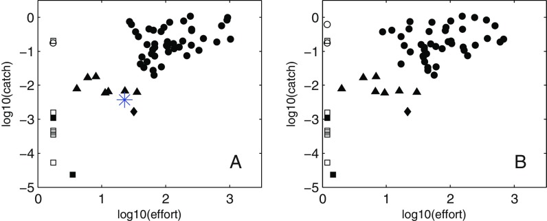
Three effort, catch groupings were readily apparent (Fig. 1D). The first, indicated by squares, included most Arctic systems, where severe weather and ice contribute to extremely low effort and low catch. A second, less marked LELC grouping included Australian LMEs (triangles), where conservative quota-based regulations contribute to high percentages of sustainable fishing within relatively low productivity waters (7, 31, 32), and the oligotrophic insular-Pacific/Hawaiian LME (diamond). The correlation between effort and catch across the remainder of the systems was low (r = 0.34), supporting potentially prominent trophodynamic constraints. Our analysis thus focuses on this final grouping, although sensitivity to including LELC outliers (gray hatched systems in Fig. 1A) will be revisited in Discussion.

Connecting Phytoplankton and Fish.

We considered a sequence of four trophodynamic models of increasing complexity that embody prominent existing hypotheses for trophodynamic controls on fish. Each model was posed in strictly energetic terms—relating catch, a flux in grams of carbon per square meter per year, to an estimate of the energy flux at the characteristic trophic level of the catch. Our intent was to transparently assess the degree to which proposed macroecological patterns embodied in each model are needed to reconcile stark interregional catch differences, while acknowledging the need to further isolate mechanisms underlying those patterns that do.

Model 1 assumes that catch (C) in each LME can be explained by NPP after adjusting for the trophic level of the catch:

$$C=\mathrm{\alpha }\times \text{NPP}\times {\text{TE}}^{\left({\text{TL}}_{\text{eq}}-1\right)}.$$ [1]

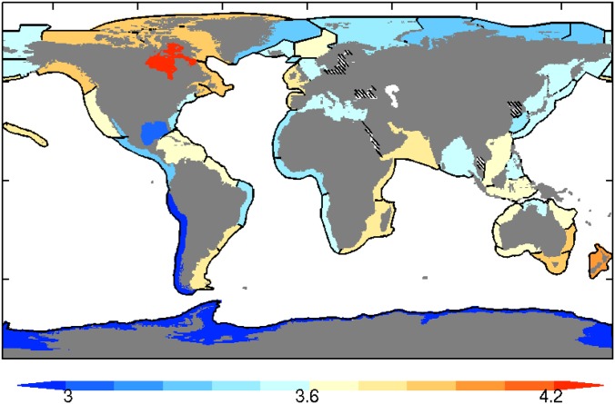
This model is analogous to that used by Pauly and Christensen (3) to calculate the primary production required to sustain fisheries, but here we apply it in reverse to assess how well NPP can explain catch. TL_eq is the equivalent trophic level of the aggregate catch derived from FishBase (33) (Materials and Methods). Phytoplankton are assigned to trophic level 1, such that TL_eq-1 is the number of trophic steps separating phytoplankton from the fish catch. TL_eq generally ranges from minimum values of ∼3 in LMEs where catch is dominated by small pelagic fish (e.g., Peruvian anchovetta) to >4 for LMEs where catch is dominated by larger fish (Fig. S1). The two dimensionless free parameters in model 1 are the trophic transfer efficiency (TE), controlling the decay of energy between trophic levels, and a harvesting factor (α) interpreted as the fraction of energy available at TL_eq that is realized as catch. Single values of TE and α are fit across LMEs such that any interregional variation in these parameters would appear as unexplained catch variance.

Fig. S1.

The equivalent trophic level of the aggregate catch (TL_eq) calculated via Eq. 4 with trophic efficiency, TE = 0.1.

Model 2 tested whether catch is better related to the energy available from the plankton food web via the flux of detritus to the sediment (FDET) and mesozooplankton production not consumed by other zooplankton (MESOZP). It thus replaced NPP in Eq. 1 with energy flows through these benthic and pelagic conduits while keeping the same 2 degrees of freedom (α, TE):

$$C=\mathrm{\alpha }\left(\text{FDET}\times {\text{TE}}^{\left({\text{TL}}_{\text{eq}}-1\right)}+\text{MESOZP}\times {\text{TE}}^{\left({\text{TL}}_{\text{eq}}-2.1\right)}\right).$$ [2]

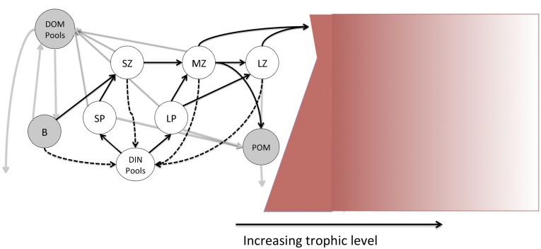
The model is depicted in Fig. S2. FDET and MESOZP in Eq. 2 are referenced to detrital and zooplankton trophic levels assumed in FishBase (1 and 2.1, respectively) to be consistent with TL_eq estimates. We note, however, that Eq. 2 only relies on these values to estimate the number of trophic steps separating plankton food web fluxes and catch. COBALT’s more dynamic representation of plankton food webs (29) is reflected in FDET and MESOZP. We did not attempt to separately model benthic and pelagic catch because fish guilds strongly intermingle in shelf systems where both FDET and MESOZP are significant (15). Benthic primary production, which remains weakly constrained in magnitude, global distribution, and contribution to fish food webs (34, 35), will be addressed in Discussion.

Fig. S2.

A conceptual diagram of the model for the energy exchanges through the planktonic food web to fish adopted herein (see text for description).

Model 3 was analogous to model 2 but considered whether catch is consistent with reduced trophic transfer efficiencies in warm-water tropical and subtropical systems due to high metabolic demands (36, 37). This possibility is parameterized with a dimensionless factor f_T that adjusts TE in Eq. 2 for warm-water systems:

$${\text{TE}}_{\text{warm}}=f_T\text{TE};\hspace{1em}{T}_{100}>T_{100,\text{warm}},$$ [3]

where T₁₀₀ is the 100-m average temperature in each LME, and f_T and T_100,warm are single values fit to catch across LMEs, giving 4 degrees of freedom.

Last, model 4 tested whether different characteristic trophic efficiencies for benthic (TE_B) and pelagic (TE_P) fluxes in Eq. 2 can better explain observed catch. This reflects hypothesized lower foraging costs for benthic environments due to their reduced dimensionality relative to pelagic environments (15). The change was made in addition to the differentiation between warmer and cooler environments reflected in Eq. 3, bringing the number of degrees of freedom to 5. Differentiation of TE_B and TE_P is not meant to imply distinct food chains. Rather, values reflect benthic or pelagic-only limits and their weighting via Eq. 2 provides a means of inferring an emergent TE from catch in mixed benthic/pelagic systems.

Estimates of the physical and planktonic drivers in models 1–4 are drawn from the last 5 y of a 55-y ESM2.6 simulation (Materials and Methods). ESM2.6 robustly captures observed and/or satellite-based/empirically based estimates of physical and biogeochemical properties and fluxes across most LMEs (Table S1). Exceptions are smaller inland seas and shallow coastal embayments (Baltic, Black, Red, and Yellow Seas and the Gulf of Thailand) with intricate exchange flows and strong benthic interactions that remain poorly resolved. These five systems are marked with black hatching in Fig. 1A and have not been considered herein.

Table S1.

ESM2.6 skill assessment

Quantity	r	Bias	RMSE	Notes
SST*	0.997	−0.04	0.87	World Ocean Atlas (75)
SSS*	0.94	−0.21	0.79	World Ocean Atlas (76)
Surface NO3	0.87	−0.15	0.36	World Ocean Atlas (78)
NO3 at 100 m	0.83	−0.02	0.22	World Ocean Atlas (78)
Surface O2*	0.996	−0.13	0.21	World Ocean Atlas (79)
O2 at 100 m*	0.94	+0.11	0.55	World Ocean Atlas (79)
Surface Chl	0.74	−0.23	0.32	SeaWiFS (77)
Surface Chl (>25 m)	0.84	−0.12	0.22	SeaWiFS (77); GEBCO 1-min bathymetry (80)
NPP, VGPM	0.83	−0.10	0.19	Behrenfeld and Falkowski (81)
NPP, Eppley-VGPM	0.87	−0.06	0.15	Behrenfeld and Falkowski (81); Eppley (82)
NPP, (VGPM+Eppley)/2	0.89	−0.08	0.15	Behrenfeld and Falkowski (81); Eppley (82)
Mesozooplankton biomass	0.65	+0.10	0.25	Moriarty and O’Brien (83)
Mesozooplankton production	0.73	+0.09	0.27	Moriarty and O’Brien (83); Hirst and Bunker (84); as described by Stock and Dunne (40)
Export at 100 m	0.77	−0.15	0.23	Dunne et al. (39); Behrenfeld and Falkowski (81)

All quantities not marked with an asterisk (*) were log₁₀ transformed after averaging across each LME to remove positive skew and allow comparison across orders-of-magnitude differences between LMEs.

Models 1–4 were fit to the mean of the top 10 catches using maximum-likelihood estimation assuming a Gaussian error distribution of the residuals of the log₁₀-transformed modeled and observed catch. This assumption was confirmed with a Kolmogorov–Smirnov test. The small sample Akaike information criterion (AIC_c) was used to compare models and Akaike weights (w_AIC) were used to quantify the relative evidence for each model (38). Values of TE were constrained within typical observed ranges of 0–0.4 (3, 11), and α was constrained between 0 and 1.

Trophodynamic Drivers of Global Fish Catch.

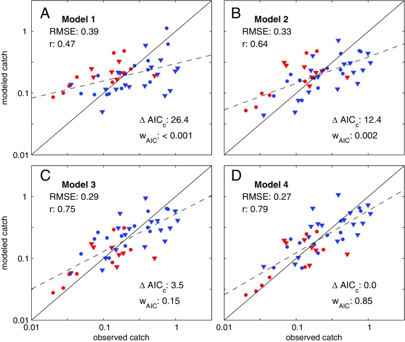
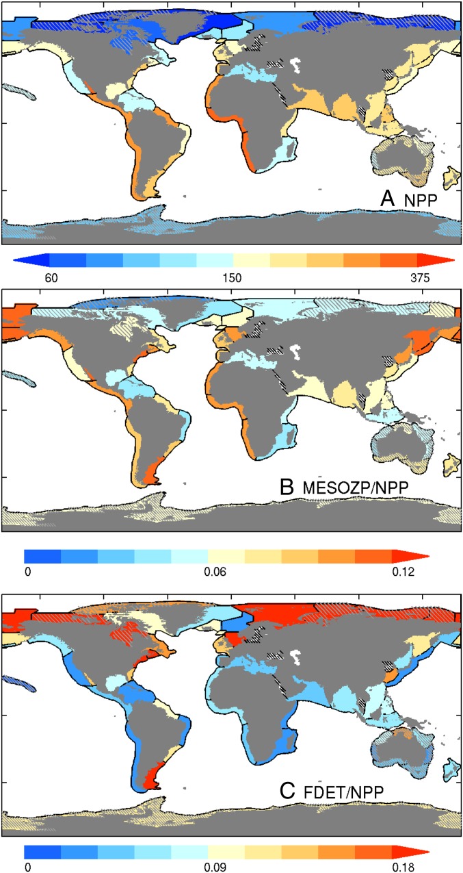
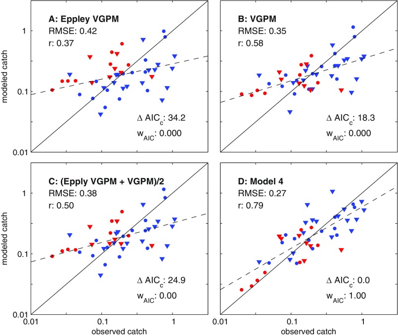
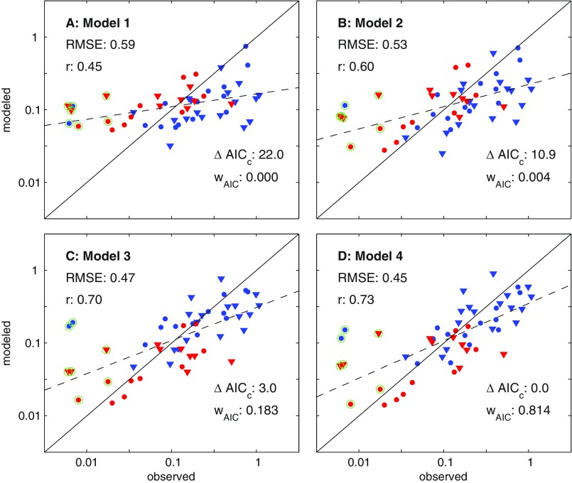
Catch estimates based on NPP (model 1) failed to predict large inter-LME catch differences, markedly overestimating low-catch and underestimating high-catch LMEs (Fig. 2A). This is consistent with Ryther’s contention that NPP differences alone are insufficient to explain cross-ecosystem catch differences. Closer inspection of cross-LME NPP differences (Fig. 3A) provides further insight. With the exception of extremely high/low-latitude Arctic/Antarctic systems, NPP is tightly bounded between 100 and 400 g C⋅m⁻²⋅y⁻¹, far from the two order-of-magnitude catch differences in Fig. 1A. The relative stability of NPP across LMEs reflects the strong feedback between NPP and nutrient recycling (39): as nutrients become scarce, plankton communities shift toward microbial-dominated food webs that efficiently recycle nutrients, buffering NPP declines. Little of this recycled microbial production, however, ever reaches fish because it must traverse multiple often inefficient trophic links to do so (29). The same biases evident in Fig. 2A are found when model 1 is forced with satellite-based NPP estimates (Fig. S4).

Fig. 2.

Comparison of estimated catches from trophodynamic models 1–4 (A–D) with SAU estimates (6). LMEs are divided in four categories. The red symbols have T₁₀₀ > 20 °C and blue for cooler systems. The triangles correspond to systems where the FDET is larger than MESOZP (i.e., more benthic LMEs), and the circles, to more pelagic LMEs (Fig. S3). ΔAIC_C is the difference in the small-sample Akaike information criterion between the best-fit model (model 4) and each alternative; r, the Pearson correlation; RMSE, root-mean-squared error; w_AIC, Akaike weight, interpreted as the likelihood that this model is closest to the true model (38). The solid line is the 1:1 line, and the dashed line is a linear fit through the model estimated catches.

Fig. 3.

Energy flow through the planktonic food web. (A) ESM2.6 simulated NPP by LME in grams of carbon per square meter per year. (B) Mesozooplankton production not consumed by other zooplankton (MESOZP) expressed as a fraction of NPP. (C) The flux of detritus to the benthos (FDET) expressed as a fraction of NPP.

Fig. S4.

A–C are fits resulting from using different satellite-based NPP estimates to drive trophodynamic model 1 instead of NPP from ESM2.6. D shows the optimal model 4 fit. All NPP variants are strongly rejected relative to trophodynamic model 4 and (i) show similar underrepresentation of stark cross-LME catch differences, and (ii) strong tendencies to overestimate catch in warm systems and underestimate catch in cold systems.

Fig. S3.

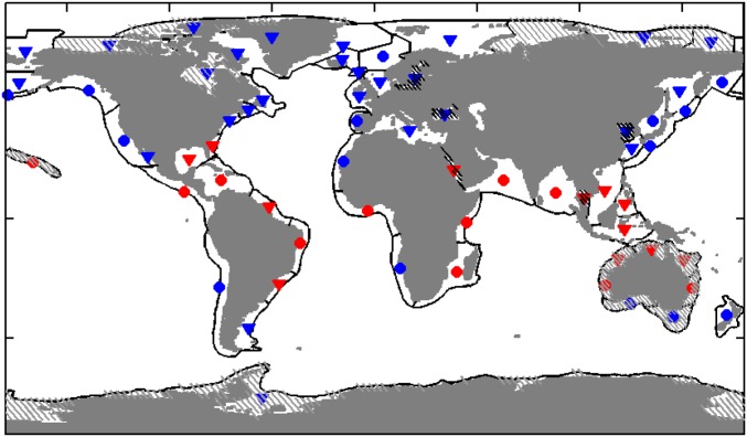
Spatial map of LMEs classified as in Fig. 2. The red points have T₁₀₀ > 20 °C, the blue points have T₁₀₀ < 20 °C, the circles correspond to MESOZP > FDET (more pelagic), and the inverted triangles correspond to MESOZP < FDET (more benthic). We note that classification is sensitive to the offshore extent of LME boundaries, and systems classified as more pelagic may have subregions with energetic benthic food webs. The intent here is only to provide a useful subdivision for interpreting model strengths and weaknesses in the context of this paper. As in the main text, the gray hatching corresponds with LELC outliers. The black hatching corresponds to inland seas and shallow coastal systems that remain poorly resolved by ESM2.6.

Explicitly accounting for benthic (FDET) and pelagic (MESOZP) pathways connecting plankton and fish (model 2) sharpens estimated cross-LME catch gradients, resulting in marked improvement in correlation and root-mean-squared error (RMSE) relative to model 1 (Fig. 2B). MESOZP is highly correlated with NPP (r = 0.91), but its relative variations are amplified: a small percentage of NPP (1–6%) passes through mesozooplankton in low-NPP systems (particularly those forming the borders of or within subtropical gyres), whereas higher percentages (6–12%) are typical in elevated NPP temperate regions (Fig. 3B). The trophic amplification of spatial NPP differences in ESM2.6 reflects mechanisms invoked by Ryther: food chains in more productive and/or temperate bloom regions shorten due to increased herbivory on larger phytoplankton and trophic efficiencies increase as ingestion rates become large relative to consumer basal metabolic costs (29, 40). Cross-LME differences in FDET are also accentuated relative to NPP (Fig. 3C), but NPP and FDET are not strongly correlated (r = 0.49). FDET maps more strongly onto shallow continental shelf systems, particularly temperate LMEs with seasonal phytoplankton blooms that have historically produced some of the highest catches (e.g., the North Sea and Northeast US shelf, blue triangles in Fig. 2).

Although model 2 is clearly better than model 1, it still generally overestimates warm-water and underestimates cold-water LME catch (Fig. 2B, red versus blue). Model 3 addresses this by lowering trophic efficiencies in tropical and subtropical systems (T₁₀₀ > 20 °C, Fig. 2C). The 20 °C isotherm corresponds closely with the boundary between low ratios of O₂ supply to demand for fishes in tropical/subtropical systems and rapidly increasing values in temperate waters (36). Even after this improvement, however, model 3 still underestimates very high catch rates in predominantly benthic cold water systems (blue triangles in Fig. 2C), and many of the largest remaining overestimates correspond to predominantly pelagic systems (circles). Model 4 reduces, but does not entirely remove, this tendency by associating higher trophic efficiencies with benthic-dominated food webs (Fig. 2D). Estimates still fall short of the highest catches, many from shallow shelf systems in the temperate Northern Hemisphere (Discussion), but the overall correlation reaches 0.79 and the discrepancies with reconstructed values generally fall below a factor of 2 (i.e., <0.3 RMSE on a log₁₀ scale) for catch rates per unit area spanning two orders of magnitude across LMEs. The Akaike weights support model 4 (w_AIC = 0.85) as the model closest to the true dynamics. A lesser but nonetheless significant weight is associated with model 3 (0.15). Models 1 and 2 received negligible weights.

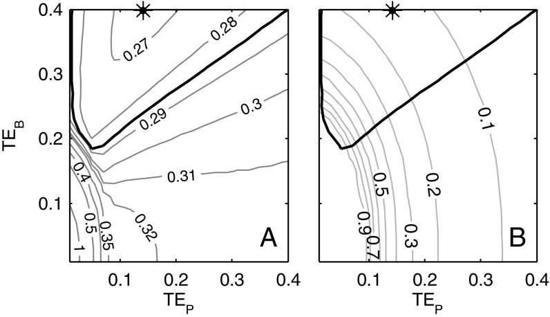
The parameters corresponding to the best-fit case for model 4 infer catch as 14% of available energy (α = 0.14), TEs in tropical/subtropical systems that are 74% of temperate values, and greater benthic than pelagic TEs (TE_B = 0.40, TE_P =0.14). A range of parameter combinations, however, can produce statistically similar results. The inferred ratio of TE for tropical/subtropical waters relative to higher latitude systems (f_T) is robustly less than 1, with 95% f_T confidence intervals covering 0.62–0.86. Model skill was greatest with elevated values for TE_B relative to TE_P, but the gradations in fit between a range of combinations from the high-TE_B, low-TE_P quadrant were modest (Fig. 4A). This holds even if TE values beyond the plausible range of 0–0.4 are allowed.

Fig. 4.

Model 4 parameter uncertainties. (A) Contours of the optimal RMSE for each value of TE_P and TE_B (i.e., the fit reflects an optimization over α, f_T, and T_100,warm for each TE_B, TE_P combination). The gradual slope of the contours across the upper left quadrant of the parameter space and extending into the upper right quadrant indicates weak constraints on TE values across this range. The star corresponds to the best fit in TE_B, TE_P space. The thick black contour corresponds to the 95% confidence interval on TE_B, TE_P. (B) As in A, but the optimal α value for each TE_B, TE_P combination is contoured instead of RMSE. Note the broad range of α values that fall within the 95% TE_B, TE_P confidence intervals and the strong negative correlation between TE values and α.

Perhaps the most significant parameter ambiguity occurred between TE and α (Fig. 4B). Low-TE parameter combinations compensated for reduced energy flows to fish by harvesting a larger fraction of the available energy (i.e., high α), whereas those with higher TEs require only a small harvested fraction. Fig. 4B thus vividly illustrates the need for improved TE constraints to uniquely understand the energetic constraints on catch.

Implications for Future Change.

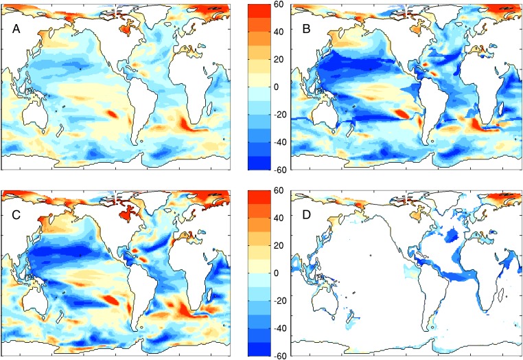
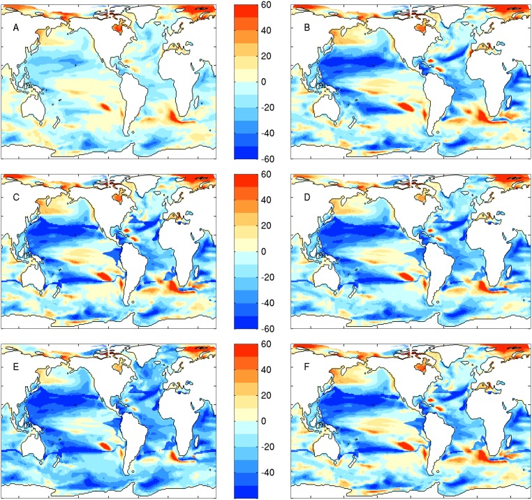
The computational cost of ESM2.6 prevented simulating the many centuries required for climate change projections (41). We could, however, examine the broad-scale trophodynamic implications of climate change using projections from an analog model, ESM2M-COBALT (25) run at the ∼1° horizontal ocean resolution typical for projections used for the Intergovernmental Panel on Climate Change Fifth Assessment Report. Projected percent catch changes in the latter half of the 21st century coincided with, but were considerably larger than, projected percent changes in NPP (Fig. 5 A and B). This amplified pattern holds for the range of parameter values within the 95% confidence interval in Fig. 4, and the optimal parameter settings for models 2 and 3 (Fig. S5). Although regional NPP projections vary between ESMs (42–44), Fig. 5 joins a growing body of evidence for amplified climate change impacts at higher trophic levels (24–26). Projected regional changes in catch may exceed 50%, far above oft-cited modest-to-moderate global NPP trends under climate change (42), and adding urgency to efforts to understand the combination of large-scale and local processes influencing regional climate change impacts on marine resources (45–48).

Fig. 5.

Projected change in NPP and catch under a high-emissions scenario (RCP8.5) from ESM2M-COBALT (25, 69) between 1951–2000 and 2051–2100 using the best-fit trophodynamic model: (A) percent change in NPP, (B) percent change in fish, (C) percent change in MESOZP, and (D) percent change in FDET. FDET changes are only shown for FDET > 2 g C⋅m⁻²⋅y⁻¹ to emphasize changes in systems with significant benthic relative to pelagic fluxes.

Fig. S5.

Comparison of projected percent changes in catch from a range of fish catch models. Differences are between means over the latter half of the 21st century (2051–2100) relative to the latter half of the 20th century (1951–2000). (A) Projected percent change in catch for the best-fit trophodynamic model 1 (i.e., NPP-only model). This model produces much smaller changes in catch but was firmly rejected in favor of alternative models (Fig. 2). (B) Projected catch change for the best-fit trophodynamic model 2. Note the amplification relative to A from accounting for plankton food web dynamics. (C) Projected catch change for the best-fit trophodynamic model 3. (D) Projected catch change for the best fit trophodynamic model 4. (E) Projected change for a “low TE_P” parameter setting (TE_P = 0.05, TE_B = 0.4) that remains statistically indistinguishable from the best case in D. (F) Projected change for a “low TE_B” parameter setting (TE_B = 0.20) that remains statistically indistinguishable from the best case in D. Note the robust nature of amplified catch differences for all trophodynamic models except the strongly rejected trophodynamic model 1.

The same trophodynamic mechanisms operating on spatial NPP gradients to sharpen inter-LME catch differences in the contemporary ocean steepened NPP trends under climate change. NPP declines were “triple taxed” for MESOZP (25) (Fig. 5C): zooplankton consumed less, a smaller fraction of what they consumed was left for growth and reproduction after meeting basal metabolic costs, and they were forced to rely more on secondary production as large phytoplankton were suppressed by nutrient declines associated with increasing stratification (i.e., mesozooplankton trophic level increases). MESOZP in areas of increasing NPP generally benefited from the reverse of these processes. Meanwhile, the detrital flux to the benthos (Fig. 5D) in most low and mid-latitude nutrient-limited regions was tightly tied to declining nutrient fluxes to the euphotic zone as stratification increases. Declines were exacerbated by shallower remineralization of sinking detritus in acidifying waters due to reduced protection of organic matter by calcite and aragonite minerals (49, 50).

The effect of reduced trophic efficiencies in tropical waters (f_T < 1 for T₁₀₀ > 20 °C) was reflected in regions of discontinuous deepening of projected catch reductions or damping of catch increases where waters crossed the 20 °C temperature isotherm as the ocean warms (Fig. 5B). Although steep increases in the ratio of oxygen supply to demand in the vicinity of this isotherm support a sharpen response (36), it is likely overaccentuated by the binary representation of this effect used herein.

We note that the projections in Fig. 5 reflect only the trophodynamic contribution to projected catch. The results implicitly assume that fish will occupy novel warm environments expected in equatorial waters (51) to the extent that trophodynamic considerations allow. This contrasts with the bioclimate envelope approach for modeling fisheries, which draws finer gradations in habitat suitability based on present species range and projects downward catch trends in novel equatorial environment (52). Integration of trophodynamic insights herein with refined habitat and adaptability considerations is needed to reduce uncertainty in equatorial catch projections.

Discussion

Revisiting the trophodynamic drivers of fish catch with new datasets and models showed that a considerable fraction of variation in maximum catch across globally distributed ecosystems can be explained by planktonic food web and trophic transfer considerations. NPP, however, was clearly inadequate to explain stark interregional catch differences. Furthermore, the trophodynamic factors required to reconcile catch differences in the contemporary ocean robustly amplified catch trends expected under climate change, such that projected changes by the end of the 21st century may exceed 50% in some regions under high emissions. This underscores the need for ecosystem-based fisheries management strategies that are resilient to potentially large changes in catch potential, and the need for improved constraints on regional ocean productivity trends. Although ESM2.6 provides an effective global perspective of cross-LME catch patterns and their sensitivity to change, understanding of specific regions may be most rapidly achieved by combining improving global projections and downscaling with high-resolution regional models (46–48).

Interregional catch variations left unexplained by the trophodynamic processes considered herein may reflect unresolved effects of past and present fishing effort, persistent uncertainties in catch reconstructions, errors in planktonic food web estimates, and unresolved trophodynamic factors. We discuss each of these elements before revisiting Ryther’s hypothesis.

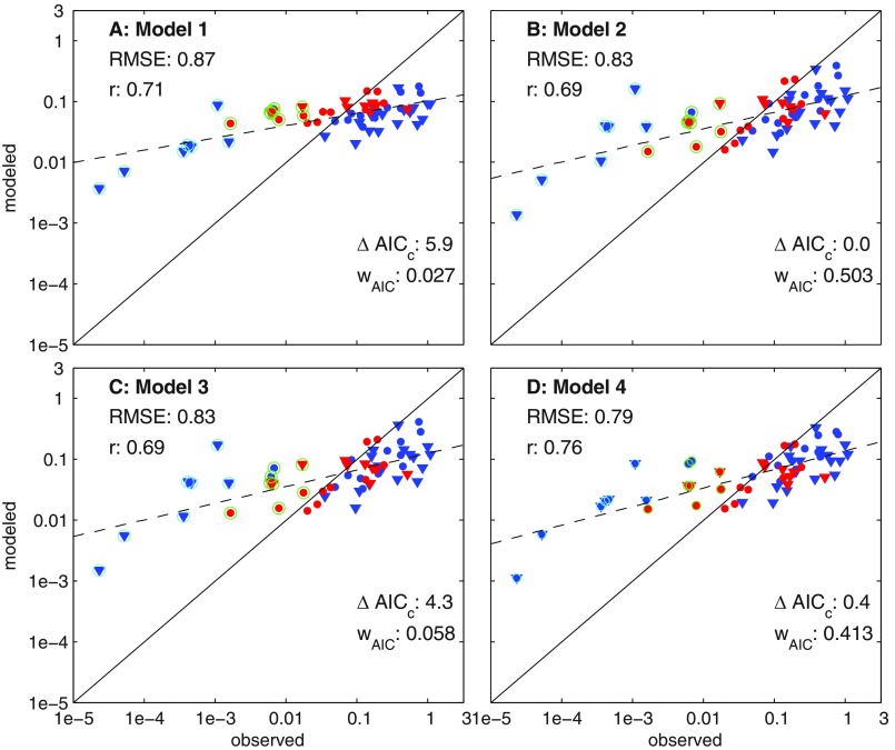
Fishing effort was coarsely handled by identifying and filtering out LELC outlier LMEs as systems where catch was less likely to reflect trophodynamic constraints (Fig. 1D). Adding back the Australian and Hawaiian systems moderately degrades trophodynamic model skill (Fig. S6, r = 0.73, RMSE = 0.45) and produces a strong negative correlation between inter-LME effort differences and unexplained catch variability (r = −0.53 versus r = −0.27 without these systems). The inferred trophodynamics, however, remain similar. If Arctic/Antarctic LELC outliers are included, estimates from all trophodynamic models are highly correlated with catch, but all egregiously overestimate Arctic/Antarctic catches and egregiously underestimate catch in other systems (Fig. S7, RMSE = 0.75). Arctic/Antarctic catches simply cannot be reconciled with other LMEs via trophodynamic factors alone, and including these systems in model fitting risks strong aliasing of effort effects onto trophodynamic estimates, and gives a misleading impression of the value of NPP as a predictor of cross-LME catch differences.

Fig. S6.

Fits for models 1–4 (A–D) after adding back the Australian and Hawaiian LMEs. Catches in these systems (outlined with green circles) are generally strongly overestimated by the model. This increases the RMSE and decreases the correlation for most models, but the fit still improves significantly with each model iteration and the best solution has the same properties of the fit without these systems: depressed TEs in tropical systems and elevated TEs associated with benthic fluxes (without Australia/Hawaii: α = 0.14, TE_P = 0.14, TE_B = 0.40, f_T = 0.73, T_100,warm = 20 °C; with Australia/Hawaii: α = 0.19, TE_P = 0.10, TE_B = 0.33, f_T = 0.66, T_100,warm = 20 °C).

Fig. S7.

Fits for models 1–4 (A–D), but adding back both the Australian/Hawaiian and Arctic/Antarctic LELC outliers. Australian systems are again circled in green and Arctic systems in light blue. Note the large increase in the range of catches with the introduction of the extremely lightly fished Arctic systems. As described in the main text, all models show high correlation, but this correlation masked large, systematic overestimation of catch in Arctic/Antarctic systems and stark underestimation of most other systems.

We note that the low correlation between inter-LME effort differences and remaining misfits after filtering out LELC outliers (r = −0.27) does not rule out effort from contributing to remaining misfits. The peak integrated vessel power measure applied herein does not account for differences in catchability (27), profitability (53), and time integrated fishing impacts (7) that can further influence realized catches.

Accounting for small-scale fisheries alters catch patterns relative to past studies of oceanographic controls on fish catch (6). We assessed the trophodynamic implications of this by refitting models to industrial-only catch data commonly reported to the Food and Agriculture Organization (FAO). Overall model skill contrasts were similar (Table S2), but fitting to industrial-only catch inferred somewhat lower TEs in tropical systems (f_T = 0.68 versus f_T = 0.73) to explain reduced catch estimates where small-scale fisheries are most prominent. Improvements in catch reporting (6) could further reduce biases in trophodynamic estimates arising from catch reporting gaps. We also note that the catch-based analysis herein cannot address potential yield of largely unexploited but potentially substantial mesopelagic fisheries (12).

Table S2.

Additional sensitivity tests for trophodynamic model inference

Model simulation	Model 1 (r/RMSE/wAIC)	Model 2 (r/RMSE/wAIC)	Model 3 (r/RMSE/wAIC)	Model 4 (r/RMSE/wAIC)
Baseline*	0.466/0.388/0.000	0.644/0.332/0.002	0.755/0.286/0.151	0.791/0.267/0.848
Top 5 catch years	0.485/0.383/0.000	0.652/0.328/0.002	0.761/0.281/0.141	0.798/0.263/0.858
Top 20 catch years	0.446/0.393/0.000	0.640/0.333/0.002	0.750/0.288/0.156	0.787/0.269/0.841
All 61 catch years	0.447/0.387/0.000	0.633/0.332/0.002	0.749/0.285/0.233	0.780/0.270/0.764
ESM2.6 years 41–45	0.466/0.388/0.000	0.644/0.332/0.002	0.753/0.286/0.122	0.792/0.266/0.876
ESM2.6 years 46–50	0.466/0.388/0.000	0.645/0.332/0.003	0.747/0.290/0.117	0.787/0.269/0.880
ESM2.6 years 46–55	0.466/0.388/0.000	0.645/0.332/0.002	0.751/0.288/0.133	0.790/0.268/0.865
ESM2.6 years 41–55	0.466/0.388/0.000	0.645/0.332/0.002	0.752/0.287/0.130	0.791/0.267/0.868
$\overline{\mathrm{TE}}$ from 1 to 4.5	0.466/0.388/0.000	0.643/0.333/0.002	0.755/0.286/0.145	0.791/0.267/0.854
$\overline{\mathrm{TE}}$ from 1 to 5	0.466/0.388/0.000	0.642/0.333/0.001	0.755/0.286/0.139	0.792/0.267/0.859
0.5 benthic NPP	0.466/0.388/0.000	0.637/0.335/0.002	0.758/0.284/0.297	0.783/0.271/0.701
3.0 benthic NPP	0.466/0.388/0.000	0.603/0.349/0.001	0.758/0.283/0.773	0.759/0.283/0.226

Rows are sensitivities, whereas columns provide skill metrics for each model (r, Pearson correlation; RMSE, root-mean-squared error; w_AIC, the Akaike weight). The baseline is the simulation used in the main text (i.e., averaging the top 10 catch years, forcing from years 51–55 of the ESM2.6 simulation, $\overline{\mathrm{TE}}$ in Eq. 5 based on energy transfer through trophic levels 1–4). The “catch year” sensitivities refer to fitting to catch averaged over fewer or more years. The “ESM2.6” sensitivities refer to using plankton food webs from different segments of the ESM2.6 simulation to fit the trophodynamic models. The $\overline{\mathrm{TE}}$ sensitivities consider the effect of estimating $\overline{\mathrm{TE}}$ based on energy transfer through trophic levels 1–4.5 or 1–5. The benthic NPP sensitivities consider possible transfers of 0.5 and 3 Pg C⋅y⁻¹ to fish food webs globally (distributed across areas <50 m deep). The best model, according to the Akaike weights, is bolded.

^*Used in paper.

We limited our analysis of ocean productivity constraints of fish catch to LMEs due to their overall predominance in the global fish catch (Materials and Methods, 95% of catch despite 22% of ocean area). High-seas fisheries also target many highly migratory species (54), making the spatial associations with ocean productivity required for this study difficult. Although fishing has expanded offshore in recent decades, degrading a number of high value stocks (54), catch outside LMEs remains below 9% of the global total in all years. Offshore effort and ecosystem-level exploitation per area also generally remains far less than in coastal regions (55, 56). This is in part a reflection of the high capital cost of high-seas fishing that restricts this activity to a select subset of nations (57). Plotting the integrated catch and effort firmly places non-LME regions among the LELC outliers in Fig. 1D (Fig. S8).

Fig. S8.

Comparison of effort versus catch using (A) the mean of the top 10 catch and effort years, calculated independently; and (B) the mean of the top 10 catch years and the mean of the top 10 corresponding effort years. In the latter case, we had to restrict the catch time series to 1950–2006. The LELC clusters are unaffected by these variants in approach. The blue asterisk in A corresponds to the integrated effort/catch values for all regions outside the LMEs. The LELC combination is consistent with these regions accounting for only ∼5% of global catch despite accounting for 78% of ocean area.

For the plankton food web, we relied on ESM2.6 to resolve two primary contrasts between NPP and the supply of energy to fish. The first was the amplification of cross-LME percent differences in mesozooplankton production relative to NPP (Fig. 3B). The second was similarly marked variation in the detrital flux to the benthos combined with a strong skew in FDET toward LMEs with broad, shallow shelves (Fig. 3C). Both of these patterns are supported by past empirical analysis and understanding of the underlying mechanisms (29, 40, 58, 59). However, although the performance of ESM2.6 at the LME scale was encouraging (Table S1), the model still suffers from regional biases and incomplete process resolution. Perhaps most notable for this are the 40-m minimum depth (Materials and Methods) and stubborn ESM2.6 low-chlorophyll biases in very high-chlorophyll near-shore regions. Improvement is needed, but the robustness of conclusions when using satellite NPP estimates that do not suffer from these biases bolsters confidence in our primary conclusions (Fig. S4).

Our trophodynamic models did not consider the potential contribution of benthic primary producers because the magnitude of benthic NPP, its spatial distribution, and how much it contributes to local fish food webs remain highly uncertain (34, 35). Macrophytes, the dominant benthic primary producer in coastal systems, were recently estimated to provide 1.5 Pg C⋅y⁻¹ (σ = 0.73 Pg C⋅y⁻¹), or about 3% of global NPP. Approximately 43% of this production is exported from the regions in which it grows (34, 35). Macrophyte production may be augmented by ∼1 Pg C⋅y⁻¹ sea grass, mangroves, corals, and marsh plants with similarly uncertain contributions to food webs (60). To test the sensitivity of our results to inclusion of benthic NPP, we considered bounding scenarios where 0.5 and 3 Pg C⋅y⁻¹ of benthic NPP was distributed evenly across waters <50 m deep and added this production to FDET in Eq. 2. A global contribution of 0.5 Pg C⋅y⁻¹ to local fish food webs had little effect, but 3 Pg C⋅y⁻¹ eroded the value of invoking elevated trophic efficiencies for benthic systems and favored model 3 over model 4 (Table S2). Improved benthic NPP constraints are needed, but the large skill differences between trophodynamic models 3–4 and models 1–2 are robust, as is the amplification of catch trends under climate change (Fig. S5).

Improved TE constraints were found to be critical for reducing the scope of similarly performing parameter contributions and quantifying the fraction of available energy realized as catch (Fig. 4B). This finding is consistent with other studies (11–13), suggesting the importance of moving from the broad TE ranges applied herein toward estimation of TE probability densities (61). Such probability densities could allow Bayesian approaches to more formally incorporate prior parameter estimates.

The blending of empiricism and mechanistic principles applied in this study is intended to help bridge the gap between predominantly data-driven analysis of catch indicators (14, 15, 19) and the development and application of more mechanistic global fisheries models rooted in theoretical constraints but of often challenging complexity (13, 62–65). Parameters and emergent patterns from the simple trophodynamic models herein can be directly compared against simulated patterns from these latter models. The simple trophodynamic approach has also enabled rapid exploration of parameter space for alternative parameter combinations that can explain observed catch patterns equally well. Although we cannot fully resolve the detailed mechanisms that may underlie, for example, reduced trophic efficiencies inferred in tropical systems or enhanced trophic efficiencies in benthic-predominant systems, we have demonstrated their potential prominence in determining large-scale catch patterns.

The new datasets and models applied herein have allowed a richer examination of the range of trophodynamic processes required to reconcile pronounced gradients in fish catch across disparate ecosystems. Results invoke dynamic variations in the length and efficiency of food chains along productivity gradients analogous to those discussed by Ryther, although contrasts between systems are less stark than Ryther invoked. They also stress the importance of shallow benthic environments and metabolic contrasts between tropical and other systems. Although these refinements are notable, the essence of Ryther’s hypothesis, that NPP and trophodynamic processes must act synergistically to generate stark observed catch gradients, is supported by our results. So too is the corollary that NPP alone is a poor indicator of differences in fish yields across disparate marine ecosystem types (1, 15). Neglecting the trophodynamic processes required to reconcile catch across these regions risks severely underestimating cross-LME differences in maximum sustainable catch in the contemporary ocean, and underestimating potential trends under climate change.

Materials and Methods

The trophodynamic catch models described in the main text require estimates of fish catch, catch trophic level, fishing effort, and plankton food web fluxes. Catch was obtained for each LME from the SAU project (www.seaaroundus.org) for the years 1950–2010. Catches in metric tons of wet weight per year for each LME were converted to grams of carbon per square meter per year using a 1/9 ratio of carbon to wet weight (3). The mean of the top 10 annual total catches was used for fitting the trophodynamic models described in the main text. This choice reflects a compromise between including enough years to average out the effect of highly unsustainable fishing, while not requiring so many years that catch estimates reflect long periods before industrialized fishing when catch was less likely to reflect ocean productivity constraints. Results, however, were robust to averages taken over 5, 10, 20 y, or even the 60 y (Table S2).

We focus on catch in LMEs. These are ecologically linked mainly coastal systems (66) that have been broadly adopted for ecosystem-based management and past studies of global fish catch (7, 13–15, 19). LMEs account for 95% of fish catch in the SAU reconstruction, despite covering only 22% of ocean area. Further examination of this limitation can be found in Discussion.

Trophic-level data were drawn from FishBase, which derives estimates based on extensive gut content information (33). The equivalent trophic level (TL_eq) of the aggregate catch for each LME was calculated such that the primary production required to support the total catch at TL_eq (right-hand side of Eq. 4 below) was equal to the primary production required based on summing the individual catch constituents (left-hand side):

$${\displaystyle \sum }_{i=1}^m\left(C_i\times {\left(\frac{1}{\overline{\mathrm{TE}}}\right)}^{\mathrm{T}{\mathrm{L}}_i-1}\right)=\left({\displaystyle \sum }_{i=1}^m{C}_i\right)\times {\left(\frac{1}{\overline{\mathrm{TE}}}\right)}^{\mathrm{T}{\mathrm{L}}_{\mathrm{eq}}-1},$$ [4]

where m is the number of species caught in each LME. TL_eq is thus based on matching the implied energetic cost of the disaggregated catch, unlike a biomass weighted average. Although a single fish food web TE is fit for each LME (see main text), the TE between NPP and MESOZP for models 2–4 is calculated by ESM2.6. We thus define $\overline{\mathrm{TE}}$ based on the average decay of energy between TL = 1 and TL = 4 (i.e., piscivores):

$$\overline{\mathrm{TE}}={\left(\frac{\text{FDET}\times {\text{TE}}^{(4-1)}+\text{MESOZP}\times {\text{TE}}^{(4-2.1)}}{NPP}\right)}^{1/3}.$$ [5]

The numerator of Eq. 5 is the energy available at TL = 4, the denominator is the energy at TL = 1, and the 1/3 exponent extracts the mean decay across 3 trophic levels. MESOZP is treated as trophic level 2.1 based on FishBase conventions (33). $\overline{\text{TE}}$ and TL_eq are calculated as TEs for each catch model are estimated, resulting in consistent optimal sets of $\overline{\text{TE}}$, TL_eq, and TE for each model. Results are highly robust to estimating $\overline{\text{TE}}$ across 4, 4.5, and 5 trophic levels (Table S2).

Fishing effort data were mapped from FAO, European, and associated bodies’ data between 1950 and 2006 (30). The mean of the top 10 effective effort years was used in Fig. 1 C and D to broadly characterize cross-LME differences for the purpose of identifying LELC outlier systems (see main text). The same LELC outlier systems are identified if effort years were chosen to precisely match the top 10 catch years (Fig. S8), but this would have prevented use of the last 4 y of the catch time series (2007–2010) that are pending updates to the effort database.

ESM2.6 combines the high-resolution physical climate of GFDL’s CM2.6 global climate model (28), featuring 10-km horizontal ocean resolution and 50-km horizontal atmospheric resolution with the 33 tracer COBALT planktonic ecosystem model (29). The ocean has 50 vertical layers, with 10-m vertical resolution over the top 200 m and a minimum depth of 40 m (i.e., all waters <40 m are treated as 40 m deep). This effects 3.5% of the global ocean and, on average, 12% of the area of LMEs in Fig. 2. ESM2.6 was run for 55 y as a fully coupled ocean–atmosphere–land–sea ice configuration with 1990 greenhouse gas conditions on NOAA’s Gaea supercomputer. The run was initialized with hydrography from year 141 of a 1990 control with the CM2.6 physical climate model and nutrients from the World Ocean Atlas (67), dissolved organic carbon from GLODAP (68), and other fields from a coarse-resolution COBALT simulation (29). The simulation used 15,744 processors for a throughput of ∼0.5 y per d. This is ∼7,500 times the cost per simulation year as GFDL’s ESMs contributed to the Fifth Assessment Report that featured resolutions more typical for climate change simulations (e.g., ∼1–2° oceans and atmospheres) (69).

COBALT’s planktonic food web dynamics are represented with a size-structured nutrient–phytoplankton–zooplankton formulation that draws heavily from allometric constraints to represent plankton physiology and consumer–prey interactions (29). There are three phytoplankton groups (small, large, diazotrophs), three zooplankton groups, free-living bacteria, sinking detritus, and three types of dissolved organic material with differing labilities. Fig. S2 provides a schematic of the plankton food web dynamics most relevant to results herein. Mesozooplankton production is calculated as the sum of medium and large zooplankton spanning size classes between 200 μm and 2 cm in equivalent spherical diameter. We then subtract out consumption of medium zooplankton by large zooplankton. Detritus sinking and remineralization followed a “mineral ballast model” (49, 50), with purely organic detritus having an e-folding remineralization depth scale of 188 m, but this rate is slowed considerably by minerals (e.g., silica, calcium carbonate) and low-oxygen environments. Two perturbations relative to the baseline COBALT formulation (29) were implemented for ESM2.6. First, nitrogen-to-phosphorous ratios of small phytoplankton were elevated and ratios for large phytoplankton lowered for consistency with observed stoichiometric tendencies (70, 71). Second, phytoplankton aggregation was suppressed when nutrients are not strongly limiting (72).

ESM2.6 resolves prominent modes of climate variability, but, like other coupled atmosphere–ocean simulations, the variability does not occur in phase with historical observations (41). Results were not sensitive to using a range of different 5 y or longer averaging periods (Table S2).

Global simulations with COBALT at coarser horizontal resolutions (∼1° latitude, longitude) have been shown to produce quantitatively credible estimates of carbon and energy flow throughout the planktonic food web across broadly defined ocean biomes (29). We extended this evaluation to LME scales for this study (Table S1). ESM2.6 captured broad-scale differences across most LMEs but remained limited in its representation of smaller inland seas and embayments (Red, Yellow, Black, and Baltic Seas, Gulf of Thailand). The primary shortcomings of the model are (i) it underpredicts very high chlorophyll (>5 mg⋅m⁻³) inferred from satellites in near-shore regions (<25 m) and (ii) the fully coupled construction of the model leaves it more susceptible to regional biases and drifts in biome boundaries. Chlorophyll mismatches in near-coastal regions may in part arise from errors in satellite estimates linked to the complex optical properties of these waters (73, 74), but likely also reflect ESM2.6 limitations in near-shore regions—including the 40-m minimum depth and simple representation of sediment/nutrient interactions (29).

Fig. S1 shows the equivalent trophic level of the aggregate catch (TL_eq) from the top 10 catch years calculated with a trophic efficiency (TE) of 0.10 and trophic levels defined by FishBase (33). TL_eq varies by more than a full trophic level across LMEs, ranging from lows of ∼3 for systems where catch is dominated by small pelagic fish (e.g., Peruvian Anchoveta in the Humboldt Current system off Peru) to over 4 for systems targeting larger fish. With TE = 0.1, energy flux considerations alone would thus lead one to expect ∼10 times more catch for systems near the low TL_eq limit in Fig. S1 than near its upper bound.

Fig. S2 shows a schematic of the trophodynamic model reflected in Eq. 2. The left-hand side is a distillation of COBALT's plankton food web. Complete details can be found in Stock et al. (29). Dissolved inorganic nutrients (DIN) are taken up by small and large phytoplankton (SP and LP) that are consumed by small, medium and large zooplankton via size-structured consumer-resource links. Small zooplankton (SZ) are effectively microzooplankton <200 μm in equivalent spherical diameter (ESD), medium zooplankton (MZ) are small to medium-bodied copepods (∼0.2–2 mm ESD), and large zooplankton (LZ) are large copepods and euphausiids (∼0.2–2 cm ESD). Sinking particulate organic material (POM) is generated by phytoplankton aggregation and egested mesozooplankton fecal pellets. Phytoplankton exudates and egestion by smaller zooplankton provide dissolved organic matter (DOM) cycled by free-living bacteria (B) within a microbial loop. Dashed lines indicate energy losses due to respiration and the associated remineralization of nutrients. Mesozooplankton production that is not consumed by other mesozooplankton (MESOZP) and the flux of POM to the benthos (FDET) fuel the fish food web.

The shaded red box at the right of Fig. S2 reflects the flow of energy through the fish food web and its attenuation at higher trophic levels. Three primary assumptions are reflected in the figure. The first is that energy from POM reaching the benthos (FDET) enters the fish food web at a lower trophic level (TL = 1) than MESOZP (TL = 2.1, trophic levels increasing from left to right). Second, we assume that energy from MESOZP and the benthic flux is rapidly distributed across benthic and pelagic environments in shallow systems for which both fluxes are important. This is assumed to be mediated by the numerous species that periodically occupy benthic and pelagic environments (15). The intermingled fluxes then decay at a rate defined by TE, as reflected in the lightening shading from left to right. Lower TE would strengthen the decay of the energy flux across trophic levels and higher TEs would damp it.

Outputs from ESM2.6 were compared against a range of physical and biogeochemical metrics at the LME scale (Table S1). As described in the main text, the skill metrics below omit smaller inland seas (Baltic, Red, Black) and shallow coastal embayments (Gulf of Thailand and Yellow Sea), which remain poorly resolved by ESM2.6.

Physical properties [sea surface temperature (SST), sea surface salinity (SSS)] exhibited a close match to observed values (r > 0.9) from the World Ocean Atlas (75, 76). This high skill was largely maintained for nitrate and oxygen (78, 79). We compared model outputs to sea-viewing wide field-of-view sensor (SeaWiFS) chlorophyll concentration from the years 1998–2007. These years were selected because beginning in 2008 SeaWiFS began to experience outages in coverage lasting up to 96 d. We used the standard, level 3 SeaWiFS chlorophyll a product, which was processed with the OC4 algorithm and had a 9-km and 8-d resolution (77). The correlation against surface chlorophyll was 0.74, with ESM2.6 generally underestimating observed values (bias = −0.23 log₁₀ units, or an ∼40% low bias). Much of this low bias, however, is due to ESM2.6’s failure to capture limited very high chlorophyll values (greater than ∼5 mg Chl⋅m⁻³) in very shallow waters. Bias is greatly reduced when only waters with depths >25 m are considered (−0.12 log₁₀ units or about a 25% low bias, r = 0.84). The underrepresentation of high chlorophyll peaks in shallow regions likely reflects a combination of ESM2.6’s limited resolution of the physical and biological processes in very shallow coastal regions and uncertainties in the contribution of colored dissolved organic matter to satellite-based chlorophyll estimates in the regions (74).

We compared ESM2.6 NPP with two satellite-based NPP algorithms—VGPM and Eppley–VGPM (81, 82) obtained from Oregon State University’s Ocean Productivity website (www.science.oregonstate.edu/ocean.productivity/). These algorithms are representative of the two major variants of latitudinal NPP variations among satellite-based NPP estimates (8), with the original VGPM positing a peak in characteristic photosynthetic rates at moderate temperatures and Eppley–VGPM positing a monotonic increase in rates with increasing temperature. We also considered the mean of the two algorithms. We limited comparisons to those regions where the bottom depth was greater than the euphotic zone depth presumed by the satellite algorithm. ESM2.6 was most consistent with the mean of the two satellite-based algorithms across LMEs, but maintained high correlation and minimal bias against all variants. Fitting trophodynamic model 1 to catch using NPP from ESM2.6 or that from satellite algorithms yielded similar results (Fig. S4).

Mesozooplankton biomass and production was compared against biomass fields from NOAA’s COPEPOD database (83) (www.st.nmfs.noaa.gov/copepod/). A seasonal climatology from ESM2.6 was compared with observed estimates of mesozooplankton carbon mapped on a 1/4 degree grid. COPEPOD estimates for the Hawaiian-Insular Pacific LME were replaced with values from repeat ocean measurements from the Hawaii Ocean time series that used 200-μm mesh nets more suited to subtropical gyre environments (85). Observed and modeled point estimates were then averaged across each LME. We considered only those LMEs with >50 mesozooplankton biomass estimates across all grid points in the LME and all seasons. Estimates of mesozooplankton production were derived using the empirical estimates of mesozooplankton growth provided by Hirst and Bunker (84) as described by Stock and Dunne (40). The resulting correlation with mesozooplankton biomass and production is lower than for NPP and the model is biased about 25% high, but correlations remain >0.6 despite the patchiness of sampling and mesozooplankton biomass fields. A modest high bias is also understandable given incomplete sampling of MZ and LZ biomass by the 350-μm nets used for the vast majority of data within the COPEPOD database (83).

We compared export from the euphotic zone in ESM2.6 with estimates based on the empirical relationship between NPP, SST, and export at the base of the euphotic zone described by Dunne et al. (39), with remotely sensed data again taken from Oregon State’s Ocean Productivity website as described for NPP. Fluxes were adjusted to a common depth of 100 m or the ocean bottom using a near-surface remineralization e-folding scale of 188 m. The export flux from ESM2.6 has a ∼30% low bias relative to Dunne et al. (39) but lies well within the range of global export flux estimates (86).

References

- 1.Ryther JH. Photosynthesis and fish production in the sea. Science. 1969;166(3901):72–76. doi: 10.1126/science.166.3901.72. [DOI] [PubMed] [Google Scholar]
- 2.Lindeman RL. The trophic-dynamic aspect of ecology. Ecology. 1942;23(4):399–417. [Google Scholar]
- 3.Pauly D, Christensen V. Primary production required to sustain global fisheries. Nature. 1995;374(6519):255–257. [Google Scholar]
- 4.Libralato S, Pranovi F, Stergiou KI, Link JS. Trophodynamics in marine ecology: 70 years after Lindeman. Mar Ecol Prog Ser. 2014;512:1–7. [Google Scholar]
- 5.Coll M, Libralato S, Tudela S, Palomera I, Pranovi F. Ecosystem overfishing in the ocean. PLoS One. 2008;3(12):e3881. doi: 10.1371/journal.pone.0003881. [DOI] [PMC free article] [PubMed] [Google Scholar]
- 6.Pauly D, Zeller D. Catch reconstructions reveal that global marine fisheries catches are higher than reported and declining. Nat Commun. 2016;7:10244. doi: 10.1038/ncomms10244. [DOI] [PMC free article] [PubMed] [Google Scholar]
- 7.Mcowen CJ, Cheung WW, Rykaczewski RR, Watson RA, Wood LJ. Is fisheries production within large marine ecosystems determined by bottom‐up or top‐down forcing? Fish Fish. 2015;16(4):623–632. [Google Scholar]
- 8.Carr M-E, et al. A comparison of global estimates of marine primary production from ocean color. Deep Sea Res Part II Top Stud Oceanogr. 2006;53(5):741–770. [Google Scholar]
- 9.Branch TA, et al. The trophic fingerprint of marine fisheries. Nature. 2010;468(7322):431–435. doi: 10.1038/nature09528. [DOI] [PubMed] [Google Scholar]
- 10.Jennings S, van der Molen J. Trophic levels of marine consumers from nitrogen stable isotope analysis: Estimation and uncertainty. ICES J Mar Sci. 2015;72(8):2289–2300. [Google Scholar]
- 11.Libralato S, Coll M, Tudela S, Palomera I, Pranovi F. Novel index for quantification of ecosystem effects of fishing as removal of secondary production. Mar Ecol Prog Ser. 2008;355:107–129. [Google Scholar]
- 12.Irigoien X, et al. Large mesopelagic fishes biomass and trophic efficiency in the open ocean. Nat Commun. 2014;5:3271. doi: 10.1038/ncomms4271. [DOI] [PMC free article] [PubMed] [Google Scholar]
- 13.Jennings S, Collingridge K. Predicting consumer biomass, size-structure, production, catch potential, responses to fishing and associated uncertainties in the world’s marine ecosystems. PLoS One. 2015;10(7):e0133794. doi: 10.1371/journal.pone.0133794. [DOI] [PMC free article] [PubMed] [Google Scholar]
- 14.Conti L, Scardi M. Fisheries yield and primary productivity in large marine ecosystems. Mar Ecol Prog Ser. 2010;410:233–244. [Google Scholar]
- 15.Friedland KD, et al. Pathways between primary production and fisheries yields of large marine ecosystems. PLoS One. 2012;7(1):e28945. doi: 10.1371/journal.pone.0028945. [DOI] [PMC free article] [PubMed] [Google Scholar]
- 16.Ware DM, Thomson RE. Bottom-up ecosystem trophic dynamics determine fish production in the Northeast Pacific. Science. 2005;308(5726):1280–1284. doi: 10.1126/science.1109049. [DOI] [PubMed] [Google Scholar]
- 17.Woodson CB, Litvin SY. Ocean fronts drive marine fishery production and biogeochemical cycling. Proc Natl Acad Sci USA. 2015;112(6):1710–1715. doi: 10.1073/pnas.1417143112. [DOI] [PMC free article] [PubMed] [Google Scholar]
- 18.Iles TD, Sinclair M. Atlantic herring: Stock discreteness and abundance. Science. 1982;215(4533):627–633. doi: 10.1126/science.215.4533.627. [DOI] [PubMed] [Google Scholar]
- 19.Chassot E, et al. Global marine primary production constrains fisheries catches. Ecol Lett. 2010;13(4):495–505. doi: 10.1111/j.1461-0248.2010.01443.x. [DOI] [PubMed] [Google Scholar]
- 20.Cheung WW, Close C, Lam V, Watson R, Pauly D. Application of macroecological theory to predict effects of climate change on global fisheries potential. Mar Ecol Prog Ser. 2008;365:187–197. [Google Scholar]
- 21.Chassot E, Mélin F, Le Pape O, Gascuel D. Bottom-up control regulates fisheries production at the scale of eco-regions in European seas. Mar Ecol Prog Ser. 2007;343(7):45–55. [Google Scholar]
- 22.Nixon SW. Physical energy inputs and the comparative ecology of lake and marine ecosystems. Limnol Oceanogr. 1988;33(4):1005–1025. [Google Scholar]
- 23.Iverson RL. Control of marine fish production. Limnol Oceanogr. 1990;35(7):1593–1604. [Google Scholar]
- 24.Chust G, et al. Biomass changes and trophic amplification of plankton in a warmer ocean. Glob Change Biol. 2014;20(7):2124–2139. doi: 10.1111/gcb.12562. [DOI] [PubMed] [Google Scholar]
- 25.Stock C, Dunne J, John J. Drivers of trophic amplification of ocean productivity trends in a changing climate. Biogeosciences. 2014;11(24):7125–7135. [Google Scholar]
- 26.Lefort S, et al. Spatial and body-size dependent response of marine pelagic communities to projected global climate change. Glob Change Biol. 2015;21(1):154–164. doi: 10.1111/gcb.12679. [DOI] [PubMed] [Google Scholar]
- 27.Watson RA, et al. Global marine yield halved as fishing intensity redoubles. Fish Fish. 2013;14(4):493–503. [Google Scholar]
- 28.Delworth TL, et al. Simulated climate and climate change in the GFDL CM2. 5 high-resolution coupled climate model. J Clim. 2012;25(8):2755–2781. [Google Scholar]
- 29.Stock CA, Dunne JP, John JG. Global-scale carbon and energy flows through the marine planktonic food web: An analysis with a coupled physical–biological model. Prog Oceanogr. 2014;120:1–28. [Google Scholar]
- 30.Anticamara J, Watson R, Gelchu A, Pauly D. Global fishing effort (1950–2010): Trends, gaps, and implications. Fish Res. 2011;107(1):131–136. [Google Scholar]
- 31.Flood M, et al. Status of Key Australian Fish Stocks Reports 2014. Fisheries Research and Development Corporation; Canberra, ACT, Australia: 2014. [Google Scholar]
- 32.AFMA . Australian Fisheries Management Authority Annual Report, 2014–15. Australian Fisheries Management Authority; Canberra, ACT, Australia: 2015. [Google Scholar]
- 33.Froese R, Pauly D. FishBase 2000: Concepts, Design and Data Sources. International Center for Living Aquatic Resources Management; Los Banos, Laguna, Philippines: 2003. [Google Scholar]
- 34.Krause-Jensen D, Duarte CM. Substantial role of macroalgae in marine carbon sequestration. Nat Geosci. 2016;9:737–742. [Google Scholar]
- 35.Duarte CM, Cebrian J. The fate of marine autotrophic production. Limnol Oceanogr. 1996;41(8):1758–1766. [Google Scholar]
- 36.Deutsch C, Ferrel A, Seibel B, Pörtner H-O, Huey RB. Ecophysiology. Climate change tightens a metabolic constraint on marine habitats. Science. 2015;348(6239):1132–1135. doi: 10.1126/science.aaa1605. [DOI] [PubMed] [Google Scholar]
- 37.Gillooly JF, Brown JH, West GB, Savage VM, Charnov EL. Effects of size and temperature on metabolic rate. Science. 2001;293(5538):2248–2251. doi: 10.1126/science.1061967. [DOI] [PubMed] [Google Scholar]
- 38.Burnham KP, Anderson D. Model Selection and Multi-Model Inference: A Practical Information-Theoretic Approach. Springer; New York: 2003. [Google Scholar]
- 39.Dunne JP, Armstrong RA, Gnanadesikan A, Sarmiento JL. Empirical and mechanistic models for the particle export ratio. Global Biogeochem Cycles. 2005;19(4):GB4026. [Google Scholar]
- 40.Stock C, Dunne J. Controls on the ratio of mesozooplankton production to primary production in marine ecosystems. Deep Sea Res Part I Oceanogr Res Pap. 2010;57(1):95–112. [Google Scholar]
- 41.Stock CA, et al. On the use of IPCC-class models to assess the impact of climate on living marine resources. Prog Oceanogr. 2011;88(1-4):1–27. [Google Scholar]
- 42.Bopp L, et al. Multiple stressors of ocean ecosystems in the 21st century: Projections with CMIP5 models. Biogeosciences. 2013;10:6225–6245. [Google Scholar]
- 43.Taucher J, Oschlies A. Can we predict the direction of marine primary production change under global warming? Geophys Res Lett. 2011;38(2):L02603. [Google Scholar]
- 44.Laufkötter C, et al. Drivers and uncertainties of future global marine primary production in marine ecosystem models. Biogeosciences. 2015;12:6955–6984. [Google Scholar]
- 45.Saba VS, et al. Enhanced warming of the Northwest Atlantic Ocean under climate change. J Geophys Res Oceans. 2016;121:118–132. [Google Scholar]
- 46.Holt J, et al. Potential impacts of climate change on the primary production of regional seas: A comparative analysis of five European seas. Prog Oceanogr. 2016;140:91–115. [Google Scholar]
- 47.Blanchard JL, et al. Potential consequences of climate change for primary production and fish production in large marine ecosystems. Philos Trans R Soc Lond B Biol Sci. 2012;367(1605):2979–2989. doi: 10.1098/rstb.2012.0231. [DOI] [PMC free article] [PubMed] [Google Scholar]
- 48.Matear R, Chamberlain M, Sun C, Feng M. Climate change projection of the Tasman Sea from an eddy‐resolving ocean model. J Geophys Res Oceans. 2013;118(6):2961–2976. [Google Scholar]
- 49.Klaas C, Archer DE. Association of sinking organic matter with various types of mineral ballast in the deep sea: Implications for the rain ratio. Global Biogeochem Cycles. 2002;16(4):1116. [Google Scholar]
- 50.Armstrong RA, Lee C, Hedges JI, Honjo S, Wakeham SG. A new, mechanistic model for organic carbon fluxes in the ocean based on the quantitative association of POC with ballast minerals. Deep Sea Res Part II Top Stud Oceanogr. 2001;49(1):219–236. [Google Scholar]
- 51.Polovina JJ, Dunne JP, Woodworth PA, Howell EA. Projected expansion of the subtropical biome and contraction of the temperate and equatorial upwelling biomes in the North Pacific under global warming. ICES J Mar Sci. 2011;68(6):986–995. [Google Scholar]
- 52.Cheung WW, et al. Large scale redistribution of maximum fisheries catch potential in the global ocean under climate change. Glob Change Biol. 2010;16(1):24–35. [Google Scholar]
- 53.Sethi SA, Branch TA, Watson R. Global fishery development patterns are driven by profit but not trophic level. Proc Natl Acad Sci USA. 2010;107(27):12163–12167. doi: 10.1073/pnas.1003236107. [DOI] [PMC free article] [PubMed] [Google Scholar]
- 54.Juan-Jordá MJ, Mosqueira I, Cooper AB, Freire J, Dulvy NK. Global population trajectories of tunas and their relatives. Proc Natl Acad Sci USA. 2011;108(51):20650–20655. doi: 10.1073/pnas.1107743108. [DOI] [PMC free article] [PubMed] [Google Scholar]
- 55.Watson R, Zeller D, Pauly D. Primary productivity demands of global fishing fleets. Fish Fish. 2014;15(2):231–241. [Google Scholar]
- 56.Swartz W, Sala E, Tracey S, Watson R, Pauly D. The spatial expansion and ecological footprint of fisheries (1950 to present) PLoS One. 2010;5(12):e15143. doi: 10.1371/journal.pone.0015143. [DOI] [PMC free article] [PubMed] [Google Scholar]
- 57.Sumaila UR, et al. Winners and losers in a world where the high seas is closed to fishing. Sci Rep. 2015;5:8481. doi: 10.1038/srep08481. [DOI] [PMC free article] [PubMed] [Google Scholar]
- 58.Dunne JP, Sarmiento JL, Gnanadesikan A. A synthesis of global particle export from the surface ocean and cycling through the ocean interior and on the seafloor. Global Biogeochem Cycles. 2007;21(4):GB4006. [Google Scholar]
- 59.Henson SA, Sanders R, Madsen E. Global patterns in efficiency of particulate organic carbon export and transfer to the deep ocean. Global Biogeochem Cycles. 2012;26(1):GB1028. [Google Scholar]
- 60.Duarte CM, Middelburg JJ, Caraco N. Major role of marine vegetation on the oceanic carbon cycle. Biogeosciences. 2005;2(1):1–8. [Google Scholar]
- 61.Fogarty MJ, et al. Fishery production potential of large marine ecosystems: A prototype analysis. Environ Dev. 2016;2016(17):211–219. [Google Scholar]
- 62.Christensen V, et al. The global ocean is an ecosystem: Simulating marine life and fisheries. Glob Ecol Biogeogr. 2015;24(5):507–517. [Google Scholar]
- 63.Maury O, et al. Modeling environmental effects on the size-structured energy flow through marine ecosystems. Part 1: The model. Prog Oceanogr. 2007;74(4):479–499. [Google Scholar]
- 64.Fulton EA, et al. Lessons in modelling and management of marine ecosystems: The Atlantis experience. Fish Fish. 2011;12(2):171–188. [Google Scholar]
- 65.Watson JR, Stock CA, Sarmiento JL. Exploring the role of movement in determining the global distribution of marine biomass using a coupled hydrodynamic–size-based ecosystem model. Prog Oceanogr. 2015;138:521–532. [Google Scholar]
- 66.Sherman K, Alexander L. Variability and Management of Large Marine Ecosystems. Westview; Boulder, CO: 1986. [Google Scholar]
- 67.Garcia H, Locarnini R, Boyer T, Antonov J. NOAA Atlas NESDIS 64. NESDIS/US Department of Commerce; NOAA, Washington, DC: 2006. World Ocean Atlas 2005. Volume 4: Nutrients (Phosphate, Nitrate, Silicate) [Google Scholar]
- 68.Key RM, et al. A global ocean carbon climatology: Results from Global Data Analysis Project (GLODAP) Global Biogeochem Cycles. 2004;18(4):GB4031. [Google Scholar]
- 69.Dunne JP, et al. GFDL’s ESM2 global coupled climate-carbon Earth System Models. Part I: Physical formulation and baseline simulation characteristics. J Clim. 2012;25(19):6646–6665. [Google Scholar]
- 70.Quigg A, et al. The evolutionary inheritance of elemental stoichiometry in marine phytoplankton. Nature. 2003;425(6955):291–294. doi: 10.1038/nature01953. [DOI] [PubMed] [Google Scholar]
- 71.Bertilsson S, Berglund O, Karl DM, Chisholm SW. Elemental composition of marine Prochlorococcus and Synechococcus: Implications for the ecological stoichiometry of the sea. Limnol Oceanogr. 2003;48(5):1721–1731. [Google Scholar]
- 72.Waite A, Bienfang PK, Harrison PJ. Spring bloom sedimentation in a subarctic ecosystem. Mar Biol. 1992;114(1):119–129. [Google Scholar]
- 73.Schofield O, et al. 2004. Watercolors in the coastal zone: What can we see? Oceanography 17(2):24–31.
- 74.Dierssen HM. Perspectives on empirical approaches for ocean color remote sensing of chlorophyll in a changing climate. Proc Natl Acad Sci USA. 2010;107(40):17073–17078. doi: 10.1073/pnas.0913800107. [DOI] [PMC free article] [PubMed] [Google Scholar]
- 75.Locarnini R, et al. World Ocean Atlas 2013, Volume 1: Temperature. In: Levitus S, Mishinov A, editors. NOAA Atlas NESDIS 73. NESDIS/US Department of Commerce, NOAA; Washington, DC: 2013. [Google Scholar]
- 76.Zweng M, et al. World Ocean Atlas 2013, Volume 2: Salinity. In: Levitus S, Mishinov A, editors. NOAA Atlas NESDIS 74. NESDIS/US Department of Commerce, NOAA; Washington, DC: 2013. [Google Scholar]
- 77.NASA 2015 Sea-Viewing Wide Field-of-View Sensor (SeaWiFS) Ocean Color Data. Ocean Biology Processing Group. Available at oceandata.sci.gsfc.nasa.gov/SeaWiFS/Mapped/8Day/9km/chlor_a. Accessed October 16, 2013.
- 78.Garcia H, et al. World Ocean Atlas 2013, Volume 4: Dissolved Inorganic Nutrients (Phosphate, Nitrate, Silicate) In: Levitus S, Mishinov A, editors. NOAA Atlas NESDIS 76. NESDIS/US Department of Commerce, NOAA; Washington, DC: 2014. [Google Scholar]
- 79.Garcia HE, et al. World Ocean Atlas 2013, Volume 3: Dissolved Oxygen, Apparent Oxygen Utilization, and Oxygen Saturation. In: Levitus S, Mishinov A, editors. NOAA Atlas NESDIS 75. NESDIS/US Department of Commerce, NOAA; Washington, DC: 2014. [Google Scholar]
- 80.GEBCO 2008 Gridded bathymetry data. Available at www.gebco.net/data_and_products/gridded_bathymetry_data. Accessed November 25, 2014.
- 81.Behrenfeld MJ, Falkowski PG. Photosynthetic rates derived from satellite‐based chlorophyll concentration. Limnol Oceanogr. 1997;42(1):1–20. [Google Scholar]
- 82.Eppley RW. Temperature and phytoplankton growth in the sea. Fish Bull. 1972;70(4):1063–1085. [Google Scholar]
- 83.Moriarty R, O’Brien T. Distribution of mesozooplankton biomass in the global ocean. Earth Syst Sci Data. 2013;5(1):45–55. [Google Scholar]
- 84.Hirst A, Bunker A. Growth of marine planktonic copepods: Global rates and patterns in relation to chlorophyll a, temperature, and body weight. Limnol Oceanogr. 2003;48(5):1988–2010. [Google Scholar]
- 85.Roman M, et al. Estimates of oceanic mesozooplankton production: A comparison using the Bermuda and Hawaii time-series data. Deep Sea Res Part II Top Stud Oceanogr. 2001;49(1):175–192. [Google Scholar]
- 86.Henson SA, et al. A reduced estimate of the strength of the ocean’s biological carbon pump. Geophys Res Lett. 2011;38(4):L04606. [Google Scholar]
Associated Data
This section collects any data citations, data availability statements, or supplementary materials included in this article.