Significance
For many infections, some infected individuals transmit to disproportionately more susceptibles than others, a phenomenon referred to as “superspreading.” Understanding superspreading can facilitate devising individually targeted control measures, which may outperform population-level measures. Superspreading has been described for a recent Ebola virus (EBOV) outbreak, but systematic characterizations of its spatiotemporal dynamics are still lacking. We introduce a statistical framework that allows us to identify core characteristics of EBOV superspreading. We find that the epidemic was largely driven and sustained by superspreadings that are ubiquitous throughout the outbreak and that age is an important demographic predictor for superspreading. Our results highlight the importance of control measures targeted at potential superspreaders and enhance understanding of causes and consequences of superspreading for EBOV.
Keywords: Ebola, superspreading, offspring distribution, Bayesian inference
Abstract
The unprecedented scale of the Ebola outbreak in Western Africa (2014–2015) has prompted an explosion of efforts to understand the transmission dynamics of the virus and to analyze the performance of possible containment strategies. Models have focused primarily on the reproductive numbers of the disease that represent the average number of secondary infections produced by a random infectious individual. However, these population-level estimates may conflate important systematic variation in the number of cases generated by infected individuals, particularly found in spatially localized transmission and superspreading events. Although superspreading features prominently in first-hand narratives of Ebola transmission, its dynamics have not been systematically characterized, hindering refinements of future epidemic predictions and explorations of targeted interventions. We used Bayesian model inference to integrate individual-level spatial information with other epidemiological data of community-based (undetected within clinical-care systems) cases and to explicitly infer distribution of the cases generated by each infected individual. Our results show that superspreaders play a key role in sustaining onward transmission of the epidemic, and they are responsible for a significant proportion (61%) of the infections. Our results also suggest age as a key demographic predictor for superspreading. We also show that community-based cases may have progressed more rapidly than those notified within clinical-care systems, and most transmission events occurred in a relatively short distance (with median value of 2.51 km). Our results stress the importance of characterizing superspreading of Ebola, enhance our current understanding of its spatiotemporal dynamics, and highlight the potential importance of targeted control measures.
The outbreak size of the 2014 Ebola virus (EBOV) epidemic in Western Africa was unprecedented, and control measures failed to contain the epidemic at its early rapidly growing stage (1, 2). Mathematical models played a key role in inferring the transmission dynamics of EBOV (3). Modeling work succeeded in inferring, in particular, the basic reproductive number (and the time-varying reproductive number, ), which represents the average number of secondary cases that may be generated by a given infectious case (e.g., refs. 4–6). Although these parameters encapsulate knowledge about the average transmission potential of the epidemic at the population level, they fail to reflect individual variation in transmission, which may be more informative for devising targeted control measures.
An important phenomenon in disease transmission is so-called superspreading, in which certain individuals (i.e., superspreaders) disproportionately infect a large number of secondary cases relative to an “average” infectious individual (whose infectivity may be well-represented by ). Mathematically, the distribution of secondary cases is given by the so-called offspring distribution of the virus. The offspring distribution describes not only the average number of new infections, but also the probability that any one infectious individual generated a large or small number of secondary cases. When the offspring distribution has a large right tail, the probability of superspreading events is high. This phenomenon was a key driver of the severe acute respiratory syndrome (SARS) outbreak in 2003 (7) and the more recent Middle East respiratory syndrome (MERS) outbreaks, starting in 2012 (8). Quantifying superspreading is a key step for refining prediction of future epidemics; also, identifying associated risk factors would facilitate implementation of targeted control measures, which may outperform population-level measures (9).
Although contact-tracing data has revealed superspreading of EBOV (10, 11), systematic understanding of how EBOV superspreading events varied over space and time is still lacking. For instance, it is unclear how the role of EBOV superspreading varies over the course of the outbreak. We aimed to answer, primarily in a spatiotemporal setting, (i) how superspreading may have impacted overall transmission dynamics, and (ii) what the potential drivers of superspreading are. We attacked these problems by analyzing a dataset with individual-level spatial data (to the level of individual houses; Study Data). Such community-based surveillance data offer a unique window to study localized transmissions of EBOV and complement formal surveillance by detecting cases that did not interface with clinical care. In this work, we built an age-specific spatiotemporal framework, which allowed us to explicitly infer the probability distribution of the number of new cases generated by each infected individual (hereafter, offspring distribution). This framework was applied to the community-based EBOV case dataset and deployed to infer transmission dynamics and identify superspreaders. Specifically, we used Bayesian inferential techniques to synthesize individual-level spatial data (i.e., GPS coordinates), age data, symptoms onset time, and burial time (Study Data), and to impute unobserved infection time and transmission network (Materials and Methods and SI Text).
Study Data
We analyzed a community-based dataset collected from the Safe and Dignified Burials program conducted by the International Federation of Red Cross, between October 20, 2014, and March 30, 2015, in Western Area (which comprises the capital Freetown and its surrounding area) in Sierra Leone. These data contain GPS locations (collected by mobile phones) of where the bodies of 200 dead who tested positive for Ebola were collected (typically at their homes). Age, sex, time of burial (which was usually performed within 24 h of death), and symptom onset time were also recorded. Symptom onset time was reported retrospectively by next of kin.
Results
Natural History Parameters.
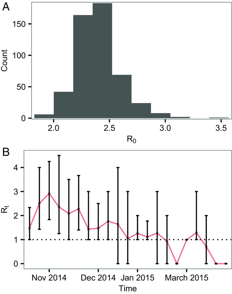
We estimated that has median value 2.39, with 95% credible interval (C.I.) of [2.05, 2.84] (Fig. 1A). We also estimated the time-varying reproductive number (Fig. 1B). The incubation period was estimated to be 6.74 d [1.29, 16.21]. These estimates are broadly consistent with what have been reported (3, 12).
Fig. 1.
Estimates of reproductive number. (A) Posterior distribution of the basic reproductive number, . (B) Posterior distribution of the weekly effective reproductive number, . Bars represent 95% C.I., and red line connects the medians.
The mean of infectious period (i.e., duration from symptoms onset to death/burial) was estimated to be 3.9 d [3.75, 4.0]. Because the transmission tree and times of infection were imputed (Materials and Methods), we were also able to infer the mean generation time of EBOV, which was estimated to be 10.9 d [9.25, 13.01]. Both estimates were lower than that estimated from cases detected within the clinical care system [e.g., mean infectious period 8 d estimated for patients who received clinical care (13) and mean generation time 15.3 d estimated by the WHO (1)]. These discrepancies potentially highlight systematic differences between community-based cases and cases notified in clinical care systems, with terminal community-based cases progressing significantly more rapidly.
Superspreading in Space and Time.
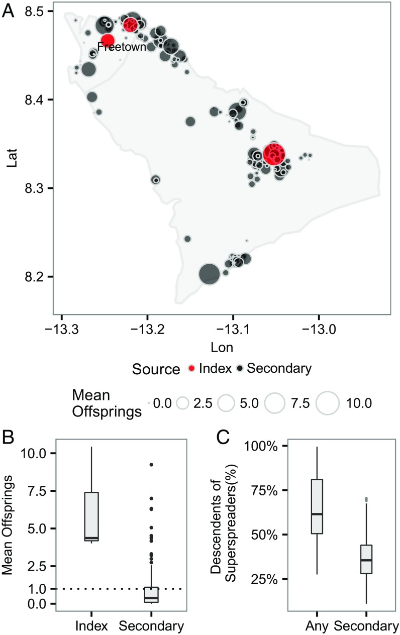
Fig. 2 A and B show a clear asymmetry in the average number of “offspring” at the individual level, quantifying the impact of superspreading. In particular, it was observed that most secondary cases generated less than one offspring on average. Thus, the epidemic growth appeared to be fueled mostly by only a few superspreaders (i.e., the outliers in the boxplot). A common empirical measure of degree-of-transmission heterogeneity and superspreading is the dispersion parameter , assuming that the offspring distribution is a negative binomial with variance , where is the mean (9). Generally speaking, a lower represents a higher degree of transmission heterogeneity and superspreading; and < 1 implies substantial superspreading (compared with a geometric distribution, for which k = 1). Our empirical estimate of k of our inferred mean offspring distribution (including index and secondary) was 0.37, and it is higher (i.e., implies less heterogeneity) than an estimate from an observational study in which was estimated to be 0.16 (10, 11). This discrepancy in the estimate of suggests that our estimate of the degree of superspreading may be conservative (Sensitivity Analysis), although it should be noted their estimate was made based on a study in a different geographical region and time frame. By sampling probabilistically consistent transmission networks among infected individuals (Materials and Methods), we were able to identify whether a case was a descendent of superspreaders by performing a backward search of sampled transmission tree from the casefor each case, we first identified its (most recent) direct infector () from the sampled tree, from where we could subsequently identify the infector of ; We continued this backward searching until we reached an index case [i.e., the root of a (sub)tree]; a superspreader is an ancestor of this case if it happens to be one of the infectors during the backward searching. Fig. 2C shows that a few superspreaders (3% of all of the cases) were responsible, either directly or indirectly, for a substantial proportion (with median 61%) of all of the cases generated, highlighting the key role of these superspreaders in driving the epidemic growthhad the superspreaders been identified and quarantined promptly, a majority of the infections could have been prevented.
Fig. 2.
(A) Spatial distribution of mean number of offspring resulting from initial cases at the individual level. An infection is classified as an index case if it has a posterior probability of importation (i.e., not infected by any cases in the data) >0.5; otherwise, it is classified as a secondary case. Lat, latitude; Lon, longitude. (B) Distribution of mean number of offspring by different sources of infection. (C) Proportion of infected individuals who are direct and indirect descendants of the first five superspreaders (i.e., first five individuals with highest number of mean offspring; note that the choice of five is arbitrary here). “Any” includes superspreaders who were also the index cases (i.e., the roots of transmission trees).
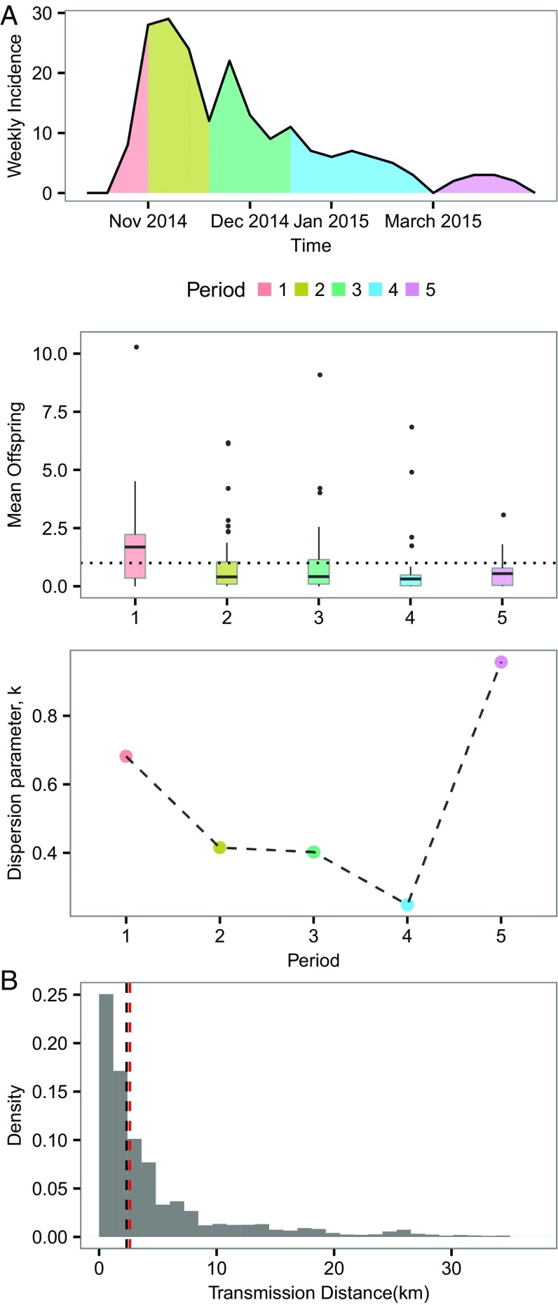
In Fig. 3A, we show the time dependence of superspreading, illustrating that superspreading becomes relatively more important over time (i.e., within 100 d after the epidemic peak). This figure suggests that, after the initial period of fast growth of the epidemic (i.e., time before peak), superspreaders may be crucial to sustaining and fueling epidemic growth and also prolonging the epidemic duration. Near the end of the epidemic (period 5 in Fig. 3A), most cases did not spread, and superspreading was nonsignificant, as reflected by k > 1. Fig. 3B shows that most of the transmission (including superspreading) occurred over relatively short distances (median 2.51 km), indicating that transmission tends to take place at the local community level.
Fig. 3.
Spatial and temporal dependence of superspreading. (A) Reported weekly deaths and inferred mean offspring distributions and the corresponding empirical estimates of at different time periods. The whole time period is divided into five periodsthat is, period 1, from the time of first observation to the time of epidemic peak ; period 2, (, ); period 3, (, ); period 4, (, ); and period 5, from to the time of last observation. Such a dividing was used so that we could use the peak time as a reference point and ensure a similar number of cases in most intervals. (B) Distribution of distance of transmission for all infector–infected pairs. Black dotted line represents the median (2.51 km) of the distribution. Red dotted line represents the median (2.61 km) of the subdistribution in which the infectors are superspreaders (defined as those who has mean offspring more than five here).
Heterogeneity of Infectiousness by Age.
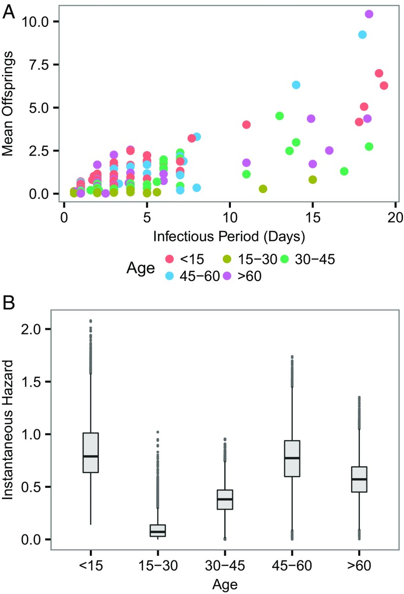
Although superspreading in EBOV was evident and may be partly attributed to unsafe burial practice during the early stage of the outbreak (14), other drivers (e.g., social contact pattern) of this process remain unclear. In Fig. 4A, as expected, the infectious period had a clear positive relationship with mean offspring number. Despite the clear relationship between infectious period and the magnitude of superspreading, this covariate cannot be used as a predictor of superspreading, because it is not known a priori. More importantly, there is a significant difference in instantaneous infectious hazard exerted by different age groups (Fig. 4B)cases <15 and >45 appear to have higher instantaneous transmissibility. Our results suggest that the combination of certain age groups (who have high instantaneous hazard) with a long infectious period (at the right tail of the infectious period distribution) constitutes a key driver of superspreading. The discrepancy of transmissibility in age may be rooted in social contact structure (15) or virological linkages (e.g., potential systematic variation among infected individuals) that cannot be established solely by using epidemiological data (16).
Fig. 4.
Heterogeneity of infectiousness in age. (A) Relation between mean offspring and infectious period. It is worth noting that here an infectious period is strictly referred to the mean of the posterior samples of imputed infectious period of an individual, rather than the assumed universal infectious period distribution. (B) Instantaneous risk exerted by different age groups.
Sensitivity Analysis.
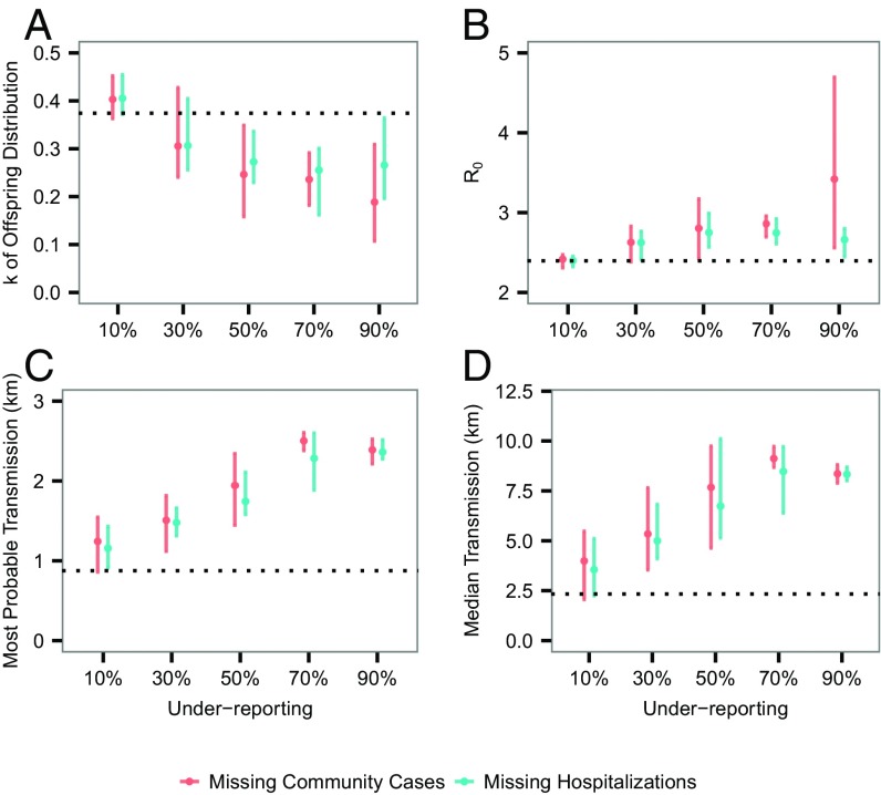
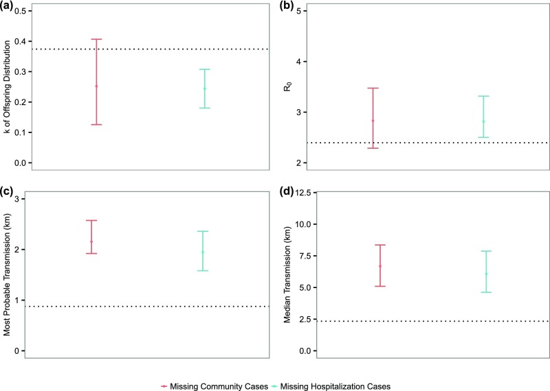
Underreporting is a ubiquitous feature of epidemiological data (17, 18). In this section, we explore the effect of underreporting on our analysis under two probable scenarios: (i) All unreported cases were circulating in the community and not hospitalized; and (ii) all unreported cases were hospitalized and therefore not reported in our database. In both scenarios, we tested with constant underreporting rates, across the whole study period and region, ranging from a very low (10%) to a very high one (90%). Doing so allowed us to investigate the probable lower and upper bound of our estimates. We also tested with time-varying underreporting rates in both scenarios. Details of how to include underreported cases are provided in Materials and Methods.
We focused on investigating the effect on , and transmission distance. Fig. 5A shows that, in general, superspreading should have been even more prominent in the presence of underreporting, compared with our estimate. Such a discrepancy suggests that our estimated degree of superspreading is potentially (at most moderately) conservativefor example, at a constant underreporting rate of 90%, the median of is 0.27 in scenario 2, moderately lower than 0.37 estimated from the baseline analysis. Underreporting appears to have limited effect on the estimated , at least up to underreporting rate of 80% (Fig. 5B). Fig. 5 C and D suggest that, although we can be relatively confident about the most probable transmission distance, it is almost certain that we missed some long-distance transmission events. Assuming a time-varying underreporting rate gives rise to similar results (Fig. S1).
Fig. 5.
Effect of constant underreporting rates on estimates of transmission dynamics. (A) Estimates of . Bars represent the 95% C.I., and dots represent the median values. (B) Estimates of . (C) Estimates of most probable distance of transmission. (D) Estimates of median transmission distance. Dotted lines represent the corresponding estimates using our data. At each underreporting rate, 10 independent simulations and corresponding inference were performed (Materials and Methods).
Fig. S1.
Effect of time-varying underreporting on estimates of transmission dynamics. (A) Estimates of . Bars represent the 95% C.I., and dots represent the median values. (B) Estimates of . (C) Estimates of most probable distance of transmission. (D) Estimates of median transmission distance. Dotted lines represent the corresponding estimates using our data. The underreporting rate is assumed to decrease with a step size 10%, from 90 to 10%, in the course of the epidemic: The study period is divided into nine equal intervals, and each interval takes an underreporting rate that is 10% lower than the previous one.
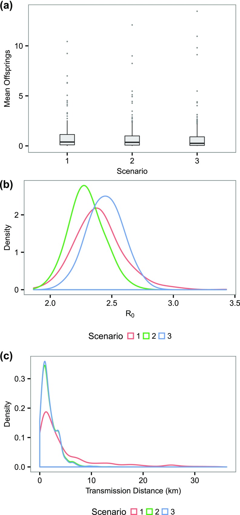
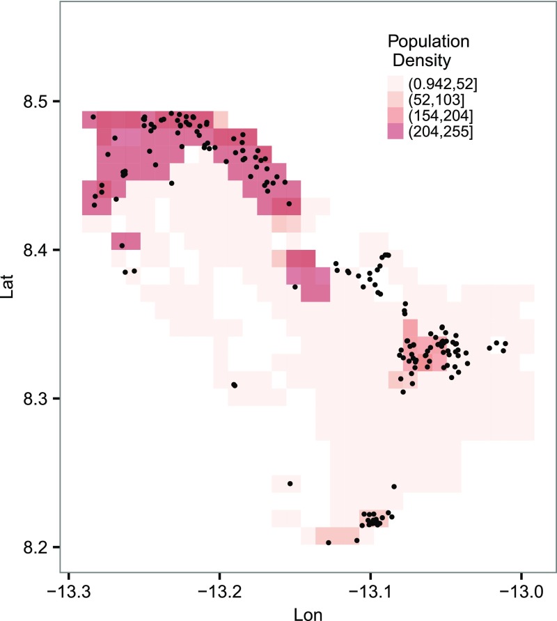
Our model assumed an isotropic spatial dispersal (Materials and Methods). Spatial infectivity, however, may depend on the population densityin particular, it may exhibit a gravity-model pattern that is observed in a few disease systems, including Ebola (19–21). Such gravity models scale the distance-dependent infectious challenge acting on the recipients, by incorporating a “local susceptibility” as a function of the population size of the receiving areathat is, a more populated place is prone to a greater movement influx (of cases) and hence a greater effective infectious challenge. Based on the underlying principles of gravity models, we also investigated the effect of population density on these estimates (Fig. S2), using two different formulations in specifying the local susceptibility. First, without taking into account the population density, we may have missed identifying a few prominent superspreaders at the right tail of the offspring distribution and, hence, underestimated superspreading (Fig. S2A). Conversely, it was shown that population density has no significant effect on (Fig. S2B). Finally, assuming an isotropic dispersal may have slightly biased toward the longer transmission distance (Fig. S2C). Nevertheless, the effects were nonsignificant, mainly due to relatively homogeneous population density where the cases resided (Fig. S3). The parameterization of the incubation period and infectious period were also tested, showing very similar estimates as the baseline case (Tables S1 and S2). We also tested alternative parameterization of priors in Table S3, giving virtually identical results compared with those obtained in the baseline case (see also Materials and Methods).
Fig. S2.
Testing the assumption of an isotropic spatial dispersal. (A) The distribution of mean offsprings under different scenarios. (B) The distribution of R0 under different scenarios. (C) The distribution of transmission distance under different scenarios. Here we considered three scenarios. In scenario 1 (base scenario), we assumed an isotropic dispersal and did not take into account the potential effect of population density. We considered in scenarios 2 and 3 that the dispersal kernel value was “moderated” by the relative population density of the grid that a case resides in. Scenarios 2 and 3 differ in how the population density was normalized (to between ) to obtain the discounting factor: In scenario 2, we normalized according to (1 + population density), and in scenario 3, we normalized according to the absolute scale of population density.
Fig. S3.
Population density and spatial distribution of the cases in the study area. Other than the smaller clusters near the center of the study area, most cases were found in more populated regions. It was noted that the raw grid resolution is (which is too fine to display), and here it is binned into grids for better visualization. Lat, latitude; Lon, longitude.
Table S1.
Testing alternative parameterizations of the incubation period
| Parameterization | Generation time, d | Dispersion parameter, | |
| (baseline) | 10.9 | 2.39 | 0.37 |
| 10.9 | 2.46 | 0.35 | |
| 9.7 | 2.20 | 0.45 |
The mean of generation time, R0, and the dispersion parameter k that quantifies superspreading are shown.
Table S2.
Testing alternative parameterizations of the infectious period
| Parameterization | Generation time, d | Dispersion parameter, | |
| (baseline) | 10.9 | 2.39 | 0.37 |
| 10.3 | 2.39 | 0.40 | |
| 10.43 | 2.40 | 0.38 |
The mean of generation time, R0, and the dispersion parameter k that quantifies superspreading are shown.
Table S3.
Testing alternative uninformative priors
| Priors | Generation time, d | Dispersion parameter, | |
| (baseline) | 10.9 | 2.39 | 0.37 |
| 10.8 | 2.39 | 0.36 |
The mean of generation time, R0, and the dispersion parameter k that quantifies superspreading are shown.
Discussion
Superspreading is a core process for the transmission of many infections (7, 8). However, the importance of superspreading in driving epidemics varies with context. For instance, its impact depends on how it persists over the course of an epidemic. Quantifying superspreading and identifying scenarios where it is more likely to occur can facilitate refining future epidemics predictions and help in devising targeted intervention strategies that may outperform population-level control measures (9). To date, a systematic understanding of how EBOV has been (super)spreading in the recent outbreak in Western Africa is lacking, particularly in terms of individual-level covariates, and across the spatiotemporal setting. The key contributions of this work are to highlight and quantify the importance of superspreading and to show that it is in some senses systematic.
Community-based surveillance data offer a valuable opportunity to study superspreading, by focusing on nonhospitalized cases that may have been involved in superspreading events and not detected by formal surveillance. Here, we introduce a continuous-time spatiotemporal model that integrates individual spatial information with other epidemiological information of community-based cases and deploy it to quantify superspreading and its drivers for EBOV. Our framework enabled us to sample likely realizations of the unobserved transmission network among cases from which the offspring distribution of each case could be inferred, providing explicitly a machinery for understanding superspreading in space and time.
Our analysis is broadly consistent with previous work, indicating values of of 2.39 [2.05, 2.84] for the outbreak in Sierra Leone (in particular, close to the 2.53 estimated in ref. 22). Our results show that EBOV exhibited a prominent superspreading pattern shared by SARS and MERS (7, 8, 23) [e.g., was estimated to be 0.16 for SARS (9)], which reinforces the finding that superspreading occurred during the recent EBOV outbreak (10).
We also extended previous analyses by showing that a substantial proportion of secondary cases were either direct or indirect descendants of a small number of superspreaders, underscoring the importance of superspreading in driving the epidemicthat is, had the superspreaders been identified and quarantined promptly, 61% of the infections could have been prevented. Furthermore, we show that superspreaders may have particular importance in driving and sustaining the epidemic progression over the course of the outbreak. The increasing relative importance of superspreading over the later stages of the outbreak (Fig. 3A) is consistent with the rising availability of hospital beds (5)that is, later in the outbreak, most infected individuals were able to get a bed at an Ebola treatment center (ETC) and largely did not further transmit; as a result, those superspreaders in the community who did not make it to ETCs may have played an increasingly important role in sustaining the epidemic by generating more secondary cases. Our results also suggest that Ebola transmission may have disproportionately affected the local community, because we estimate a relatively short transmission distance. This estimated distance has implications for implementation of regional control measures. Identifying individuals who have the profile (socially or culturally) of being at greater risk of causing superspreading events is crucial for implementing targeted interventions.
We reveal that age-dependent social contact structure may play an important role in (super)spreading EBOV in the local community. Specifically, our results identify age groups that have higher instantaneous transmissibility and show that cases in the more infectious age groups tend to be superspreaders when combined with a relatively long infectious duration. One plausible explanation, from the social perspective, may be that the young and old are much more likely to have (and infect) lots of visitors, compared to other age groups; a parallel corollary is that the young and old might be more likely to have others caring for them. Also, our results highlight systematic differences between community-based cases and cases notified in clinical care systems, with terminal community-based cases progressing significantly more rapidly. Our results stress the importance of characterizing superspreading of EBOV, enhance current understandings of its spatiotemporal dynamics, and highlight the potential importance of targeted control measuresfor example, during the 2014–2015 EBOV epidemic, millions of dollars were spent implementing message strategies about Ebola prevention and control across entire countries; our results suggest that message strategies targeting individuals with higher risk may be useful to prevent superspreading events and the persistence of the outbreak.
There are limitations of our results. First of all, although community-based surveillance data complement formal surveillance by detecting cases that did not interface with clinical care, they contain only partial information about the epidemic, with hospitalized cases omitted. Also, it is possible that, by underreporting some community cases who generated subsequent cases, certain reported cases may be falsely attributed as sources of infection for those subsequent cases, overestimating the degree of superspreading. Accordingly, our sensitivity analysis evaluated the impact of these sources of underreporting, showing that our estimated degree of superspreading may in fact be conservative and represents a lower boundsuperspreading in EBOV may be even more prominent in reality (Fig. 5). It is also worth noting that, by considering only safe burials, which tend to be less transmissible (relative to those did not receive safe burials) among deaths (14), our estimate of superspreading may have been conservative. Conversely, because it was reported that individuals who eventually died might have a higher intrinsic transmissibility (24), our analysis might bias toward high transmitters by only using death data. Our methodology represents a transmission network-based approach that focused on constructing transmission trees among cases (25–28). Although such an approach captures contacts that caused infections, it does not account for “unsuccessful” contacts that correspond to escaped infections. Future theoretical work will need to include such contacts. Nevertheless, because unsuccessful contacts are not parts of the transmission chain, ignoring them has limited effect on the transmission tree or on many overall topological characteristics (e.g., average number of offspring of an infected case) (25, 28, 29). Finally, although our analysis reveals the importance of age as demographic determinants of superspreading, future work in linking them with virological factors (e.g., age-specific viral loads) may shed further light (16).
Materials and Methods
Spatiotemporal Transmission Model.
We developed a continuous-time spatiotemporal transmission model that allowed us to sample the transmission tree among cases, integrating observed spatial and temporal individual data. This approach allowed us to infer explicitly the mean offspring distribution of each case. Specifically, the total probability of individual becoming infected during time period was given by
| [1] |
where is the set of all infectious individuals at time , is the background rate of infection, and is the age-specific instantaneous infection hazard of a case in . We allowed five-level according to the age—that is, we had for age between , for age between , for age between , for age between , and for age >60. , also known as a dispersal kernel, characterized the dependence of the infectious challenge from infectious to as a function of distance between them. Here, we have . After the infection, it was assumed that individual would go through an incubation period (i.e., time from infection to symptoms onset) and an infectious period (i.e., time from onset to death). The incubation period was assumed to follow a gamma distribution distribution (where and are mean and SD, respectively), and the infectious period followed an exponential distribution with mean . We assumed the infectiousness started from the symptoms onset time. It was noted that unknown contacts corresponding to escaped infections were not taken into account in our framework, resulting in a likelihood function that accounted for only successful infectious contacts (SI Text)that is, our approach essentially represented a transmission network-based inference, where the focus was to construct the transmission tree among infected individuals (25–28).
Data Augmentation and Model Fit and Validation.
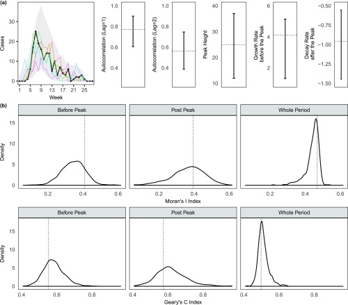
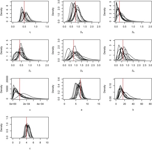
We estimated (i.e., the parameter vector) in the Bayesian framework by sampling it from the posterior distribution , where is the observed data. Denoting the likelihood by , the posterior distribution of is , where is prior distribution for . Weak uniform priors for parameters in were used (Table S4). Markov chain Monte Carlo (MCMC) techniques (30) were used to obtain the posterior distribution. The unobserved infection times and transmission network were imputed in the MCMC. Sampled transmission networks were recorded and used to infer the offspring distribution of each case. Details of the likelihood function and the MCMC algorithm are given in SI Text. Model fit was assessed by comparing the observed data with those simulated from the estimated model, suggesting a good fit (Fig. S4). Furthermore, for validating the implementation of our inference procedures, we generated multiple sets of pseudodata from the modal process and demonstrated that we could successfully reestimate the model parameters (Fig. S5).
Table S4.
Prior and posterior distributions of model parameters
| Parameter | Median [95% C.I.] | Prior |
| , infectivity of first age group | 0.76 [0.42, 1.39] | U(0,100) |
| , infectivity of second age group | 0.07 [0.002, 0.36] | U(0,100) |
| , infectivity of third age group | 0.4 [0.1, 0.66] | U(0,100) |
| , infectivity of fourth age group | 0.79 [0.27, 1.25] | U(0,100) |
| , infectivity of fifth age group | 0.56 [0.23, 0.92] | U(0,100) |
| , spatial kernel parameter | 0.42 [0.06, 0.87] | U(0,100) |
| (), background hazard | 4.6 [0.21, 12] | U(0,100) |
| , mean of the incubation period | 6.87 [5.34, 8.50] | U(0,100) |
| , SD of the incubation period | 4.02 [2.44, 5.44] | U(0,100) |
| , mean (and SD) of the infectious period | 3.96 [3.41, 4.60] | U(0,100) |
Fig. S4.
Assessing the model fit. We used the estimated model to simulate (500 times) forward the transmission path and timings of events (i.e., infection time, onset time, and death time). (A) Comparison of the observed weekly temporal distribution of the cases with that summarized from the simulated data. Gray area represents the 95% C.I., and the black dots and line are the observed data, with 5 of 500 random realizations (colored lines) of the simulated epidemics imposed. We compared the temporal autocorrelations (at lag = 1 and lag = 2) of the observed and simulated epidemics. We also compared the peak height, the growth rate before peak, and decay rate after peak between the observed and simulated (the growth and decay rates correspond to the slopes of best-fitted linear lines to the observed or simulated data). Dotted lines represent the values of the summary statistics corresponding to the observed data. (B) Comparison of the observed spatial autocorrelation and the simulated. Here we used two common measures, Moran’s I and Geary’s C indices (33, 34), which range from −1 to 1 (a value close 1 indicates strong clustering and close to −1 indicates strong dispersion). Dotted lines represent the values of the summary statistics corresponding to the observed data.
Fig. S5.
Checking of the implementation of the inference procedures. We simulated 10 independent pseudodata from the model, with the model parameter values close to the posterior means obtained from fitting with the real dataset. The model is then fitted to each of the simulated datasets, and the resultant posterior distributions of the model parameters are shown. The true values of the model parameters are indicated by the red lines.
Testing Underreporting.
We divided the observational period into many 3-d-wide intervals. Within each time interval, we had the total number of unreported cases , where and were the observed cases in the interval and the assumed underreporting rate, respectively. Burial times and symptoms-onset time of these unreported cases were drawn from the empirical distribution of the observed cases. Finally, these cases were distributed spatially by using the empirical distribution of (normalized) population densities across the study area. We also tested an underreporting rate that decreases with time (Fig. S1). For the scenario that considers unreported hospitalized cases, we drew the time from symptoms onset to hospitalization from the truncated above (at 7 d) empirical infectious period distribution of observed cases, effectively resulting in a shorter infectious period for unreported cases. These artificially generated data were combined with the observed data and fitted with our model.
SI Text
Likelihood Function.
Let be the vector of the exposure/infection times of the cases, the times of becoming infectious, and the death times. The epidemic was observed up to time . The incubation period was assumed to be a two-parameter density function characterized by parameters and ; similarly, for the infectious period (i.e., time from start of infectiousness to death), with density function . Finally, let be the source of infection of case and be the collection set for cases. The likelihood of the parameter vector given complete data can be expressed as
| [S1] |
where
| [S2] |
is the (unnormalized) probability of case to be an index case of infected by case , respectively, and
| [S3] |
is the probability of case to have not been infected up to time , where is the set of all infectious individuals at time .
MCMC Algorithm.
Parameters in were updated sequentially with a standard random-walk Metropolis–Hastings (M-H) algorithm (30, 31). For example, a new parameter value was proposed from a normal distribution centered on the current value of , that is,
| [S4] |
where controls the step size of the random-walk. Elements in infection times vector were also treated as unobserved model parameters and were imputed in the same manner (30). Approximately 10% of the cases had invalid records of symptom onset time; hence, corresponding elements in were also imputed similarly. We used (weak) uniform priors with upper bounds for all model parameters, and the maximum of the incubation period was assumed to be 21 d (32). Details of the priors and obtained posteriors are shown in Table S4.
Denote as the set of eligible candidates for a new source of infection for (i.e., contains a set of cases whose are infectious at ). We propose a new infecting source to be with probability
| [S5] |
Note that the background infection can be accommodated by adding a permanent infectious source presenting an additional challenge of strength to individual . A newly proposed source is accepted or rejected depending on the M-H acceptance probability (29).
Acknowledgments
This work was supported by Bill & Melinda Gates Foundation Grant OPP1091919; the RAPIDD program of the Science and Technology Directorate Department of Homeland Security and the Fogarty International Center, National Institutes of Health; and the UK Medical Research Council (MRC). S.F. was also supported by MRC Career Award in Biostatistics MR/K021680/1.
Footnotes
The authors declare no conflict of interest.
This article is a PNAS Direct Submission.
This article contains supporting information online at www.pnas.org/lookup/suppl/doi:10.1073/pnas.1614595114/-/DCSupplemental.
References
- 1.Team WER, et al. Ebola virus disease in West Africa—the first 9 months of the epidemic and forward projections. N Engl J Med. 2014;371(16):1481–1495. doi: 10.1056/NEJMoa1411100. [DOI] [PMC free article] [PubMed] [Google Scholar]
- 2.Team WER, et al. West African Ebola epidemic after one year slowing but not yet under control. N Engl J Med. 2015;372(6):584–587. doi: 10.1056/NEJMc1414992. [DOI] [PMC free article] [PubMed] [Google Scholar]
- 3.Chretien JP, Riley S, George DB. Mathematical modeling of the West Africa Ebola epidemic. eLife. 2015;4:e09186. doi: 10.7554/eLife.09186. [DOI] [PMC free article] [PubMed] [Google Scholar]
- 4.Fisman D, Khoo E, Tuite A. Early epidemic dynamics of the West African 2014 Ebola outbreak: Estimates derived with a simple two-parameter model. PLoS Curr Outbreaks. 2014 doi: 10.1371/currents.outbreaks.89c0d3783f36958d96ebbae97348d571. [DOI] [PMC free article] [PubMed] [Google Scholar]
- 5.Camacho A, et al. Temporal changes in Ebola transmission in Sierra Leone and implications for control requirements: A real-time modelling study. PLoS Curr Outbreaks. 2015 doi: 10.1371/currents.outbreaks.406ae55e83ec0b5193e30856b9235ed2. [DOI] [PMC free article] [PubMed] [Google Scholar]
- 6.Weitz JS, Dushoff J. Modeling post-death transmission of Ebola: Challenges for inference and opportunities for control. Sci Rep. 2015;5:8751. doi: 10.1038/srep08751. [DOI] [PMC free article] [PubMed] [Google Scholar]
- 7.Galvani AP, May RM. Epidemiology: Dimensions of superspreading. Nature. 2005;438(7066):293–295. doi: 10.1038/438293a. [DOI] [PMC free article] [PubMed] [Google Scholar]
- 8.Kucharski A, Althaus C. The role of superspreading in Middle East respiratory syndrome coronavirus (MERS-CoV) transmission. Euro Surveill. 2015;20(25):14–18. doi: 10.2807/1560-7917.es2015.20.25.21167. [DOI] [PubMed] [Google Scholar]
- 9.Lloyd-Smith JO, Schreiber SJ, Kopp PE, Getz W. Superspreading and the effect of individual variation on disease emergence. Nature. 2005;438(7066):355–359. doi: 10.1038/nature04153. [DOI] [PMC free article] [PubMed] [Google Scholar]
- 10.Althaus CL. Ebola superspreading. Lancet Infect Dis. 2015;15(5):507–508. doi: 10.1016/S1473-3099(15)70135-0. [DOI] [PMC free article] [PubMed] [Google Scholar]
- 11.Faye O, et al. Chains of transmission and control of Ebola virus disease in Conakry, Guinea, in 2014: An observational study. Lancet Infect Dis. 2015;15(3):320–326. doi: 10.1016/S1473-3099(14)71075-8. [DOI] [PMC free article] [PubMed] [Google Scholar]
- 12.Stadler T, Kühnert D, Rasmussen DA, du Plessis L. Insights into the early epidemic spread of Ebola in Sierra Leone provided by viral sequence data. PLoS Curr Outbreaks. 2014 doi: 10.1371/currents.outbreaks.02bc6d927ecee7bbd33532ec8ba6a25f. [DOI] [PMC free article] [PubMed] [Google Scholar]
- 13.Bah EI, et al. Clinical presentation of patients with Ebola virus disease in Conakry, Guinea. N Engl J Med. 2015;372(1):40–47. doi: 10.1056/NEJMoa1411249. [DOI] [PubMed] [Google Scholar]
- 14.Nielsen CF, et al. Improving burial practices and cemetery management during an Ebola virus disease epidemic—Sierra Leone, 2014. MMWR Morb Mortal Wkly Rep. 2015;64(1):20–27. [PMC free article] [PubMed] [Google Scholar]
- 15.Anderson R, May R. Age-related changes in the rate of disease transmission: Implications for the design of vaccination programmes. J Hyg (Lond) 1985;94(3):365–436. doi: 10.1017/s002217240006160x. [DOI] [PMC free article] [PubMed] [Google Scholar]
- 16.Geoghegan JL, Senior AM, Di Giallonardo F, Holmes EC. Virological factors that increase the transmissibility of emerging human viruses. Proc Natl Acad Sci USA. 2016;113(15):4170–4175. doi: 10.1073/pnas.1521582113. [DOI] [PMC free article] [PubMed] [Google Scholar]
- 17.Doyle TJ, Glynn MK, Groseclose SL. Completeness of notifiable infectious disease reporting in the United States: An analytical literature review. Am J Epidemiol. 2002;155(9):866–874. doi: 10.1093/aje/155.9.866. [DOI] [PubMed] [Google Scholar]
- 18.Brabazon E, O’farrell A, Murray C, Carton M, Finnegan P. Under-reporting of notifiable infectious disease hospitalizations in a health board region in Ireland: Room for improvement? Epidemiol Infect. 2008;136(2):241–247. doi: 10.1017/S0950268807008230. [DOI] [PMC free article] [PubMed] [Google Scholar]
- 19.Viboud C, et al. Synchrony, waves, and spatial hierarchies in the spread of influenza. Science. 2006;312(5772):447–451. doi: 10.1126/science.1125237. [DOI] [PubMed] [Google Scholar]
- 20.Yang W, et al. Transmission network of the 2014–2015 Ebola epidemic in Sierra Leone. J R Soc Interface. 2015;12(112):20150536. doi: 10.1098/rsif.2015.0536. [DOI] [PMC free article] [PubMed] [Google Scholar]
- 21.Xia Y, Bjørnstad ON, Grenfell BT. Measles metapopulation dynamics: A gravity model for epidemiological coupling and dynamics. Am Nat. 2004;164(2):267–281. doi: 10.1086/422341. [DOI] [PubMed] [Google Scholar]
- 22.Althaus CL. Estimating the reproduction number of Ebola virus (EBOV) during the 2014 outbreak in West Africa. PLoS Curr Outbreaks. 2014 doi: 10.1371/currents.outbreaks.91afb5e0f279e7f29e7056095255b288. [DOI] [PMC free article] [PubMed] [Google Scholar]
- 23.Cowling BJ, et al. Preliminary epidemiologic assessment of MERS-CoV outbreak in South Korea, May to June 2015. Euro Surveill. 2015;20(25):7–13. doi: 10.2807/1560-7917.es2015.20.25.21163. [DOI] [PMC free article] [PubMed] [Google Scholar]
- 24.Yamin D, et al. Effect of Ebola progression on transmission and control in Liberia. Ann Intern Med. 2015;162(1):11–17. doi: 10.7326/M14-2255. [DOI] [PMC free article] [PubMed] [Google Scholar]
- 25.Haydon DT, et al. The construction and analysis of epidemic trees with reference to the 2001 UK foot-and-mouth outbreak. Proc Biol Sci. 2003;270(1511):121–127. doi: 10.1098/rspb.2002.2191. [DOI] [PMC free article] [PubMed] [Google Scholar]
- 26.Cottam EM, et al. Integrating genetic and epidemiological data to determine transmission pathways of foot-and-mouth disease virus. Proc Biol Sci. 2008;275(1637):887–895. doi: 10.1098/rspb.2007.1442. [DOI] [PMC free article] [PubMed] [Google Scholar]
- 27.Leventhal GE, et al. Inferring epidemic contact structure from phylogenetic trees. PLoS Comput Biol. 2012;8(3):e1002413. doi: 10.1371/journal.pcbi.1002413. [DOI] [PMC free article] [PubMed] [Google Scholar]
- 28.Morelli MJ, et al. A Bayesian inference framework to reconstruct transmission trees using epidemiological and genetic data. PLoS Comput Biol. 2012;8:e1002768. doi: 10.1371/journal.pcbi.1002768. [DOI] [PMC free article] [PubMed] [Google Scholar]
- 29.Lau MS, Marion G, Streftaris G, Gibson G. A systematic Bayesian integration of epidemiological and genetic data. PLoS Comput Biol. 2015;11(11):e1004633. doi: 10.1371/journal.pcbi.1004633. [DOI] [PMC free article] [PubMed] [Google Scholar]
- 30.Gibson GJ, Renshaw E. Estimating parameters in stochastic compartmental models using Markov chain methods. Math Med Biol. 1998;15(1):19–40. [Google Scholar]
- 31.Chib S, Greenberg E. Understanding the Metropolis-Hastings algorithm. Am Stat. 1995;49(4):327–335. [Google Scholar]
- 32.Briand S, et al. The international Ebola emergency. N Engl J Med. 2014;371(13):1180–1183. doi: 10.1056/NEJMp1409858. [DOI] [PubMed] [Google Scholar]
- 33.Getis A. Spatial interaction and spatial autocorrelation: A cross-product approach. Environ Plan A. 1991;23(9):1269–1277. [Google Scholar]
- 34.Lau MSY, Marion G, Streftaris G, Gibson GJ. New model diagnostics for spatio-temporal systems in epidemiology and ecology. J R Soc Interface. 2014;11:20131093. doi: 10.1098/rsif.2013.1093. [DOI] [PMC free article] [PubMed] [Google Scholar]


