Satellite-based assessment of yield variation and its determinants in smallholder African systems

Significance

Improvements in agricultural productivity in developing countries are thought to play a key role in poverty reduction. Unfortunately, such productivity remains poorly measured throughout much of the world, hampering efforts to evaluate and target productivity-enhancing interventions. Using high-resolution satellite imagery in combination with field data we collected from thousands of smallholder plots in Kenya, we show that satellite imagery can be used to estimate and understand yield variation at the field scale across African smallholders. Our results suggest a range of potential capabilities, including the inexpensive measurement of the impact of specific interventions, the broader characterization of the source and magnitude of yield gaps, and the development of financial products aimed at African smallholders.

Abstract

The emergence of satellite sensors that can routinely observe millions of individual smallholder farms raises possibilities for monitoring and understanding agricultural productivity in many regions of the world. Here we demonstrate the potential to track smallholder maize yield variation in western Kenya, using a combination of 1-m Terra Bella imagery and intensive field sampling on thousands of fields over 2 y. We find that agreement between satellite-based and traditional field survey-based yield estimates depends significantly on the quality of the field-based measures, with agreement highest (${\text{R}}^2$ up to 0.4) when using precise field measures of plot area and when using larger fields for which rounding errors are smaller. We further show that satellite-based measures are able to detect positive yield responses to fertilizer and hybrid seed inputs and that the inferred responses are statistically indistinguishable from estimates based on survey-based yields. These results suggest that high-resolution satellite imagery can be used to make predictions of smallholder agricultural productivity that are roughly as accurate as the survey-based measures traditionally used in research and policy applications, and they indicate a substantial near-term potential to quickly generate useful datasets on productivity in smallholder systems, even with minimal or no field training data. Such datasets could rapidly accelerate learning about which interventions in smallholder systems have the most positive impact, thus enabling more rapid transformation of rural livelihoods.

Improving the productivity of smallholder farmers is thought to be a key component of the effort to reduce global poverty and increase food security (1). Despite the importance of agriculture in these dual goals, however, the productivity of most smallholders around the world remains poorly measured. Agricultural statistics at the national level in developing countries are often unreliable and tend to be poorest in countries where productivity improvements are most needed (2), and systematic data at the subnational or field scale are unavailable in most of these countries. This absence of data on agriculture is a serious constraint to both research and policy, making it difficult to measure productivity gaps, understand why these gaps exist, and evaluate programs aimed at improving overall productivity.

Various strategies have been proposed to plug these data gaps. One promising approach has been the design and implementation of a new wave of nationally representative household panel surveys that contain detailed agricultural modules (3). These ongoing surveys, orchestrated by the World Bank and currently under implementation across multiple African countries, promise to increase understanding of African agriculture. Another approach has been the implementation of smaller-scale and more targeted data collection efforts, for instance to measure the productivity impact of a farm-level intervention in a randomized control trial (RCT) (4, 5). These RCTs enable causal inferences about which factors most constrain productivity, in contrast to studies that rely on correlations (6). Both types of studies, however, rely on expensive field surveys that remain difficult to scale to large areas and can be plagued by considerable inaccuracies in self-reported data (2).

As an alternate approach, researchers have long recognized the potential for remote sensing to improve understanding of agricultural systems, with multiple decades of research demonstrating how satellite imagery can provide insight on these systems at a variety of scales (7). Understanding the magnitude and sources of productivity differences (“yield gaps”) is typically enhanced by data at the field scale (8), and satellite-based insights at this scale have largely come from developed countries or from intensive commercial systems in certain developing countries. In these settings, relatively large field sizes can easily be resolved in existing imagery, and trustworthy ground data often exist with which to calibrate and evaluate satellite-derived productivity estimates (7, 9).

Gaining similar insight into smallholder systems in developing countries has proved more challenging, due both to a lack of available ground data and to difficulty distinguishing the field sizes typical in smallholder systems using commonly available imagery [e.g., Landsat, a US Geological Survey (USGS) and NASA satellite program that has been collecting 30-m imagery for more than three decades (10)]. For instance, global positioning system (GPS)-based measures of plot area from recent household surveys in four African countries indicate that 25% of fields in these countries are less than 0.5 acre in size and more than half of the fields are smaller than 1 acre (11). With Landsat-resolution imagery, the majority of fields in these countries are therefore covered by just a few pixels at most, which given irregular field boundaries and a highly heterogeneous growing environment limits the ability to derive meaningful productivity estimates. New satellites are beginning to solve the resolution constraint, however, with multiple “cubesat” companies now providing 5-m or finer-resolution data at much lower cost than previously available for much of the world and the European Space Agency’s Sentinel-2 sensor providing 10-m resolution public data since mid-2015 (12).

Here we combine 1-m imagery from one of these commercial providers (TerraBella, formerly Skybox, a Google subsidiary) with field data we collected on thousands of smallholder fields over 2 y in western Kenya, a densely populated and intensively farmed rural region in East Africa where maize is the primary crop. We use these data to generate and evaluate field-scale productivity estimates for maize, testing two approaches to converting images into yield estimates: a calibrated approach based on regressions that relate field-measured yields to satellite-derived vegetation indexes (VIs) and a recently introduced uncalibrated approach that uses output from crop simulation models as training data (13) (Methods). The advantage of the uncalibrated approach is that it does not rely on ground data and is thus easily scaled to new periods and regions.

A main empirical challenge in assessing performance of satellite measures is that “true” productivity is unobserved, as available ground-based measures of yield are based on likely imperfect farmer-reported measures of either production or plot area (or both). Typical approaches to obtaining more “objective” measures of yield by having trained field teams harvest small subplots within individual cultivated plots (so-called “crop cuts”) are useful for generating accurate regional-scale yield estimates, but do not clearly outperform farmer self-reports for estimating productivity at the field scale given the high within-field heterogeneity in productivity that is characteristic of smallholder fields (14, 15).

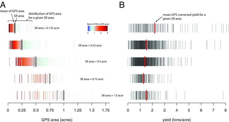
Four issues are particularly challenging in our smallholder context: (i) Farmer self-reported (SR) field area can be a poor measure of true area, with a tendency to round to approximate values and over-report areas for small fields. Fig. 1A compares SR areas with those measured by walking field boundaries with a GPS for fields visited at our study site in 2015, illustrating substantial discrepancies and a tendency to over-report area on average and by as much as a factor of 5 for fields $<$0.5 acre, consistent with other recent studies (11). (ii) SR production is similarly rounded, such as (in our Kenyan setting) to a unit of a 90-kg bag. This leads to errors that are especially problematic for small fields, as suggested by the much higher variance of yield estimates for fields $<$0.5 acre in Fig. 1B. (iii) Geolocation accuracies in both imagery and field data can cause comparisons to be for slightly different areas, which is again an issue that is most problematic on smaller fields. (iv) Maize is often intercropped with a variety of other crops—particularly beans in our context—and the production of these other crops is not often measured. In our study, we simply recorded the presence of other crops but did not ask farmers to estimate production for nonmaize crops.

Fig. 1.

(A) Comparison of self-reported (SR) plot area with GPS-measured area for study fields, 2015 study season. Each row shows the distribution of GPS-measured area for a given SR area, with colors indicating the ratio of SR to GPS area; each vertical line is the estimate for an individual plot. Solid black line reports the mean of SR area and dotted black line the mean of GPS area. All fields in a given row have the same self-reported area. (B) Distribution of estimated yield (SR production/GPS area) by SR area. Both mean and variance of estimated yield are larger on smaller plots.

To disentangle these issues, we examine agreement between satellite-based and farmer-reported yield estimates as a function of field size, for pure maize vs. intercropped fields and for SR vs. GPS-based measures of area. Better agreement on larger, GPS-measured, and/or purestand fields would be consistent with lower error in both field- and satellite-based estimates. We then evaluate the relative performance of different image resolutions, different vegetation indexes, and different calibration approaches—issues that will be important if our approach is to be scaled across regions and years.

Results

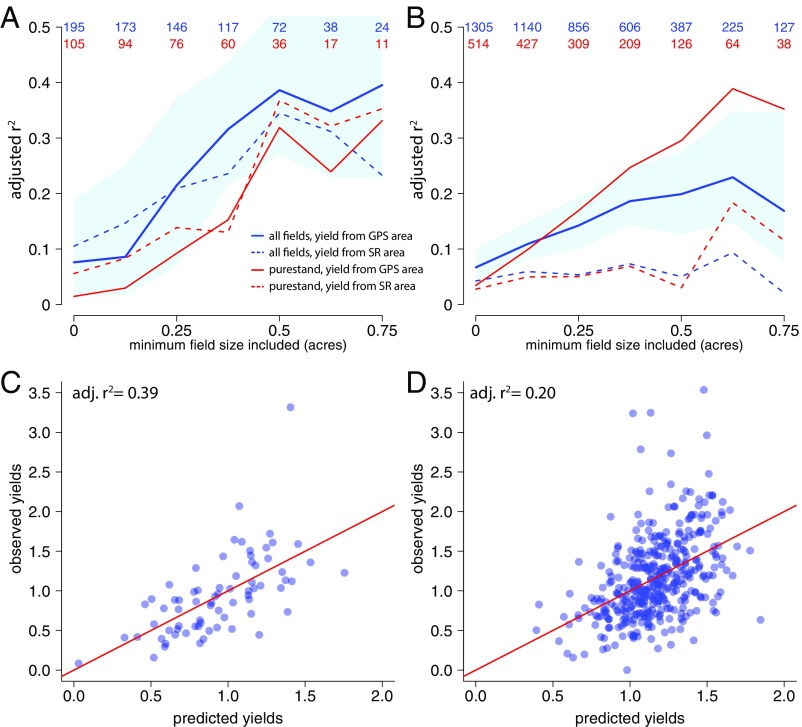
In both the 2014 and 2015 growing seasons, we find that agreement between ground-measured and satellite-derived calibrated maize yield estimates is consistently better on larger fields, as measured by adjusted R² (Fig. 2 A and B). Agreement between the two measures is also higher in most cases (but not always) when using GPS-based area rather than SR area. These results are consistent with the expectation that errors in both the field data and satellite estimates are reduced at larger field sizes, strengthening agreement. Most importantly, we find in both years fairly strong agreement between the satellite-based and field-based yield estimates for fields where confidence in the field data is highest. For fields of at least 0.5 acre, calibrated satellite estimates explain 15–40% of the variation in GPS-corrected farmer self-reported yields (Fig. 2 C and D). Despite having fewer images in 2014, explanatory power is higher in 2014 relative to 2015, which we attribute in part to higher yield variance in the ground data in 2014. Evidence on whether estimates for purestand fields outperform estimates for intercropped fields is unclear, with better performance for purestand fields in 2015 but slightly lower performance in 2014.

Fig. 2.

Performance of VIs in predicting GPS-corrected farmer self-reported yields. (A and B) Performance (adjusted $r^2$) as a function of field size for 2014 (A) and 2015 (B). Colors compare all (blue) vs. purestand field (red), and lines compare GPS-corrected area (solid) and self-reported area (dashed). Blue shaded region reports 95% confidence interval on the all-field, GPS-corrected estimate. Numbers at top of A and B show number of fields included in each estimate. (C) Observed vs. predicted yields on fields $>$0.5 acre, 2014. (D) Same as C for 2015.

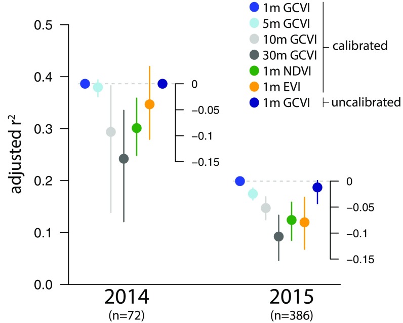
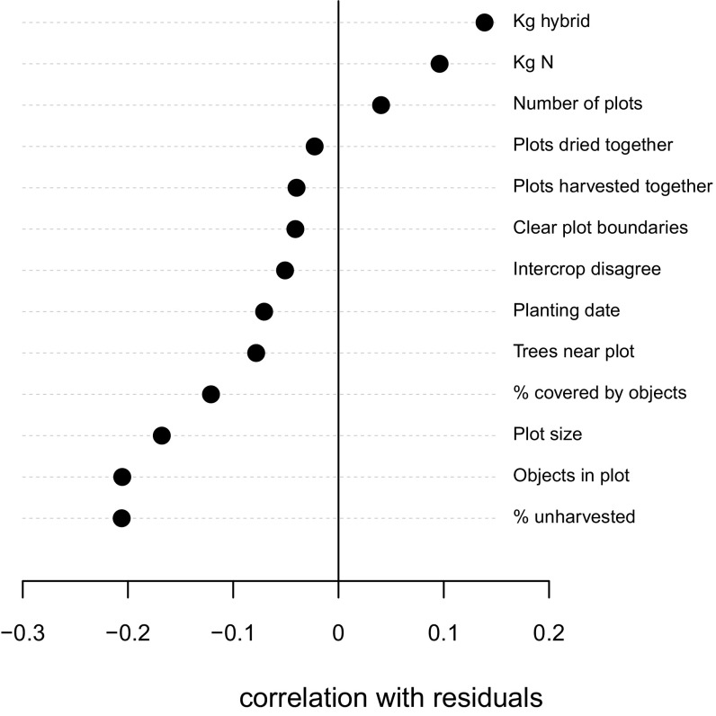
We also find that our preferred measure of canopy greenness (green chlorophyll vegetation index, GCVI) significantly outperforms more traditional vegetation indexes such as the normalized difference vegetation index (NDVI) and enhanced vegetation index (EVI) in both study seasons (Fig. 3). Reflectance at green wavelengths (used in GCVI) is known to be more responsive than red reflectance (used in NDVI and EVI) to variations in leaf chlorophyll concentration (16, 17), and thus it is likely that GCVI captures differences in nutrient deficiency that are correlated with yield. This interpretation is bolstered by the fact that residuals from our model were positively correlated with farmer-reported inputs (Fig. S1), meaning that reflectance indexes were only partly able to capture the effects of nutrient stress on yields, with GCVI more suited to this challenge than NDVI or EVI. Residuals were negatively correlated with other potentially sensible features of the plot, such as the presence of trees near or inside the plot and the percentage of the planted area that was not harvested (with unharvested area typically related to crop waterlogging, theft, or pest or animal intrusion). Other factors such as the presence of weeds likely also reduced the predictive performance of satellite-based estimates, but we did not obtain quantitative measures for these other factors and so could not directly assess their importance.

Fig. 3.

Higher-resolution images outperform coarser images, and GCVI outperforms other vegetation indexes, in predicting GPS-corrected farmer self-reported yields; calibrated estimates outperform uncalibrated ones in 2015 but not in 2014. Solid circles report explanatory power (adjusted $R^2$; left axis) for calibrated 1-m, 5-m, 10-m, and 30-m GCVI and 1-m NDVI and uncalibrated 1-m GCVI, and lines represent 95% confidence interval of difference in adjusted $R^2$ relative to calibrated 1-m GCVI (Inset axes). Sample is fields $>$0.5 acre.

Fig. S1.

Correlation between residuals from yield prediction and other production and/or management factors, for 2015 growing season and fields $>$0.5 acre.

Our results indicate substantial potential of satellite sensors to monitor maize yields in smallholder fields, using traditional calibrated approaches to deriving yield estimates from imagery. Three issues are particularly relevant to the scalability and applicability of this approach. The first one is whether the 1-m resolution of Terra Bella is essential for resolving yields on individual fields or whether coarser resolutions that are potentially available more widely and at lower cost would be as useful. To test this, we aggregated the satellite data to 5-m, 10-m, and 30-m resolution, with 5 m representing sensors such as RapidEye and Planet Scope, 10 m representing Sentinel, and 30 m representing Landsat. Although the performance deteriorates very slightly at 5 m, it still appears useful for crop monitoring (Fig. 3). Explanatory power at 10 m is roughly 75% of what it is at 1 m, and by 30-m resolution explanatory power falls by roughly half compared with 1 m. This indicates substantial benefit to using higher-resolution imagery for yield prediction in smallholder systems, but also suggests that lower-resolution imagery is not without value in the absence of alternatives.

A second issue is whether one can avoid the need for ground calibration by instead using crop model simulations as training data (13). To test this, crop simulations were run for the study years using daily weather data from a local station and then used to estimate a regression model to predict yields from 1-m GCVI (Methods). For the 2014 season in which only one image was available, the explanatory power of calibrated and uncalibrated predictions is identical (as both approaches are univariate regressions with a rescaled independent variable). For the 2015 season, where two images were available, uncalibrated predictions are only modestly less predictive than calibrated predictions.

A third issue is whether imperfect agreement between ground- and satellite-based yield estimates is driven entirely by noise in the satellite measures or whether both ground- and satellite-based yield estimates are imperfect measures of true (unobserved) productivity. This question is clearly important, as the utility of satellite-based measures relative to ground-collected measures for a range of applications would decline if satellite measures were much noisier. To evaluate this question, we estimate agricultural production functions that relate each of the productivity measures to farmer-reported use of two key inputs—nitrogen fertilizer and hybrid seed (Methods). Our goal is not to precisely measure the specific returns to particular inputs, which are known to vary widely across farms in this region (18), but to study for a particular set of fields how estimated input responses differ when alternate output measures are used. In particular, if satellite-based measures were substantially more noisy than ground-based measures, then we would expect lower correlations between inputs and yields for the satellite measures.

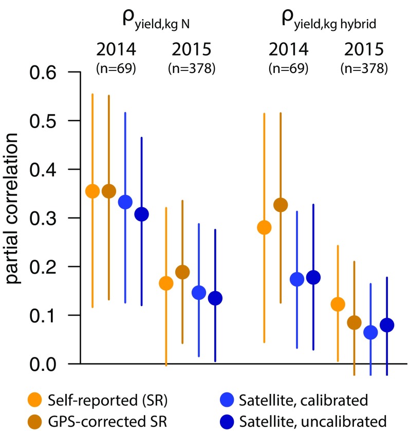
For both the 2014 and 2015 seasons, partial correlations between N use and yield are indistinguishable across satellite- and ground-based yield estimates (Fig. 4). For hybrid seed use, ground-based measures outperform satellite-based measures in 2014 but not in 2015. We interpret these results as evidence that the imperfect agreement between satellite- and ground-based yield measures shown in Figs. 2 and 3 is driven as much by noise in the ground data as it is by noise in the satellite-based estimates.

Fig. 4.

Partial correlations between input use (kilograms N or kilograms hybrid seed per acre) and yield for four different measures of yield in each study year, for fields $>$0.5 acre. Solid circles are partial correlation point estimates and lines are bootstrapped 95% confidence intervals.

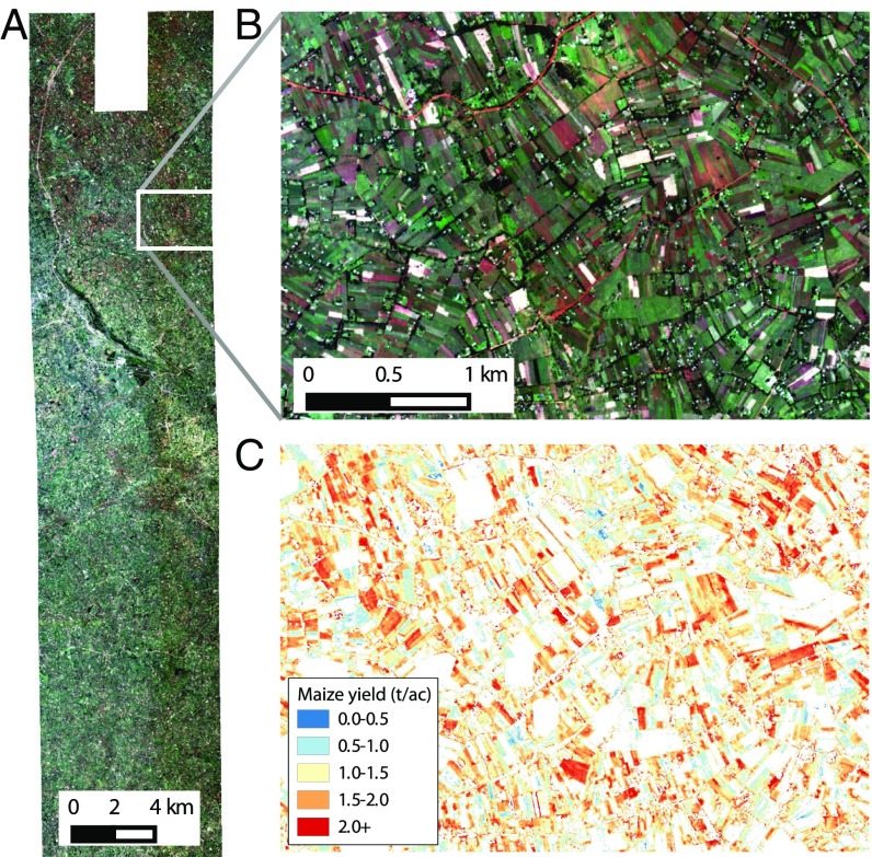
Finally, to demonstrate scalability, we develop a maize yield map of the study region for the 2015 season. This map is constructed by first using field data collected on both maize and nonmaize crops to train a crop classifier that can capably distinguish maize pixels from nonmaize ones and then using Eq. 1 to estimate yield for each pixel (Methods). The input imagery and resulting yield map for a portion of the study area are shown in Fig. 5. Plot outlines are clearly distinguishable in the yield map, with large variation in productivity visible both across and within fields. For instance, estimates from this map suggest that productivity can differ on adjacent fields by a factor of 3 or more, consistent with productivity dispersion observed in other agricultural and nonagricultural systems (19, 20) and suggestive that management differences are a key determinant in overall yield variation in the region.

Fig. 5.

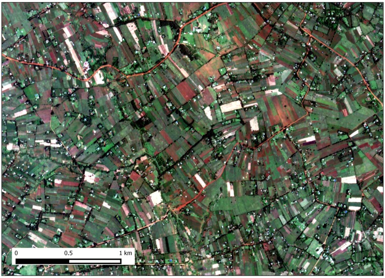
Maize yield map for the study region, 2015. (A and B) One-meter image from Terra Bella of the study region (A) and zoom-in of that image (B) (see Fig. S3 for a higher-resolution version). (C) Yield map of the zoomed-in region for pixels classified as maize.

Fig. S3.

Full-resolution version of Fig. 5B.

Discussion

Our results suggest that high-resolution satellite imagery can be used to make predictions of smallholder agricultural productivity that are roughly as accurate as survey-based measures traditionally used in research and policy applications. Furthermore, we find that a scalable uncalibrated approach to making these predictions performs almost as well as an approach that uses field data for calibration.

Our findings highlight a number of procedures for generating smallholder productivity estimates, as well as suggest future work that is needed to both improve our results and validate them in new settings. On the methodological side, we find clear evidence that vegetative indexes that capture canopy greenness outperform more traditional measures that use red reflectance in predicting maize yields, likely due to nutrient stress common in African smallholder systems. We also confirm earlier findings that farmer self-reported area is highly inaccurate (11) and find that measuring plot area with a GPS leads to important improvements in the quality of the ground data.

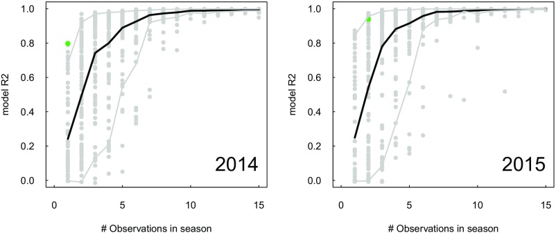
In terms of improving future predictions, obtaining more objective measures of farmer harvests, for instance through whole-field or precisely georeferenced subfield harvests conducted by survey teams, would likely improve our ability to understand the accuracy and efficacy of satellite-based measures. Such field campaigns are relatively expensive and thus have not been carried out at a reasonable scale to date, but they remain a key research priority. Obtaining more frequent imagery than the one to two cloud-free images that were acquired per growing season in our study would also be useful. As multiple high-resolution imagery providers scale up their operations, more frequent images will become available, and simulations suggest that this should substantially improve yield predictions (Fig. S2). Finally, the combination of better ground truth data and higher cadence imagery would likely help reduce current known sources of error in prediction (Fig. S1), for instance by helping to mask out noncrop features such as trees and/or helping to identify portions of plots with later season stress not apparent in early-season or midseason imagery.

Fig. S2.

Relationship between adjusted $R^2$ for a model to predict simulated yields from simulated GCVI and the number of dates of observations used in the model. Each gray circle represents a different random sample of observation dates, and solid lines show mean (black line) or 5–95% confidence interval (gray lines). Green circle corresponds to dates of actual imagery acquired in each year.

Our approach could have a range of applications for both research and policy. First, inexpensive estimates of yields at the field scale could enable better targeting of agricultural interventions and better evaluation of their impact. Many agricultural interventions—from government programs to nongovernmental organization (NGO) projects—are never evaluated, in part because of the difficulty and expense in collecting outcome data. Inexpensive field-scale productivity measures could transform the ability to conduct impact evaluations of agricultural programs, thus expanding the evidence base on the efficacy of particular interventions. Second, the ability to measure productivity on large numbers of plots over time could lead to large improvements in our ability to understand the magnitude and determinants of yield gaps. The prototype yield maps reported here suggest remarkable heterogeneity both within and across fields, and these yield maps could be used to evaluate a number of hypotheses about the sources of yield gaps even in the absence of management data (7). Finally, field-scale productivity estimates could support the development and expansion of financial products for smallholders, such as insurance products indexed to local-area–averaged yield performance or credit products where yield history is used to inform credit worthiness.

Methods

Field Data Collection.

Field campaigns were conducted in 2014 and 2015 to visit farmers’ fields within the extent of the available satellite imagery. The study area spanned a roughly 8-km wide by 50-km long region in Bungoma and Kakamega Counties, Western Province, Kenya. Maize is the main crop in this region, with planting for the main growing season occurring between March and April and harvest between August and September. Surveyed farmers were all clients of One Acre Fund, a large East African agricultural microfinance organization. Farmers were randomly selected from One Acre Fund client rosters and were visited twice in each year by survey enumerators that were hired and trained in collaboration with Innovations for Poverty Action, a research organization active in the area. The first visit occurred during the main (“long rains”) growing season 1–2 mo before harvest, and enumerators mapped plot boundaries using GPS devices and elicited information on farmer-estimated plot area, intercropping, input use, and planting date for each mapped plot. For GPS mapping we used Garmin GPSMAP64 devices with a reported 3-m accuracy. The second visit was conducted 1–2 mo after the main maize harvest (with harvest typically in early September), and data were collected on plot-specific harvest amounts. Information was collected for all maize plots grown by a household, as well as for up to two nonmaize plots.

Image Processing.

Images used in this study were acquired by Terra Bella’s Skysat sensors as part of Google’s “Skybox for Good” program and are publicly available on Google’s Earth Engine platform. Skysat sensors acquire data using three detectors, each of which obtained multiple 8 × 8-km images within our study region. To radiometrically correct the images to surface reflectance, we first manually masked out clouds and cloud shadows within individual tiles for each image and then mosaicked the tiles together, using seamless mosaicking in the ENVI (Environment for Visualizing Images) software. We then obtained Landsat surface reflectance data (via Earth Engine) for the study region for dates within 2 wk of our Skysat images and calculated histograms for each Landsat band. A pseudo-Landsat histogram for the Skysat image date was then calculated by interpolating the Landsat histograms from the nearest dates with cloud-free images, and the Skysat bands were then calibrated using histogram matching to these Landsat histograms. The NDVI (21), GCVI (22), and EVI (23) indexes were then calculated as

$$NDVI=(NIR-red)/(NIR+red)GCVI=(NIR/green)-1EVI=2.5\ast (NIR-red)/(NIR+6\ast red+7\ast blue+1).$$

For the 2014 growing season only a single relatively cloud-free image (June 17, 2014) was acquired over the study region by TerraBella sensor Skysat 1, whereas in 2015 two relatively cloud-free images (May 15 and July 3, 2015) were obtained (by Skysat 2 and 1, respectively). Flowering for maize in this region typically occurs in the last week of May or the first week of June, so that the 2014 image was acquired just before flowering for most fields, whereas the 2015 images were acquired during vegetative and early grain filling stages, respectively. The May 15, 2015 image was georeferenced in ArcMap, using manual selection of points from the Environmental Systems Research Institute basemap. Other images were then georeferenced using automated image-to-image registration in ENVI.

Yield Estimation.

Two approaches to satellite yield estimation were tested in this study. The first, “satellite, calibrated,” was a simple linear regression model that related image values of GCVI, NDVI, or EVI to field-measured yields,

$$yiel{d}_i={\beta }_0+\sum _{t=1}^N{\beta }_{t}V{I}_{it}+{\epsilon }_i,$$ [1]

where $i$ represents a specific field, $t$ is a specific image date, and $N$ is the number of image dates.

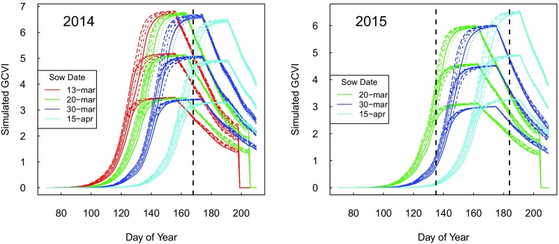
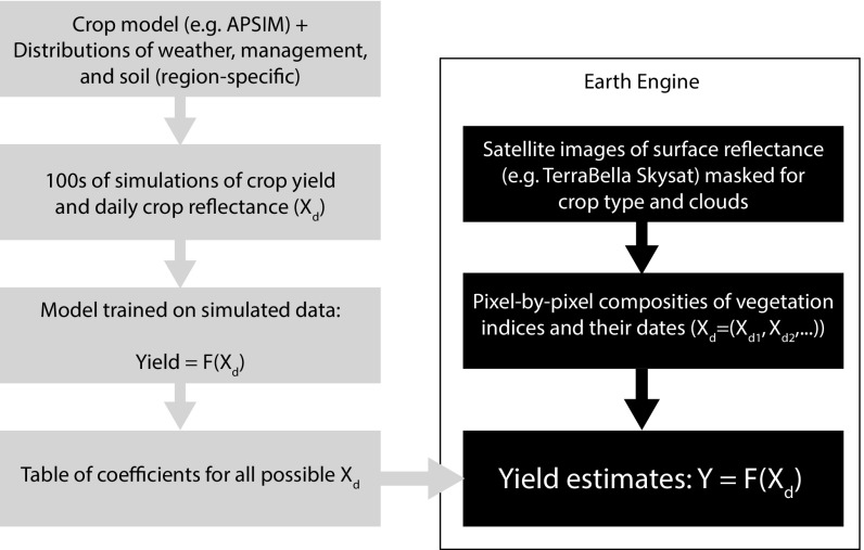
The second, “satellite, uncalibrated” approach used simulations with the Agricultural Production Systems Simulator APSIM)-Maize model to generate pseudodata for yield and VI to calibrate the values of $\beta$ in Eq. 1. We refer to this approach as “uncalibrated” because it does not rely on any field measurements of yield. Specifically, 100 simulations for different levels of fertilizer rates, sowing dates, planting densities, and initial soil moisture were simulated for each study year to generate variability in crop growth and yields, and then daily GCVI was calculated based on published relationships between GCVI and total canopy nitrogen (24). The cultivar Hybred511 within APSIM was used for all simulations, as it results in a phenology typical of maize in the region, and soils were defined based on a predefined soil within APSIM for the Katumani, Kenya research station, which had an available water holding capacity of 164 mm. A separate model was developed for each year based on the simulations using weather for that year, where weather was obtained for a nearby weather station in Kakamega, using NASA POWER (http://power.larc.nasa.gov/) for solar radiation and for days missing temperature or rainfall. In addition, although we simulated a wide range of sow dates (from March 1 to April 15), for each year the regressions used only simulations with sow dates starting after the main onset of rains (eliminating sowings before March 13 in 2014 and March 20 in 2015), so as not to calibrate the model with unrealistic sow dates. The simulated time series of GCVI for each year, along with the dates used to predict yields, are shown in Fig. S4, and a schematic overview of the procedure is shown in Fig. S5.

Fig. S4.

Simulated time series of canopy GCVI for each year for different management combinations, based on the APSIM-maize model. Colors represent different potential sow dates in each year, and individual lines represent different potential management combinations for that sow date. Vertical dashed lines show timing of actual images used for yield prediction.

Fig. S5.

Schematic overview of the procedure for generating and mapping uncalibrated yield estimates. Each box represents a specific step in the process, with boxes colored black implemented in Google Earth Engine.

Yield Responses to Inputs.

To relate self-reported and satellite-estimated yields to input use (Fig. 4), we estimated standard log–log production functions, modeling the log of yields as a function of log kg of inorganic N applied per acre, log kg of hybrid seed applied per acre, and log acreage; i.e.,

$$log(yiel{d}_i)={\lambda }_0+{\lambda }_{1}log(N_i)+{\lambda }_{2}log(hy{b}_i)+{\lambda }_{3}log(are{a}_i)+{\epsilon }_i.$$ [2]

The regression was estimated separately for each yield measure, with partial correlations of each input to each of the different yield measures reported in Fig. 4. Farmer-reported acreage was used for the SR estimates; all other estimates used GPS-estimated area.

Crop Classification and Maize Yield Mapping.

Yields were mapped for each pixel, using the calibrated model from Eq. 1. A land cover classification mask was then created for 2015 using May 15, July 3, and September 16 Skysat imagery as input into random forests, a method widely used for land cover mapping (25). The September 16 image postdates the maize harvest in our study region but is useful for land cover classification, as other common crops in the region such as sugarcane remain unharvested and thus distinguishable in imagery. The random forest classifier was trained using locations of individual crops collected in the field, as well as visual identification of trees and urban areas in the imagery. Training accuracy was 86%. The yield estimates were then masked for pixels not classified as maize, resulting in the map shown in Fig. 5.

References

- 1.World Bank . World Development Report - “Agriculture for Development”. The International Bank for Reconstruction and Development/The World Bank; Washington, DC: 2008. [Google Scholar]
- 2.Carletto C, Jolliffe D, Banerjee R. From tragedy to renaissance: Improving agricultural data for better policies. J Dev Stud. 2015;51(2):133–148. [Google Scholar]
- 3.Carletto G, et al. 2010 Improving the Availability, Quality and Policy-Relevance of Agricultural Data: The Living Standards Measurement Study – Integrated Surveys on Agriculture, Third Wye City Group Global Conference on Agricultural and Rural Household Statistic (Food and Agricultural Organization of the United Nations, Rome). http://www.fao.org/fileadmin/templates/ess/pages/rural/wye_city_group/2010/May/WYE_2010.2.1_Carletto.pdf. Accessed September 26, 2016.
- 4.Duflo E, Kremer M, Robinson J. How high are rates of return to fertilizer? Evidence from field experiments in Kenya. Am Econ Rev. 2008;98(2):482–488. [Google Scholar]
- 5.Emerick K, de Janvry A, Sadoulet E, Dar MH. Technological innovations, downside risk, and the modernization of agriculture. Am Econ Rev. 2016;106(6):1537–1561. [Google Scholar]
- 6.Frelat R, et al. Drivers of household food availability in sub-Saharan Africa based on big data from small farms. Proc Natl Acad Sci USA. 2016;113(2):458–463. doi: 10.1073/pnas.1518384112. [DOI] [PMC free article] [PubMed] [Google Scholar]
- 7.Lobell DB. The use of satellite data for crop yield gap analysis. Field Crop Res. 2013;143:56–64. [Google Scholar]
- 8.van Ittersum MK, et al. Yield gap analysis with local to global relevance—A review. Field Crop Res. 2013;143:4–17. [Google Scholar]
- 9.Farmaha BS, et al. Contribution of persistent factors to yield gaps in high-yield irrigated maize. Field Crop Res. 2016;186:124–132. [Google Scholar]
- 10.Roy DP, et al. Landsat-8: Science and product vision for terrestrial global change research. Rem Sens Environ. 2014;145:154–172. [Google Scholar]
- 11.Carletto C, Gourlay S, Winters P. From guesstimates to GPStimates: Land area measurement and implications for agricultural analysis. J Afr Econ. 2015;24(5):593–628. [Google Scholar]
- 12.Belward AS, Skøien JO. Who launched what, when and why; trends in global land-cover observation capacity from civilian earth observation satellites. ISPRS J Photogramm Remote Sens. 2015;103:115–128. [Google Scholar]
- 13.Lobell DB, Thau D, Seifert C, Engle E, Little B. A scalable satellite-based crop yield mapper. Rem Sens Environ. 2015;164:324–333. [Google Scholar]
- 14.Fermont A, Benson T. Estimating Yield of Food Crops Grown by Smallholder Farmers. International Food Policy Research Institute; Washington, DC: 2011. pp. 1–68. [Google Scholar]
- 15.Tittonell P, Vanlauwe B, De Ridder N, Giller KE. Heterogeneity of crop productivity and resource use efficiency within smallholder Kenyan farms: Soil fertility gradients or management intensity gradients? Agr Syst. 2007;94(2):376–390. [Google Scholar]
- 16.Gitelson AA, Vina A, Ciganda V, Rundquist DC, Arkebauer TJ. Remote estimation of canopy chlorophyll content in crops. Geophys Res Lett. 2005 doi: 10.1029/2005GL022688. [DOI] [Google Scholar]
- 17.Bausch WC, Halvorson AD, Cipra J. Quickbird satellite and ground-based multispectral data correlations with agronomic parameters of irrigated maize grown in small plots. Biosystems Eng. 2008;101(3):306–315. [Google Scholar]
- 18.Marenya PP, Barrett CB. State-conditional fertilizer yield response on western Kenyan farms. Am J Agric Econ. 2009;91(4):991–1006. [Google Scholar]
- 19.Hsieh CT, Klenow PJ. Misallocation and manufacturing TFP in China and India. Q J Econ. 2009;124(4):1403–1448. [Google Scholar]
- 20.Lobell DB, Cassman KG, Field CB. Crop yield gaps: Their importance, magnitudes, and causes. Annu Rev Environ Resour. 2009;34(1):179–204. [Google Scholar]
- 21.Rouse JW, Haas RH, Schell JA, Deering DW. Monitoring vegetation systems in the great plains with ERTS. In: Freden SC, Mercanti EP, Becker MA, editors. Third ERTS Symposium. Vol. 1. NASA; Washington, DC: 1974. pp. 309–317. [Google Scholar]
- 22.Gitelson AA, et al. Remote estimation of leaf area index and green leaf biomass in maize canopies. Geophys Res Lett. 2003;30(5):1248. [Google Scholar]
- 23.Huete A, et al. Overview of the radiometric and biophysical performance of the MODIS vegetation indices. Rem Sens Environ. 2002;83(1):195–213. [Google Scholar]
- 24.Schlemmer M, et al. Remote estimation of nitrogen and chlorophyll contents in maize at leaf and canopy levels. Int J Appl Earth Obs Geoinf. 2013;25(1):47–54. [Google Scholar]
- 25.Rodriguez-Galiano VF, Ghimire B, Rogan J, Chica-Olmo M, Rigol-Sanchez JP. An assessment of the effectiveness of a random forest classifier for land-cover classification. ISPRS J Photogramm Remote Sens. 2012;67:93–104. [Google Scholar]