Significance
Different interaction rules among animals can produce patterns of collective motion similar to those observed in bird flocks or fish schools. To help distinguish which rules are implemented in animal collectives, we studied the birth of the interaction rule in zebrafish during development from hatching to the juvenile stage. We used newly developed machine vision algorithms to track each animal in a group without mistakes. A weak attraction starts after hatching and gets stronger every day during development. Attraction consists in each larva moving toward one other larva chosen effectively at random and then switching to another one. This rule, simply by statistics, makes each individual move to regions of high density of individuals to produce collective motion.
Keywords: collective behavior, interaction rule, zebrafish, development, shoaling
Abstract
The striking patterns of collective animal behavior, including ant trails, bird flocks, and fish schools, can result from local interactions among animals without centralized control. Several of these rules of interaction have been proposed, but it has proven difficult to discriminate which ones are implemented in nature. As a method to better discriminate among interaction rules, we propose to follow the slow birth of a rule of interaction during animal development. Specifically, we followed the development of zebrafish, Danio rerio, and found that larvae turn toward each other from 7 days postfertilization and increase the intensity of interactions until 3 weeks. This developmental dataset allows testing the parameter-free predictions of a simple rule in which animals attract each other part of the time, with attraction defined as turning toward another animal chosen at random. This rule makes each individual likely move to a high density of conspecifics, and moving groups naturally emerge. Development of attraction strength corresponds to an increase in the time spent in attraction behavior. Adults were found to follow the same attraction rule, suggesting a potential significance for adults of other species.
Collective animal behavior is studied with increasing detail in natural habitats (1–6) and laboratory conditions (7–14). Local interactions among animals can, in many cases, explain these patterns of collective behavior, and a variety of interaction rules have been proposed (7, 8, 11, 14–27).
One of the technical problems in discriminating among possible interaction rules is the difficulty of obtaining high-quality experimental data (25). We reasoned that the ontogeny of attraction behavior offers a unique opportunity to obtain a large high-quality dataset. This dataset should constrain the space of possible models to those that can explain interactions every day during development.
We turned to zebrafish, Danio rerio, a species in which larvae seem not to attract each other after hatching but that develop shoaling and schooling behavior during the first month of development (12, 14, 28–33). Our choice was based on our previous work in the adult suggesting a simplicity of the rules compared with other species (14).
In this work, we follow the formation of attraction behavior during the ontogeny of collective behavior in zebrafish. We used our newly developed tracking system of animals in groups, idTracker (34), in a total of 524 videos for the study of development and videos for adults. We found that zebrafish are very weakly attracted to each other by 7 days postfertilization (dpf), and the attraction gets stronger each day during development. By 9 dpf, larvae are likely found close to each other, and, by 15 dpf, it is common to see animals moving in groups. Analysis and modeling of the developmental dataset point to attraction as turning toward a randomly chosen conspecific. Using this simple rule, animals are more likely to move toward high density of conspecifics without lumping, and group movement emerges. Development is found to correspond to an increasingly large amount of time spent in interaction behavior. We also found that the same rule can explain the behavior of freely moving adults, suggesting a potential significance for other species.
Results
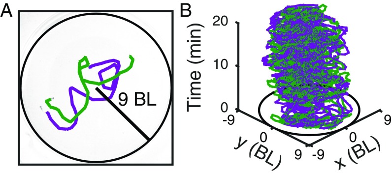
We video-recorded isolated zebrafish and groups of two, four, or seven in an arena of 9 to 10 bodylengths (BL) of radius every day from 7 dpf, in which they start to swim, until 24 dpf (Fig. 1A; see Fig. S1A for setup). We used idTracker (34) to obtain the trajectory of each animal in a group using a method of image fingerprinting without the need for manual corrections (Fig. 1B). Correct identification of individuals is necessary for tests at the individual level but also to obtain the correct values of quantities derived from trajectory data like velocities or accelerations.
Fig. 1.
Setup and tracking. (A) Setup of 9 to 10 BL radius. (B) Example of trajectory data for two zebrafish obtained from video using idTracker (34).
Fig. S1.
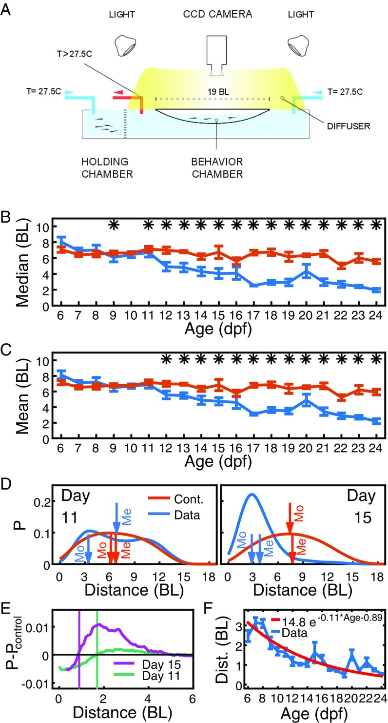
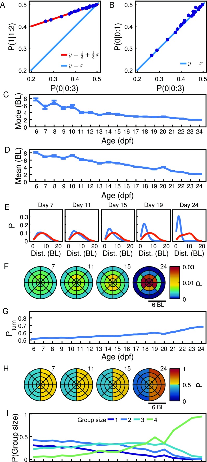
Setup, measuring interindividual distance and repulsion radius. (A) Experimental setup. (B) Median distance at ages 6 dpf to 24 dpf, averaged over 4 to 12 pairs of fish (blue) and control randomized data (orange). Error bars are SEM, *P < 0.05. (C) Same as B but for the mean distance. (D) Example distribution of interindividual distances for single trials on days 11 (left, blue) and 15 (right, blue), and the respective distributions from control randomized data (orange). Arrows indicate the mean (Me) and the mode (Mo). (E) Difference of distributions of distances and their controls for 11 dpf and 15 dpf. Vertical lines indicate the respective zero crossing. (F) Position of the zero crossing in the difference of distance distributions as shown in E at ages 6 dpf to 24 dpf (blue) and exponential fit (red). For E and F, distributions were obtained using kernel density estimation with an Epanechnikov kernel and a bandwidth of BL. Error bars are SEM. (All data are from group size two animals.)
Ontogeny of Collective Behavior in Zebrafish.
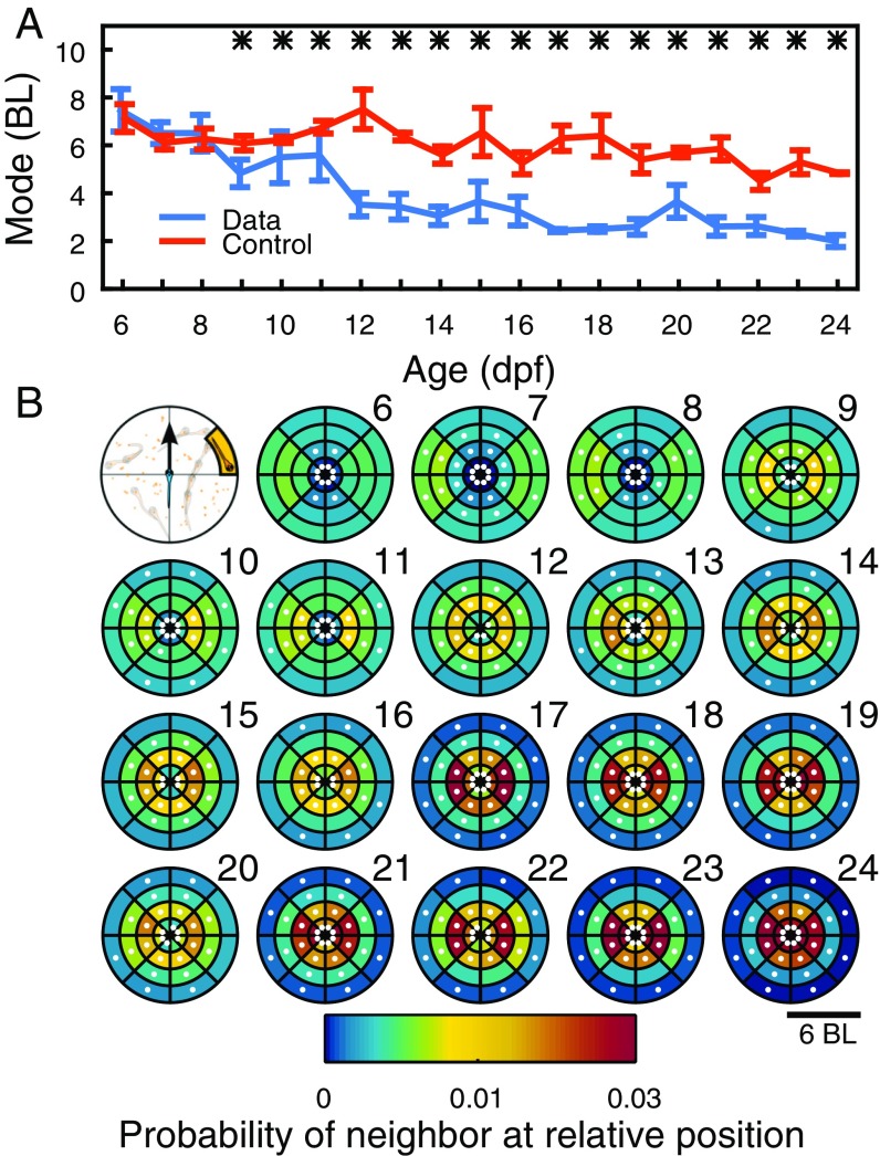
We first analyzed experiments that used pairs of zebrafish. A simple measure of whether two animals are interacting is given by their distance apart. We found that the most likely distance, or mode, is significantly lower than control randomized data from 9 dpf (Fig. 2A). The median distance is significant from 11 dpf (Fig. S1B), and the mean distance is significant from 12 dpf (Fig. S1C); this is because the distributions of distances are asymmetric, and the mode separates better data from control early in development (Fig. S1D).
Fig. 2.
Development of distance and relative position between two fish. (A) Most likely distance between pairs of fish at ages 6 dpf to 24 dpf (blue), N = 4 to 12 pairs per day, and same for control randomized data (orange). Data are mean SEM. Stars indicate . (B) Focal animal is at the center of the coordinate system, with velocity vector pointing in the direction of y axis (top left). Other images show probability of finding second animal in space for ages 6 dpf to 24 dpf. Data are mean for each age, with age indicated by numbers 6 to 24. Dots indicate regions with .
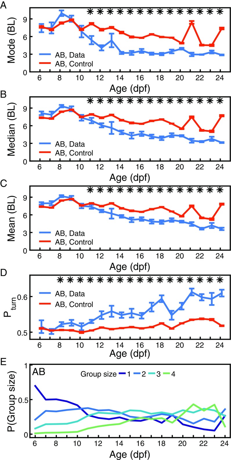
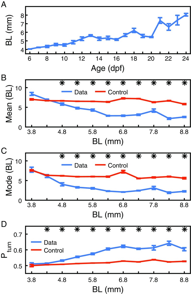
We obtained similar results in the AB zebrafish strain, but significance in mode, median, and mean distance start from 11 dpf (Fig. S2). Also, the analysis can be given in terms of fish BL instead of age (Fig. S3).
Fig. S2.
Results for the AB strain. (A) Most likely distance or mode computed from 4 to 12 pairs of AB zebrafish at ages 6 dpf to 24 dpf (blue). Same is shown for control randomized data (orange). Error bars are SEM. *P < 0.05. (B) Same as A, but for the median. (C) Same as A, but for the mean. (D) Probability of accelerating toward the side on which the other animal of the pair is located, for experimental (blue) and control data (orange) at ages 6 dpf to 24 dpf. Error bars are SEM. *P < 0.05. (E) Probability of finding groups of one, two, three, or four individuals at less than 6 BL in a group of individuals, defined as the probability of a focal having , , , and neighbors at a distance of less than 6 BL.
Fig. S3.
Development of distance and attraction versus BL. (A) BL at 6 dpf to 24 dpf. Error bars are SEM. (B) Mean distance computed from 2 to 19 pairs of fish with BL 3.8 mm to 8.8 mm (blue). Same is shown for control randomized data (orange). Error bars are SEM. *. (C) Same as B, but for the most likely distance. (D) Probability of accelerating toward the side on which the other animal in the pair is located (blue) and control randomized data (orange) for BL 3.8 mm to 8.8 mm. Error bars are SEM. Stars indicate days with .
Interactions may depend not only on the distance between animals but also on the relative positions in space. Relative positions were studied using a coordinate system with origin on the focal animal and positive y axis pointing in the direction of its velocity vector (Fig. 2B, top left). We then computed the probability of finding the second animal in space (Fig. 2B; numbers indicate age). At 7 dpf to 11 dpf, animals spend significantly more time side by side than in front/back positions, and during 12 dpf to 24 dpf, they spend increasingly more time close to each other. Around the focal animal, there is also a region of low probability of finding the second animal (Fig. S1E). This region reduces size during development (Fig. S1F).
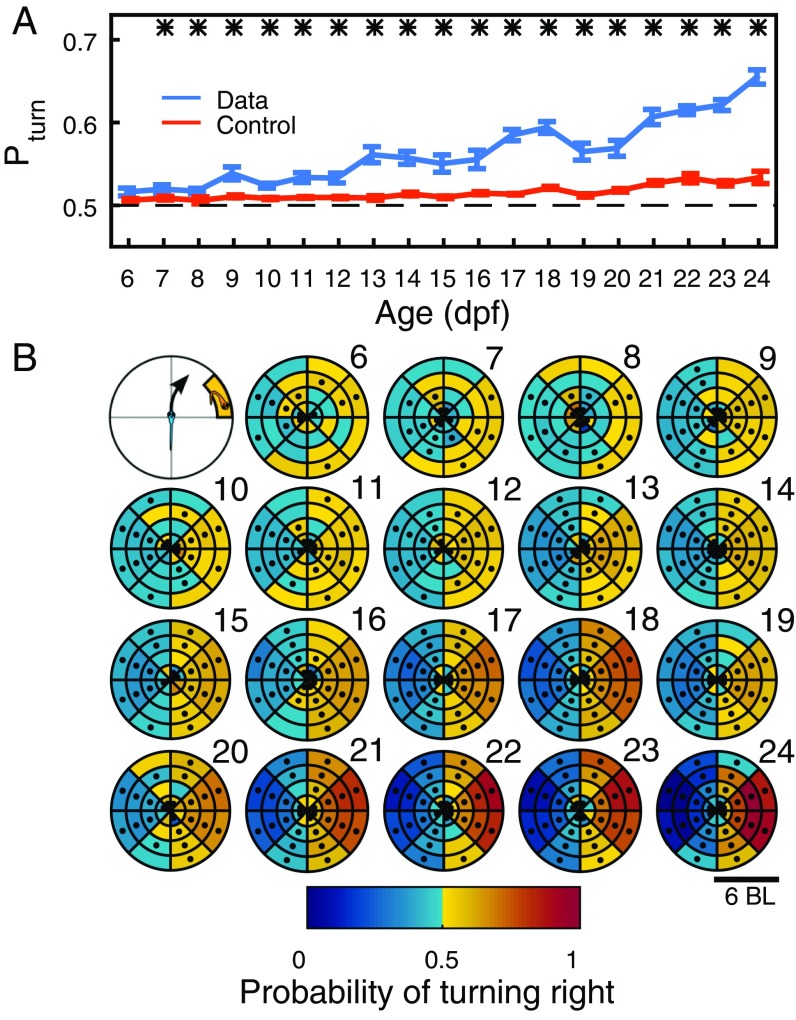
Distance and relative positions do not directly distinguish whether animals repel or attract each other. Attraction and repulsion can be studied more directly by measuring whether an individual accelerates toward or away from another individual (9, 10). As acceleration values change during development also for nonsocial interactions, we found it more useful to compute the probability of accelerating toward particular places. Specifically, we computed the probability () that the focal turns to the side where the other fish is. This probability is significant from 7 dpf and increases during development (Fig. 3A). For the AB zebrafish strain, significance starts from 8 dpf (Fig. S2D).
Fig. 3.
Development of attraction. (A) Probability of accelerating toward the side in which the other animal in the pair is located (blue), and control randomized data (orange) from 6 dpf to 24 dpf. Data are mean, and error bars are SEM. Stars indicate days with . (B) Probability of focal animal turning right when second animal is in different positions in space. Focal animal is at the center of the coordinate system, with velocity vector pointing in the direction of y axis. Data are mean for each age, with age indicated by numbers 6 to 24. Dots indicate regions with .
More detail about attraction can be obtained studying the probability of turning to the right side depending on the location of the second animal (Fig. 3B). For 24 dpf, for example, the focal animal more often accelerates to the right (left) when the other animal is at its right (left) (Fig. 3B, day 24). This attraction structure starts to be significant at 6 dpf to 7 dpf and gets stronger during development (Fig. 3B).
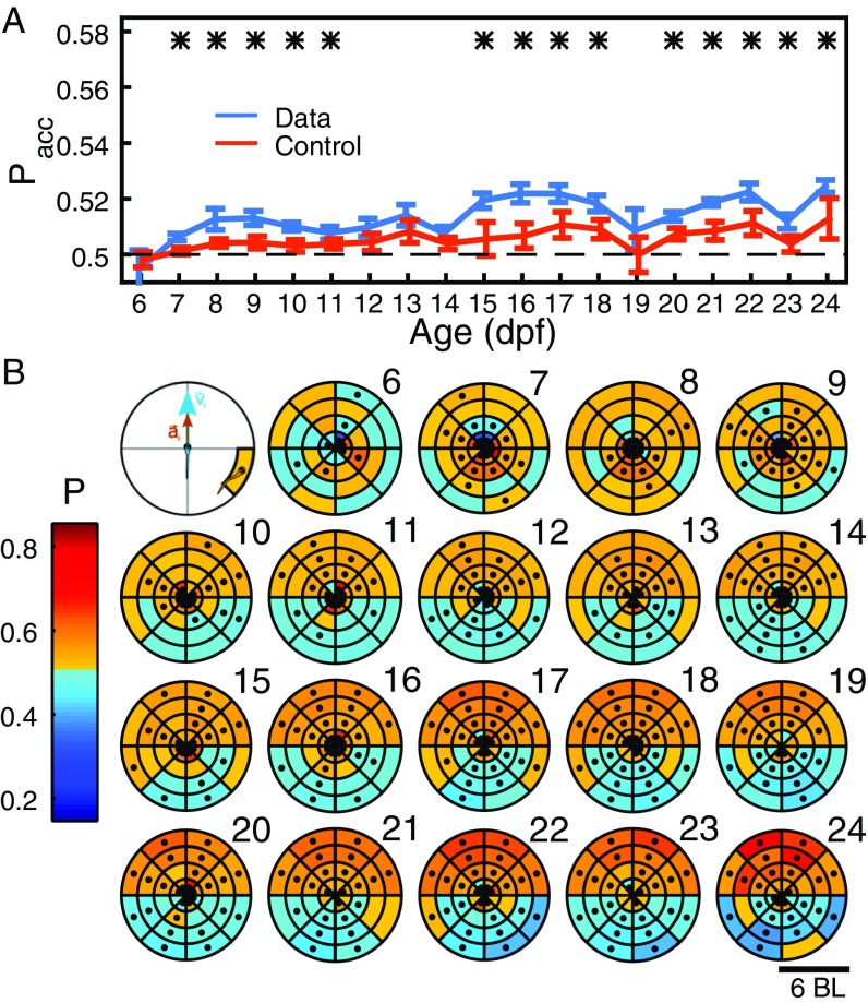
Attraction can also be studied to the front or back position (Fig. S4), giving that, at 10 dpf to 24 dpf, animals accelerate to another animal in front and brake when behind, and, at 6 dpf to 9 dpf, there is some repulsion from an animal behind (Fig. S4B).
Fig. S4.
Attraction to a neighbor behind/in front. (A) Probability of speeding up/slowing down when the neighbor is in front/behind, for experimental (blue) and control data (orange) for 6 dpf to 24 dpf. Error bars are SEM. *P < 0.05. (B) Probability of the focal animal speeding up when the second animal is in different positions in space for ages 6 dpf to 24 dpf. Focal animal is at the center of the coordinate system, with velocity vector pointing in the direction of y axis. Dots indicate regions with P < 0.005.
Using Development to Extract the Rule of Attraction.
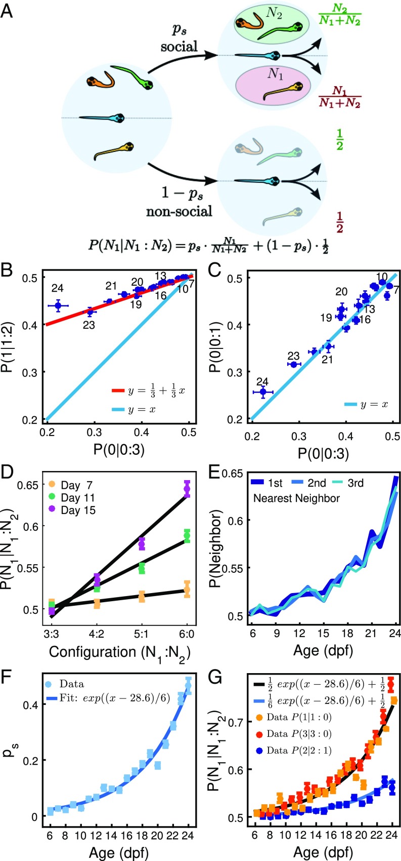
We used experiments with four fish to find whether there is an attraction rule that can explain the data. We found best correspondence by a model in which each animal interacts a proportion of the time by moving toward a randomly chosen individual (Fig. 4A). According to this model, when a focal has animals to one side and animals to the other, the probability of choosing the side with animals would be given by
| [1] |
and for the other side. This probability has two contributions. The first contribution comes from the proportion of time spent in interactions in which the focal chooses one animal at random and thus the side with animals with probability . The second contribution comes from the remaining proportion of time, , in which the focal does not interact with other animals, giving, in our experiments, in which no consistent left–right asymmetry exists, a probability for each side.
Fig. 4.
Attraction rule from developmental data. (A) Diagram of model in which individuals spend a proportion of time in interactions consisting in turning toward one animal chosen at random and time not interacting. Probability of moving to the side with animals is then Eq. 1. (B) Relationship between the probability of turning to the side of animal in a configuration (1:2), , and the probability of turning to the side of no animals in a configuration (0:3), . Blue dots indicate experimental data, with numbers indicating age in dpf. Red line indicates theoretical line in Eq. 2. (C) Relationship between turning to the side of no animals in experiments with two and four fish, vs. . Blue dots indicate experimental data, with numbers indicating age in dpf. Blue line indicates theoretical line in Eq. 3. (D) Probability of turning to side with three, four, five, and six animals in a group of seven animals for days , and . (E) Probability that the side chosen by an animal corresponds to the closest, intermediate, or farthest neighbor. (F) Parameter as extracted fromthe data (dots) and fit to an exponential (line). (G) Probabilities , , and during development. Lines are Eqs. 4 and 5.
The model in Eq. 1 has one parameter, the time spent in interactions, , but also makes predictions independent of this parameter. For experiments using four animals, a focal fish can be found with zero and three fish to its sides (configuration 0:3) or one and two fish (configuration 1:2). The model predicts a relationship between the probabilities for these two configurations that is independent of the parameter as
| [2] |
plotted as a solid red line in Fig. 4B. Another relationship is the one between the probability of turning to the side of no animals for these experiments with four animals and those experiments with only two animals as
| [3] |
plotted as a solid blue line in Fig. 4C. The general parameter-free relationship between two probabilities can be found in Methods.
We checked that these theoretical predictions in Eqs. 2 and 3 are also seen in agent-based simulations in which each agent turns with probability to the side of another agent chosen at random and, with probability , turns left or right randomly (Fig. S5B, dots for different values of ; see Methods for details of simulations).
Fig. S5.
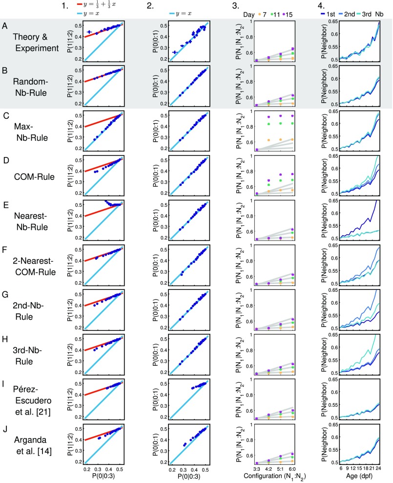
Comparison of agent-based simulations implementing different interaction rules. Columns show: 1, versus ; 2, versus ; 3, the probability of turning to the side with three, four, five, and six animals in a group of seven animals; and 4, the probability that the nearest, second-, and third-nearest neighbor is at the side the focal is turning to. (A) Results from theory and experiments (repeated from Fig. 4 B–E). (B) Results from the rule “choose neighbor randomly and turn toward it” presented in Agent-Based Modeling. For the remaining rules, the side to turn to is determined by (C) the majority of neighbors, (D) the center of mass (mean position) of all neighbors, (E) the nearest neighbor, (F) the mean position of the two nearest neighbors, (G) the second-nearest neighbor, (H) the third-nearest neighbor, (I) the probability given by equation 17 from Pérez-Escudero et al. (21) with s = 1.50, and (J) the probability given by equation 3 from Arganda et al. (14) with a = 6.70, s = 6.13, and k = 0.17. Rules in C–E do not agree with theory and experiments in conditions shown in columns 1 through 3; rules in F–H differ in column 4. For I and J, nonlinear least-square optimization was used to find the parameter values that most favorably fit conditions 1 through 3.
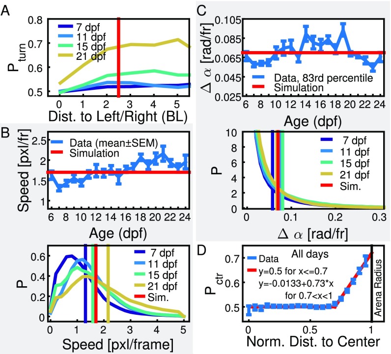
For the analysis of the experimental data, we realized that the probability of turning to one side is random when another animal is very close, increases with the distance to another animal, and, at BL, is independent of distance (Fig. S6A). As for this first analysis we are not considering space dependencies of attraction, we used only data when animals are at BL from the focal. We found that these experimental data correspond well with the theoretical predictions in Eq. 2 (Fig. 4B) and Eq. 3 (Fig. 4C), with different days marked with corresponding numbers.
Fig. S6.
Extraction of parameter values for simulation. (A) Probability of an animal turning toward its conspecific versus interindividual distance for 7, 11, 15, and 21 dpf. The horizontal red line indicates the radius of reduced attraction = 2.5 BL used in the simulations and for filtering close neighbors in Fig. 4. (B) (Top) Average mean speed for each day. The horizontal red line indicates the step width chosen for simulations (s = 1.7 pixels per frame). Error bars are SEM. (Bottom) Distribution of speed for 7, 11, 15, and 21 dpf. Vertical lines indicate the mean. Distributions are unimodal, and the average mean as indicated by the vertical red line is chosen in simulations. (C) (Top) Average over the 83rd percentile of the turning angles for each day. Error bars are SEM. The horizontal red line indicates the angle used in the simulations ( = 0.07 rad per frame). (Bottom) Distribution of turning angles for 7, 11, 15, and 21 dpf. Distributions decrease continuously, and, for simulations, we choose a value that coincides with the 83rd percentile, as indicated by the vertical red line. (D) Average probability of an animal turning toward the center of the arena versus its normalized distance to the center. The red line indicates the approximation used in the simulations. Data of all age groups were pooled together. (Group size in A–C is two fish; group size in D is one fish.)
Another prediction of the interaction rule in Eq. 1 is that the probability of turning to the side with animals grows linearly with as . Groups of four animals only have two possible configurations, and , so, for a proper test of this linearity, we used the four configurations arising in groups of seven fish (Fig. 4D).
We also checked that animals do not favor turning toward the side with the closer, intermediate, or farthest neighbor. The probability that the side chosen is the one with the closest animal is found to be very similar to the probability that it is the side with the animal at intermediate distance or the side with the farthest animal during all development (Fig. 4E). Our agent-based simulations with agents turning to another randomly chosen agent also give this result (Fig. S5B, column 4).
We simulated alternative agent-based models with one of eight other interaction rules, including turning to the side with more animals (Fig. S5C), to the side of the center of mass of the rest of the group (Fig. S5D), to the closest animal (Fig. S5E), to the center of mass of the two closest neighbors (Fig. S5F), to the second neighbor (Fig. S5G), and to the third neighbor (Fig. S5H), and using the nonlinear decision rules from ref. 14 (Fig. S5J) and ref. 21 (Fig. S5I). We found worse correspondence with experimental data using any of these eight rules in Fig. S5C–J than the theoretical predictions from Eq. 1 (Fig. S5A) or its implementation with agents turning toward one animal chosen at random (Fig. S5B).
N1 Using the Attraction Rule for a Quantitative Description of Development.
Once we tested the parameter-free predictions of the model, we used its “attraction” parameter in Eq. 1 to give a compact description of changes during development. For each day , we computed three values for by fitting Eq. 1 to the experimental probabilities , , and of that day and computed its mean value (Fig. 4F, dots). The value of the attraction parameter increases rapidly during development and could be fitted for the period 6 dpf to 24 dpf with the exponential (Fig. 4F, line).
Inserting into Eq. 1, one obtains that the change during development of the different probabilities obtained in groups of two and four fish is expected to be of the form
| [4] |
| [5] |
These expressions correspond well with the experimental development of the probabilities , , and (Fig. 4G).
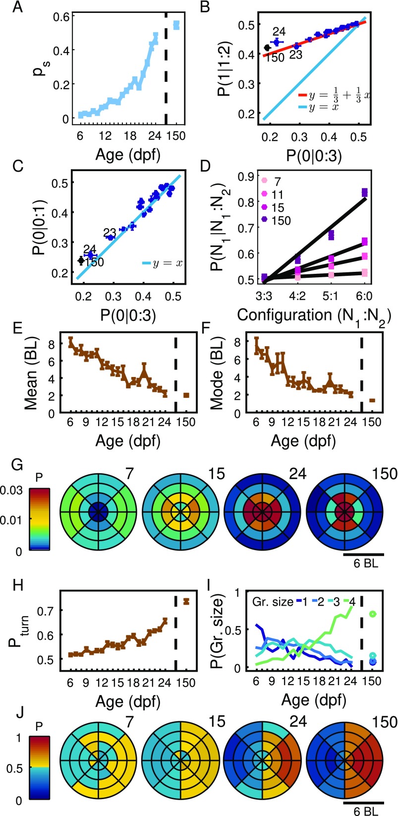
We also performed experiments on adult zebrafish of 150 dpf to assess how developed interactions are by 24 dpf. For example, the attraction parameter increases exponentially from a value of at 6 dpf to a value of at 24 dpf, but only has a very small increase to a value of in the adult stage of dpf (Fig. S7A). The other parameters measuring interaction also have values at dpf close to those at dpf (Fig. S7).
Fig. S7.
Comparison with results for adult zebrafish. Results for ages 6 dpf to 24 dpf are repeated from the main text. (A) Parameter extracted from data for groups of two and four fish. (B) Relationship between and during development, with numbers indicating 23, 24, and 150 dpf. Red line shows Eq. 3 from main text, . Line (blue) is given as reference. (C) Probability of turning to the side with no animals in experiments with four animals, , versus the same probability in experiments with pairs, (blue dots, numbers indicate 23, 24, and 150 dpf). Blue line is . (D) Probability of turning to side with three, four, five, and six animals in a group of seven animals for 7, 11, 15, and 150 dpf. (E) Mean distance between pairs of fish at ages 6 dpf to 24 dpf and 150 dpf, N = 4 to 12 per day. Error bars are SEM. (F) Same as E but for the most likely distance. (G) Probability of finding second animal in space for ages 7, 15, 23, and 150 dpf. Focal animal is at the center of the coordinate system, with velocity vector pointing in the direction of the y axis. (H) Probability of turning toward the side (left or right) on which the other animal in the pair is located from 6 dpf to 24 dpf and 150 dpf. Error bars are SEM. (I) For groups of four individuals, probability of finding zero, one, two, or three individuals at less than 6 BL, corresponding to a group size of one to four animals. (J) Probability of focal animal turning right when second animal is in different positions in space in the same coordinate system as in G.
Agent-Based Modeling.
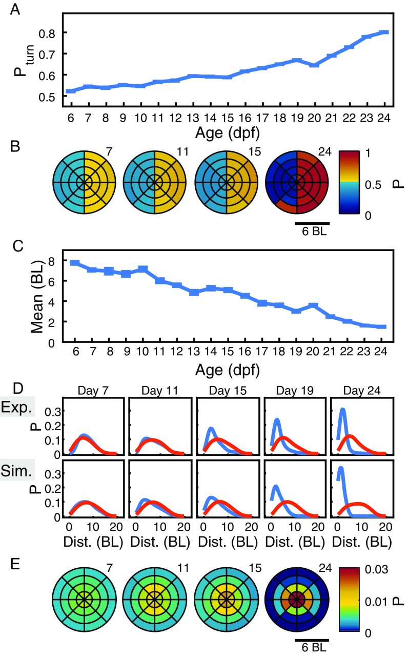
We used the agent-based model to test further the ability of the attraction rule in Eq. 1 to explain experiments. Agents turn in the direction of a randomly chosen neighbor with probability (taking values from Fig. 4F), whereas, with probability , they choose randomly to turn left or right. As the model was designed to describe the turning dynamics, we expected that turning properties would correspond well to experiments (Fig. S8A and B).
Fig. S8.
Additional results for agent-based simulation. (A) Probability of turning to the side on which the other agent is located for simulations of pairs with parameter values corresponding to 6 dpf to 24 dpf. (B) Probability of focal agent turning to the right when the second agent is in different positions in space. Focal agent is at the center of the coordinate system, with velocity vector pointing in the direction of the y axis. (C) Mean distance between agents in pairs at ages 6 dpf to 24 dpf, N = 8 pairs per day. Error bars are SEM. (D) Distributions of interindividual distances in a pair for experiment and simulation. Average distributions for 7, 11, 15, 19, and 24 dpf from experimental results obtained from four to seven trials (Top, blue) and from simulations (Bottom, blue), and the respective results from randomized control data (orange). (E) Probability of finding second animal in space with focal animal at the center of the coordinate system, with velocity vector pointing in the direction of y axis.
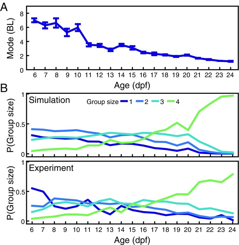
We also expected that agents would come together, and more so the higher the value of . It is less obvious that the model can give a quantitative description of aggregation properties, as these could depend on other factors apart from the turning properties. However, the match between simulations and experiments was found to be quantitative for the most likely distance between two fish (Fig. 5A), their mean distance (Fig. S8C), the distributions of distances (Fig. S8D), and the relative positions (Fig. S8E).
Fig. 5.
Aggregation from agent-based simulations. (A) Most likely distance or mode between pairs of agents at ages 6 dpf to 24 dpf (blue), N = 8 pairs per day. Data are mean, and error bars are SEM. (B) For individuals, probability of finding groups of one, two, three, or four individuals at less than 6 BL, for simulations and experiments. See Methods for details of simulations.
We also tested for the formation of groups of different sizes, defined by how many animals are together at a distance, say, of less than 6 BL. Simulations predicted, for example, that it is only from dpf that the most common group configuration in experiments with four animals should be groups of (Fig. 5B, Top), and this is also seen in experiments (Fig. 5B, Bottom).
Finally, we used simulations to test interaction models more complex than Eq. 1. We had seen in the data that attraction depends on distance to another fish for a distance less than BL (Fig. S6A), but we ignored it in our analysis using Eq. 1. A second feature seen in experiments is some repulsion from behind the focal animal (Fig. S4B), and, again, this was ignored in our analysis using Eq. 1. Simulations including these two additional features gave results very similar to those of the simpler version (Fig. S9).
Fig. S9.
Agent-based simulation with extracted attraction rule, reduced attraction at close distances, and repulsion behind the focal agent. (A) Relationship between and . Blue line is , and orange line is . (B) Probability of turning to the side with no agent in simulations with pairs, , versus the same probability in simulations with four agents, (blue dots). Blue line is . (C) Most likely distance between agents in pairs at ages 6 dpf to 24 dpf. Error bars are SEM. (D) Same as C but for the mean distance. (E) Distributions of interindividual distances in a pair. Average distributions for 7, 11, 15, 19, and 24 dpf (blue) and the respective results from randomized control data (orange). (F) Probability of finding second agent in space with focal agent at the center of the coordinate system, with velocity vector pointing in the direction of y axis. (G) Probability of accelerating toward the side on which the other agent in the pair is located. (H) Probability of focal agent turning right when second agent in the pair is in different positions in space. (I) For groups of four individuals, probability of finding zero, one, two, or three neighbors at less than 6 BL, corresponding to a group size of one to four agents. All results in A–I are averaged over N = 8 pairs per day.
Discussion
Attraction among zebrafish was found to start at 7 dpf; by 9 dpf, they are likely found close to each other, and, by 2 weeks, they swim in groups.
We used this dataset of development of interactions to test the parameter-free predictions of a model according to which animals spend part of the time in interactions with conspecifics by turning toward an animal chosen at random. The interaction rule makes each animal likely initiate motion toward a high density of animals.
We also found that our proposed rule corresponds well to adult behavior in our freely moving experiments (Fig. S7), even better than a rule we had previously obtained specifically for adult zebrafish (Fig. S5J). We thus suggest that our rule may be relevant in other species.
An important element of our rule in Eq. 1 is that each animal is not interacting at all times. The only parameter of our rule is , which measures the probability of interaction. At dpf, the ps value is very close to zero (Fig. 4F), and this translates into animals spending most of their time doing something different than interacting with other animals. The value of increases exponentially until dpf to a value of , similar to the adult value of . These values of correspond to animals interacting with a probability close to , avoiding lumping without the need for a strong repulsion. In fact, most changes during development can be explained simply by an increase in the amount of time spent in interactions (Fig. 4F). Adding two extra features seen in the experiments, a reduced attraction at BL and a weak repulsion from behind at early stages, gives results very similar to those of the simpler rule alone.
Our rule bears some resemblance to rules from the selfish herd hypothesis (15) used to explain tight group formations in the presence of a predator at an unknown location (35–40). Hamilton considered moving to the center of mass of the two closest neighbors as the ideal rule and moving to the closest neighbor as a simpler rule. These two rules make animals lump together, but adding to them a probability to interact lower than , as we did for Eq. 1, avoids lumping and brings the modified rule closer to our data. We have tested these two rules and six other variants, and found a worse correspondence than with our proposed rule (Fig. S5). Nevertheless, the ideal rule of Hamilton corresponded well with our data for the relationship between turning probabilities (Fig. S5F, columns 1 and 2). The turning probabilities themselves are, however, more nonlinear than the experimental ones (Fig. S5F, column 3). This rule also favors the two closest neighbors more than seen in the experiments (Fig. S5F, column 4).
Our results suggest that collective behavior may be driven by an attention-like mechanism by which each individual in a group selects one out the many images of conspecifics. As we found attraction early in development, one could take advantage of the high transparency of zebrafish larvae to perform image processing of social information in neuronal circuits (41–43). A natural extension of attention mechanisms to more complex rules of interaction in other contexts or species is to consider biases in attention by a variety of properties of the other animals, including their distance, speed, direction of movement, or body posture.
Methods
Trajectories of individuals in groups for the 549 videos and analysis routines named as idSocial package can be obtained from www.idtracker.es/idsocial.
Housing and Maintenance.
We used wild-type zebrafish from ZF Biolabs and the AB strain. Animals were kept in Petri dishes of cm diameter inside an incubator with a / light–dark cycle until dpf at °C. Larvae were given powder food (sera micron) three times a day once they had started foraging. Excess food and debris were removed twice a day, and one third of the water was replaced with fresh system water. At dpf, zebrafish larvae were transferred to the experimental setup (Fig. S1A) consisting of an external tank of dimensions × × cm containing L of system water at °C, filtered and heated by an external filter system (Fluval , Teco TR ). This external tank contained two × × cm holding tanks, submerged up to / of their height in the water of the external tank to keep temperature constant. A weak flow of fresh water was delivered from the external tank. Each holding tank had approximately 100 larvae. During the experiments, only larvae from the same holding tank were grouped together. Water temperature and light–dark cycle were kept the same as in the incubator. The feeding protocol stayed the same as in the incubator until dpf, when, for the midday feeding, the powder food was replaced by live artemia. Adults were transferred to the experimental setup 48 h before starting the experiments. They were kept in two 25 × 10 × 15 cm holding tanks, each holding fish. They were fed dry food three times a day. All other conditions were the same as for larvae.
Recording Conditions.
Videos were recorded with a Basler 622f camera and a Zeiss -mm objective. We used a watch glass as experimental arena, as animals spend less time in its borders compared with a Petri dish. It was placed at the center of a transparent Plexiglas board, which was submerged enough to cover the watch glass from below to keep the temperature constant and to reduce reflections at the air–glass boundary. Before each new trial, the watch glass was taken out of the setup and cleaned. It was then filled with a small volume of system water, and animals were transferred to it from holding tanks. BL of all larvae in the arena was determined using a custom-made script (www.idtracker.es/idsocial) to manually select snout and tail of each animal. Another custom script used the mean BL to plot a circle of radius 9 to 10 BL on the live camera image to mark the desired borders of the arena, and system water was added to this target. The height of the camera was then adjusted until the arena covered the whole image, resulting in a BL of ∼ pixels for each animal. The homogeneity of the illumination was checked using a custom-made script (www.idtracker.es/idsocial), which simulated the background/foreground segmentation of idTracker (34) to guarantee tracking quality. We then recorded a -min video for each trial. For adults, we used a custom-made acrylic arena in the shape of a watch glass with diameter cm and maximum depth of cm. Experimental protocol was as for larvae.
Computation of Trajectories.
The output of idTracker (14) is the center of mass of each animal for each frame. SI Text and Fig. S10 give the procedure for trajectory smoothing by a moving average. The velocity vector of an individual in frame is then calculated from its smoothed trajectory as the difference between its x–y coordinate in frame and frame , , and acceleration is calculated as . Using distance, relative distance, and these velocity and acceleration vectors, the toolbox idSocial (downloadable from www.idtracker.es/idsocial) gives a variety of methods to study interactions, including those used in this paper (Fig. S11).
Fig. S10.
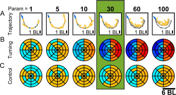
Parameter selection for moving average smoothing (A) A -s piece of an example trajectory for a fish of age dpf for a moving average window width of 1, 5, 10, 60, and 100 frames. The blue arrow indicates the direction of movement of the animal, and yellow arrows indicate the direction of total acceleration for some selected frames. Gray dots show the coordinates of the original trajectory. (B) Probability of focal animal turning to the right when second animal is in different positions in space for the corresponding values of the smoothing parameter (results are obtained from the full trajectory). (C) Same as B but for randomized control data.
Fig. S11.
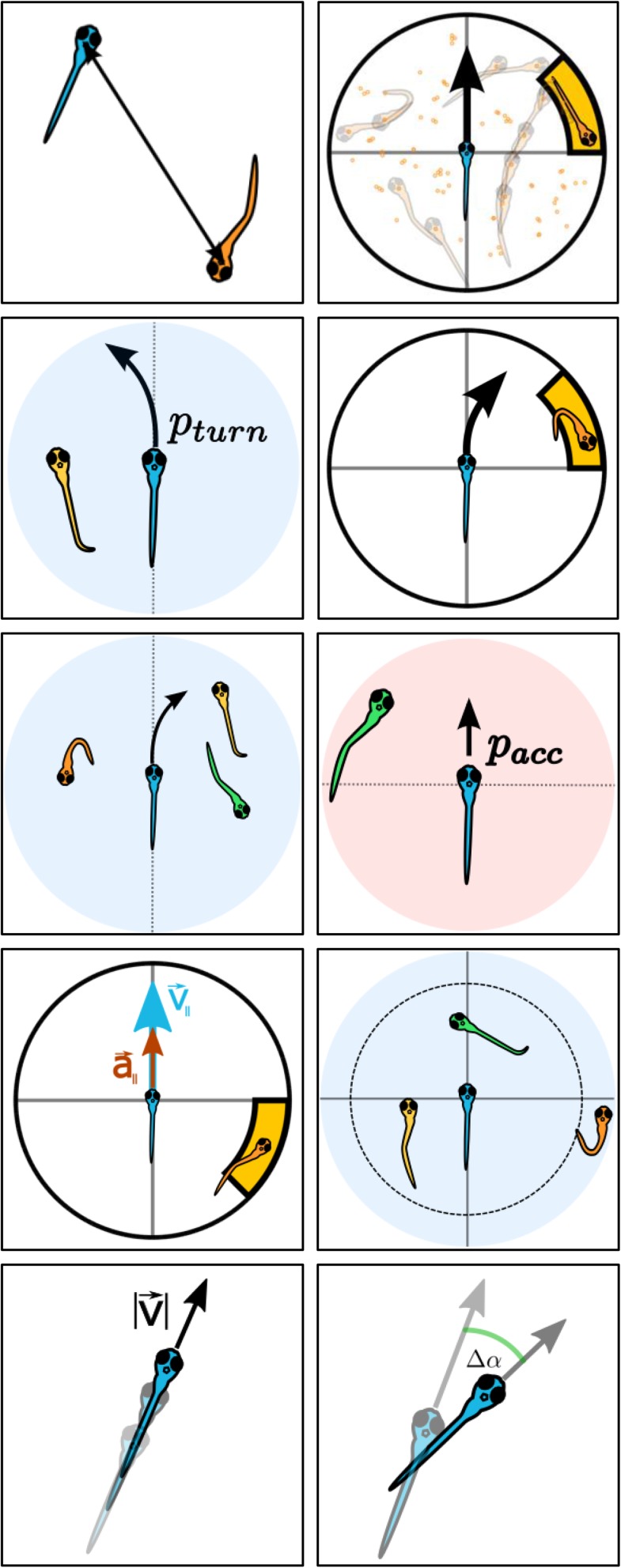
Analysis with idSocial. The following idSocial methods have been used to analyze trajectories (from top left to bottom right): Interindividual distance, relative position, turning probability (the probability of turning toward a conspecific), turning probabilities for relative positions, turning probability for groups (the probability of turning toward a specific number of conspecifics in a given configuration), acceleration probability (the probability of speeding up/slowing down depending on the position of a conspecific in front/at the back), acceleration probability for relative positions, probability of having a certain number of close neighbors, and speed and turning angle.
Control Randomized Data.
Control data are obtained by randomization of the original data. For any video of two animals with frames, we paired the position of fish in each frame , , with the position of fish in a random frame separated from by at least frames to avoid any correlations, . From the video with frames, we then get the pairs . Repeating this times with different random numbers and also for fish instead of fish , we get versions of the pairs , equivalent to having control randomized videos per experimental video.
For control randomized data in the study of acceleration of the focal, , depending on position of the second fish, we used analogous procedure to obtain the pairs .
Significance Tests.
Significance is then obtained as the probability that the control randomized data give the experimental result. Using the procedure to build control randomized data, if, for a given age, we have videos, we then obtain control videos. We illustrate in the following how to use these control videos for a significance analysis of the mean distance between two fish at a given age. For each of the experimental videos of fish pairs taken at that age (say ), we obtain a mean distance, giving values of mean distance, whose mean is . From the control videos, we extract mean distance values. We then draw random values from these and compute their mean, . This is repeated times, giving values of and we compute the value as the proportion of these with values equal to or smaller than the experimental value, .
For probability maps, we run an analogous procedure, but using repetitions for each bin of the map.
Parameter-Free Relationship Between Pairs of Configurations.
Eq. 1 implies a parameter-free relationship between any pair of asymmetric configurations ( with and with ) as
| [6] |
Calculation of the Mode.
We used kernel density estimation with an Epanechnikov kernel and a bandwidth of two BL to obtain smooth continuous distributions from which the value with maximum probability was calculated.
Agent-Based Model.
The movement of agents is simulated by fixing a set of rules for the interaction among them and with the borders of the arena. Agents move at constant speed and turn a fixed angle in the direction of a randomly chosen neighbor with probability , whereas, with probability , they choose randomly to turn left or right. The correspondence between the value and day of development is as in the data from Fig. 4F. Fig. S5 uses alternative interaction rules. For the nonsocial part of the model, we used as constant speed the mean experimental speed (Fig. S6B), the turning at a relevant experimental value (Fig. S6C), and interactions with the borders of arena mimicking experimental ones (SI Text).
SI Text
Tracking and Trajectory Smoothing
The extraction of the coordinates of each individual in each video frame was done automatically by idTracker. Those frames in which the probability of the identity assigned to an individual by idTracker was below were neglected in all following analyses of this individual.
Coordinates in idTracker are calculated as the center of mass of the set of pixels corresponding to each animal in a video frame. As such, they are subject to noise due to fluctuations in illumination and in the posture of the animals. Although noise only leads to small deviations in the x–y coordinates, it has a greater effect on the velocity and, especially, the acceleration of an animal, which are calculated from the coordinates.
Moreover, the trajectory of an animal contains information on movements belonging to different time scales, for example, quick undulating movements that fish use to propel themselves forward and slower changes of direction used to approach conspecifics or destinations within the arena.
To both account for the noise and be able to analyze different time scales, we applied a simple “moving average smoothing,” which calculates the coordinate of an individual in a frame as the mean over a fixed number of frames previous and subsequent to this frame. In our analysis, a trajectory obtained by idTracker is split into its x and y coordinates, which are then smoothed separately. The width of the smoothing window and thus the time scale was carefully chosen, applying two criteria: Firstly, we manually checked that coordinates taken from the smoothed trajectory did not deviate excessively from those taken from the original trajectory, by overlaying the resulting trajectory on top of the original video. Fig. S10A illustrates how the smoothing parameter affects the deviation from the original trajectory. Secondly, we compared results from various smoothing parameters. Fig. S10B shows maps of the probability of turning to the right depending on the relative position of the neighbor for smoothing parameters ranging from to frames (0.03 to 3 s). Although the left–right pattern in the turning maps gets more pronounced with increasing parameter values, the controls from randomization also develop a similar pattern. This similarity is due to the fact that both the probability of turning toward the center of the arena and the probability of finding the conspecific in the same direction as the center of the arena increase for individuals who are close to the border (Fig. S6D). Combining these criteria, we chose a window width of frames (corresponding to 0.9 s), a value for which the resulting patterns are clearly visible, but still not too pronounced in the randomized controls.
The velocity vector of an individual in frame is then calculated from its smoothed trajectory as the difference between its x–y coordinates in frame and frame , , and acceleration is calculated as . Using distance, relative distance, and these smoothed velocity and acceleration vectors, the toolbox idSocial (downloadable from www.idtracker.es/idsocial) gives a variety of methods to study interactions (Fig. S11).
Trajectory Filtering
In all analyses, only those frames were taken into account in which the focal animal was moving with a speed greater than 0.1 BL/s; this was done because the velocity and acceleration (and therefore also direction of movement) can only be calculated reliably from the trajectory if coordinates in adjacent frames are sufficiently apart from each other. In addition, by restricting our analyses to moving animals, we avoid ambiguous results like small interindividual distances resulting from the aggregation of motionless animals for nonsocial reasons. Those trials in which all animals were present simultaneously (i.e., their identities were not lost by idTracker due to crossings, and the probability of the identity assigned to each animal in the frame is >0.9) in less than 20% of all frames were discarded.
For some of the analyses, additional filters were applied to trajectories: The turning () and acceleration () probabilities in Fig. 3A and Figs. S2D, S3D, S4A, S7H, S8A, and S9G were calculated from frames in which the distance between individuals was smaller than six BL, corresponding to the maximum radius of the maps shown in Figs. 2B and 3B.
Turning probabilities in Fig. 4 are obtained for each focal individual only from frames in which all neighbors were farther away than 2.5 BL, to exclude effects resulting from close-range interaction between animals. The radius of 2.5 BL coincides with the range of reduced attraction determined in Fig. S6A.
For results shown in Fig. 4, only frames in which all animals were present (i.e., their positions were successfully determined by idTracker and were not lost, for example, due to crossings of various animals) were used in the analysis to guarantee that the configuration () of neighbors could be determined correctly. To reduce the effect of the border, only frames in which the focal animal was within a radius of (radius of the arena) from the center of the arena were taken into account for group sizes two and four animals, and (radius of the arena) for a group size of seven animals.
Simulation
Outline.
The movement of agents is simulated by fixing a set of rules for the interaction between various agents and interactions between the agents and the borders of a circular arena. Agents turn in the direction of a randomly chosen neighbor with a probability , whereas, with a probability , they choose randomly to turn left or right. Repulsion from the border is obtained by increasing the probability of turns toward the center when agents get close to the border of the arena and by letting them move parallel to the walls when they touch the border. In addition, simulations presented in Fig. S9 incorporate reduced attraction at close interindividual distances by decreasing the social weight within a fixed radius around each agent, and repulsion is simulated by a sharp increase in speed when an agent is approached by another from behind.
Parameters and Movement Variables.
These rules are implemented using the following parameters and variables:
-
•
External parameters follow our experimental results:
The border of the arena is defined by a circle with radius BL. The BL for each age is obtained from experiments. Because the ratio of radius and absolute BL is kept constant throughout all experiments, the BL in pixels stays approximately constant at around 50 pixels (whereas the absolute BL increases as in Fig. S3A), and so does the diameter, which is ∼ pixels. The arena is centered at x–y coordinates .
The sampling time determines with which frequency the position and orientation of each agent is updated. In our simulations, we choose s, which is half the time between frames in our experimental videos (at a frame rate of 33 fps to 34 fps).
The update time determines the frequency at which the interaction state of each agent is updated (“social” or “nonsocial”; see Simulation, Update of Interaction State). The updated state will stay the same for a period of time steps. At the beginning of each period, each agent is selected to either interact socially with one of its neighbors or not to interact with any agent. The update time is set to s, matching the frame rate of our experimental videos. Simulations with different update times between s and s do not differ strongly from results for s.
The step width by which each agent can move between adjacent time steps is taken from the mean speed obtained from experimental results (Fig. S6B). Because the experimental speed is calculated for a fixed frame rate , the step width is extrapolated according to the sampling rate of the simulation , and thus , with pixels/frame.
The turning angle by which an agent can change its orientation between two time steps is set to rad, a value that was chosen considering the distribution of experimentally obtained turning angles, which show no clear change with age (Fig. S6C). The chosen value corresponds approximately to the 83rd percentile of the distributions.
Repulsion from the borders of the arena is simulated in terms of an increase in the probability of turns away from the border/toward the center of the arena. Experimental results that we obtain by pooling data from single-animal experiments of age dpf to dpf show that animals tend to increase the probability of turning toward the center of the arena (Fig. S6D) when they are close to the borders of the arena. We approximate the probability of turning toward the center by a piecewise linear fit: In an arena of radius , the probability of an individual turning toward the center when being at a distance from the center is given by
| [S1] |
where is defined by
| [S2] |
To determine if an agent has to turn to the left or to the right to turn toward the center, the angle between the direction of movement of agent and the unit vector pointing from agent to the center of the arena is calculated from
| [S3] |
The angle lies in the range and is (in contrast to standard use) measured clockwise, i.e., is positive (negative) if the center is at the right (left) hand side of agent .
Here, is the four-quadrant inverse tangent (as calculated by the Matlab function “atan2”) defined by
| [S4] |
The probability of interacting socially with a neighbor is captured by the social weight . We perform simulations with values of taken from experimental data (Fig. 4F).
As can be seen from experimental data, the probability of an animal turning toward its conspecific depends on the distance between the two animals (Fig. S6A) and increases steadily from 0.5 (corresponding to randomly turning toward or away from the neighbor) at distance 0 until reaching a limit value at a distance of about 2.5 BL. This behavior is simulated by adjusting the social weight when a neighbor is found within the radius of reduced attraction from the focal,
| [S5] |
For the results presented in Fig. S9, is set to 2.5 BL.
In addition, animals tend to accelerate when a conspecific is approaching them from behind (Fig. S4B). For the results presented in Fig. S9, this acceleration is simulated by increasing the step width of the focal agent by the forward acceleration when a neighbor is behind and within the repulsion radius ,
| [S6] |
Acceleration is set to pixels per frame2, coinciding with the range of highest values of acceleration we observe in our data, and = = 2.5 BL. In analogy with the step width, acceleration is extrapolated to take into account the sampling rate of the simulation, resulting in .
Neither repulsion nor reduced attraction is included in the simulations presented in Agent-Based Modeling (Fig. 5) or Figs. S5 and S8.
-
•
A series of movement variables is calculated to determine the position, orientation, and interaction between agents and the repulsion from the borders of the arena:
The position of each agent within the arena at time step is defined by its x and y coordinates .
The orientation or direction of movement of each agent is given by the angle between the direction of movement of the agent and the x axis. Because the orientation determines the direction of movement, it is connected to the position by the update condition
| [S7] |
The interindividual distance between two agents and is calculated as the euclidean distance given by
| [S8] |
Social interactions between agents are calculated on the basis of the relative positions between agents, which determine if a neighbor is at the right- or left-hand side of an agent. For that purpose, the angle between the direction of movement of agent and the unit vector pointing from agent to its neighbor is calculated from
| [S9] |
The angle lies in the range and is (in contrast to standard use) measured clockwise, i.e., is positive (negative) if neighbor is at the right (left) hand side of agent .
Initial Step.
In the initial step (), the position of each agent is randomly chosen from the set of all possible combinations of x–y coordinates for which the euclidean distance from the center of the arena is smaller than ,
| [S10] |
The initial orientation at for each agent is randomly chosen from the range .
Update of Interaction State.
Every time steps, it is determined whether an agent is interacting socially or not in the following way: The real number is randomly drawn from a uniform distribution on the interval . If , agent is selected for interacting socially with one of its neighbors. Otherwise, if , its movement will be updated independently of its neighbors.
Update of Position and Orientation.
In every time step , the position and orientation of each agent is updated using the following rules, which correspond to nonsocial behavior, attractive (social) behavior, interaction between individuals at close range, repulsion, and interactions with the arena borders. The duration of the simulation corresponds to the -min duration of our experiments.
Nonsocial behavior.
If, in the present time step, an agent has been selected for nonsocial behavior, the change of direction of agent is chosen randomly as either left () or right (), and the agent turns to the selected direction with the turning angle ,
| [S11] |
Finally, the position of agent is updated using Eq. S7.
Social behavior.
For agents that have been selected for social interactions, a neighbor is chosen randomly from the set of all available neighbors, with . Social interaction is then modeled as a turn toward the neighbor , and the orientation is updated to
| [S12] |
where is given by
| [S13] |
The preliminary position of each agent is updated as in Eq. S7, but can still be changed due to interaction with close neighbors or repulsion with either a neighbor or the arena borders.
Interaction between close individuals.
For results presented in Fig. S9, the probability of turning toward the neighbor is reduced for agents that have previously been selected for social interactions and whose randomly chosen neighbor is closer than .
At each time step , for each agent , the distance (Eq. S8) to all of its neighbors is calculated. If the selected neighbor is closer than , , the probability of turning toward the neighbor is reduced, and the position update is repeated in the following way:
-
i)
The real number is randomly drawn from a uniform distribution on the interval . If , agent is selected for interacting socially with its closest neighbor. Otherwise, if , its movement will be updated independently of its neighbors.
-
ii)
Social interaction is modeled as a turn toward the selected neighbor in the same way as described in Social behavior. If the agent is not interacting socially, its position is updated as described in Nonsocial behavior.
Repulsion between close agents.
If a neighbor can be found within the repulsion radius () and behind the focal animal (), the focal animal will move with the increased step width while maintaining the previously determined turning angle , and the position update is repeated by
| [S14] |
Nonsocial behavior close to the border.
Those agents that are positioned at a distance greater than from the center of the arena and that have not been selected for social behavior are determined, and their position and orientation is reupdated using the following rule: The orientation of each of the agents with regard to the center of the arena is determined by calculating the angle (Eq. S3). To determine the direction of turn for the next update, the real number is randomly drawn from a uniform distribution on the interval . If (), agent is updated using a turn toward (away from) the center,
| [S15] |
and the position is then updated following Eq. S7.
Repulsion from border.
In the rare case that, despite the increasing bias of turning toward the arena center, the distance between the agent and the center of the arena would be greater than after the update,
| [S16] |
the update step is repeated, and the direction of movement of this individual is updated to be parallel to the border of the arena instead. This rule is applied both to agents selected for social behavior and to agents selected for nonsocial behavior. To simulate this movement along the walls, the x–y coordinates are first converted into polar coordinates, with the origin given by the center of the arena and angles measured with regard to the positive x axis. The angular coordinate is calculated by
| [S17] |
A movement along the arena border with a step width that starts and ends at a distance from the center equals a change in of
| [S18] |
(Note that is a real number only if , which is true for the parameter values chosen in our simulations, in particular for all values of and .) The angular coordinate is then updated to
| [S19] |
Here, is used to guarantee that the agent maintains the same orientation with respect to the center of the arena that it had before the update, i.e., that it will move counterclockwise if, before, the center was at its right-hand side, and clockwise otherwise. Finally, the position of the agent is calculated from the new angular coordinate as
| [S20] |
The updated orientation is calculated using the vector pointing from the position at time step to the position at time step ,
| [S21] |
which yields
| [S22] |
Analysis.
For the analyses presented in Fig. 5 and Figs. S5, S8, and S9, the same methods were used as for the corresponding analysis of experimental data, with the exception that, for simulations without repulsion and distance-dependent attraction, neighbors closer than BL were not filtered out. No smoothing was applied to the trajectories obtained from simulations. Because the update rate is twice as high in the simulations as the sampling rate (i.e., the frame rate) of the experiments, simulated trajectories are downsampled by only taking every second time step before starting the analysis.
Acknowledgments
We thank Mattia Bergomi, Iain Couzin, Andres Laan, Alfonso Perez-Escudero, and Michael Orger for discussions; Isidro Dompablo (CSIC) and Ana Catarina Certal (Fundação Champalimaud) for animal care; and Paulo Carriço (Fundação Champalimaud) for technical assistance with setups. This work was supported by Spanish Plan Nacional Ministerio de Economia y Competitividad Grants BFU2012-33448 and BFU2013-49512-EXP (to G.G.d.P.), Fundação para a Ciência e Tecnologia PTDC/NEU-SCC/0948/2014 (to G.G.d.P.), and Fundação Champalimaud (to G.G.d.P.). The funders had no role in study design, data collection and analysis, decision to publish, or preparation of the manuscript.
Footnotes
The authors declare no conflict of interest.
This article is a PNAS Direct Submission.
Data deposition: Data were deposited at www.idtracker.es/idsocial.
This article contains supporting information online at www.pnas.org/lookup/suppl/doi:10.1073/pnas.1616926114/-/DCSupplemental.
References
- 1.Krause J, et al. Fish shoal composition: Mechanisms and constraints. Proc R Soc London Ser B. 2000;267(1456):2011–2017. doi: 10.1098/rspb.2000.1243. [DOI] [PMC free article] [PubMed] [Google Scholar]
- 2.Croft DP, et al. Mechanisms underlying shoal composition in the Trinidadian guppy, Poecilia reticulata. Oikos. 2003;100(3):429–438. [Google Scholar]
- 3.Ballerini M, et al. Interaction ruling animal collective behavior depends on topological rather than metric distance: Evidence from a field study. Proc Natl Acad Sci USA. 2008;105(4):1232–1237. doi: 10.1073/pnas.0711437105. [DOI] [PMC free article] [PubMed] [Google Scholar]
- 4.Nagy M, Akos Z, Biro D, Vicsek T. Hierarchical group dynamics in pigeon flocks. Nature. 2010;464(7290):890–893. doi: 10.1038/nature08891. [DOI] [PubMed] [Google Scholar]
- 5.Attanasi A, et al. Collective behaviour without collective order in wild swarms of midges. PLoS Comput Biol. 2014;10(7):e1003697. doi: 10.1371/journal.pcbi.1003697. [DOI] [PMC free article] [PubMed] [Google Scholar]
- 6.Strandburg-Peshkin A, Farine DR, Couzin ID, Crofoot MC. Shared decision-making drives collective movement in wild baboons. Science. 2015;348(6241):1358–1361. doi: 10.1126/science.aaa5099. [DOI] [PMC free article] [PubMed] [Google Scholar]
- 7.Ward AJW, Sumpter DJT, Couzin ID, Hart PJB, Krause J. Quorum decision-making facilitates information transfer in fish shoals. Proc Natl Acad Sci USA. 2008;105(19):6948–6953. doi: 10.1073/pnas.0710344105. [DOI] [PMC free article] [PubMed] [Google Scholar]
- 8.Sumpter DJT. Collective Animal Behavior. Princeton Univ Press; Princeton: 2010. [Google Scholar]
- 9.Katz Y, Tunstrøm K, Ioannou CC, Huepe C, Couzin ID. Inferring the structure and dynamics of interactions in schooling fish. Proc Natl Acad Sci USA. 2011;108(46):18720–18725. doi: 10.1073/pnas.1107583108. [DOI] [PMC free article] [PubMed] [Google Scholar]
- 10.Herbert-Read JE, et al. Inferring the rules of interaction of shoaling fish. Proc Natl Acad Sci USA. 2011;108(46):18726–18731. doi: 10.1073/pnas.1109355108. [DOI] [PMC free article] [PubMed] [Google Scholar]
- 11.Perna A, et al. Individual rules for trail pattern formation in Argentine ants (Linepithema humile) PLoS Comput Biol. 2012;8(7):e1002592. doi: 10.1371/journal.pcbi.1002592. [DOI] [PMC free article] [PubMed] [Google Scholar]
- 12.Miller N, Gerlai R. Quantification of shoaling behaviour in zebrafish (Danio rerio) Behav Brain Res. 2007;184(2):157–166. doi: 10.1016/j.bbr.2007.07.007. [DOI] [PubMed] [Google Scholar]
- 13.Romenskyy M, Herbert-Read JE, Ward AJW, Sumpter DJT. 2015. The statistical mechanics of schooling fish captures their interactions. arXiv:1508.07708.
- 14.Arganda S, Pérez-Escudero A, de Polavieja GG. A common rule for decision making in animal collectives across species. Proc Natl Acad Sci USA. 2012;109(50):20508–20513. doi: 10.1073/pnas.1210664109. [DOI] [PMC free article] [PubMed] [Google Scholar]
- 15.Hamilton W. Geometry for the selfish herd. J Theor Biol. 1971;31(2):295–311. doi: 10.1016/0022-5193(71)90189-5. [DOI] [PubMed] [Google Scholar]
- 16.Vicsek T, Czirok A, Ben-Jakob E, Cohen I, Shochet O. Novel type of phase transition in a system of self-driven particles. Phys Rev Lett. 1995;75(6):1226–1229. doi: 10.1103/PhysRevLett.75.1226. [DOI] [PubMed] [Google Scholar]
- 17.Inada Y, Kawachi K. Order and flexibility in the motion of fish schools. J Theor Biol. 2002;214(3):371–387. doi: 10.1006/jtbi.2001.2449. [DOI] [PubMed] [Google Scholar]
- 18.Couzin ID, Krause J, James R, Ruxton GD, Franks NR. Collective memory and spatial sorting in animal groups. J Theor Biol. 2002;218(1):1–11. doi: 10.1006/jtbi.2002.3065. [DOI] [PubMed] [Google Scholar]
- 19.Couzin ID, Krause J, Franks NR, Levin SA. Effective leadership and decision-making in animal groups on the move. Nature. 2005;433(7025):513–516. doi: 10.1038/nature03236. [DOI] [PubMed] [Google Scholar]
- 20.Lukeman R, Li YX, Edelstein-Keshet L. Inferring individual rules from collective behavior. Proc Natl Acad Sci USA. 2010;107(28):12576–12580. doi: 10.1073/pnas.1001763107. [DOI] [PMC free article] [PubMed] [Google Scholar]
- 21.Pérez-Escudero A, de Polavieja GG. Collective animal behavior from Bayesian estimation and probability matching. PLoS Comput Biol. 2011;7(11):e1002282. doi: 10.1371/journal.pcbi.1002282. [DOI] [PMC free article] [PubMed] [Google Scholar]
- 22.Ward AJW, Herbert-Read JE, Sumpter DJT, Krause J. Fast and accurate decisions through collective vigilance in fish shoals. Proc Natl Acad Sci USA. 2011;108(6):2312–2315. doi: 10.1073/pnas.1007102108. [DOI] [PMC free article] [PubMed] [Google Scholar]
- 23.Bode NWF, Franks DW, Wood AJ. Limited interactions in flocks: Relating model simulations to empirical data. J R Soc Interface. 2011;8(55):301–304. doi: 10.1098/rsif.2010.0397. [DOI] [PMC free article] [PubMed] [Google Scholar]
- 24.Ward AJW, Krause J, Sumpter DJT. Quorum decision-making in foraging fish shoals. PLoS One. 2012;7(3):e32411. doi: 10.1371/journal.pone.0032411. [DOI] [PMC free article] [PubMed] [Google Scholar]
- 25.Lopez U, Gautrais J, Couzin ID, Theraulaz G. From behavioural analyses to models of collective motion in fish schools. Interface Focus. 2012;2(6):693–707. doi: 10.1098/rsfs.2012.0033. [DOI] [PMC free article] [PubMed] [Google Scholar]
- 26.Vicsek T, Zafeiris A. Collective motion. Phys Rep. 2012;517(3-4):71–140. [Google Scholar]
- 27.Weitz S, et al. Modeling collective animal behavior with a cognitive perspective: A methodological framework. PLoS One. 2012;7(6):e38588. doi: 10.1371/journal.pone.0038588. [DOI] [PMC free article] [PubMed] [Google Scholar]
- 28.Pritchard VL, Lawrence J, Butlin RK, Krause J. Shoal choice in zebrafish, Danio rerio: The influence of shoal size and activity. Anim Behav. 2001;62(6):1085–1088. [Google Scholar]
- 29.Engeszer RE, Ryan MJ, Parichy DM. Learned social preference in zebrafish. Curr Biol. 2004;14:881–884. doi: 10.1016/j.cub.2004.04.042. [DOI] [PubMed] [Google Scholar]
- 30.Engeszer RE, Patterson LB, Rao AA, Parichy DM. Zebrafish in the wild: A review of natural history and new notes from the field. Zebrafish. 2007;4(1):21–40. doi: 10.1089/zeb.2006.9997. [DOI] [PubMed] [Google Scholar]
- 31.Buske C, Gerlai R. Maturation of shoaling behavior is accompanied by changes in the dopaminergic and serotoninergic systems in zebrafish. Dev Psychol. 2012;54(1):28–35. doi: 10.1002/dev.20571. [DOI] [PMC free article] [PubMed] [Google Scholar]
- 32.Hinz FI, Aizenberg M, Tushev G, Schuman EM. Protein synthesis-dependent associative long-term memory in larval zebrafish. J Neurosci. 2013;33(39):15382–15387. doi: 10.1523/JNEUROSCI.0560-13.2013. [DOI] [PMC free article] [PubMed] [Google Scholar]
- 33.Dreosti E, Lopes G, Kampff AR, Wilson SW. Development of social behavior in young zebrafish. Front Neural Circuits. 2015;9:39. doi: 10.3389/fncir.2015.00039. [DOI] [PMC free article] [PubMed] [Google Scholar]
- 34.Pérez-Escudero A, Vicente-Page J, Hinz RC, Arganda S, de Polavieja GG. idTracker: Tracking individuals in a group by automatic identification of unmarked animals. Nat Methods. 2014;11(7):743–748. doi: 10.1038/nmeth.2994. [DOI] [PubMed] [Google Scholar]
- 35.Krause J, Tegeder RW. The mechanism of aggregation behaviour in fish shoals: Individuals minimize approach time to neighbours. Anim Behav. 1994;48(2):353–359. [Google Scholar]
- 36.Viscido SV, Miller M, Wethey DS. The dilemma of the selfish herd: The search for a realistic movement rule. J Theor Biol. 2002;217(2):183–194. doi: 10.1006/jtbi.2002.3025. [DOI] [PubMed] [Google Scholar]
- 37.Viscido S, Parrish JK, Grünbaum D. Individual behavior and emergent properties of fish schools: A comparison of observation and theory. Mar Ecol Prog Ser. 2004;273:239–249. [Google Scholar]
- 38.Viscido SV, Parrish JK, Grünbaum D. The effect of population size and number of influential neighbors on the emergent properties of fish schools. Ecol Modell. 2005;183(2-3):347–363. [Google Scholar]
- 39.Reluga TC, Viscido S. Simulated evolution of selfish herd behavior. J Theor Biol. 2005;234(2):213–225. doi: 10.1016/j.jtbi.2004.11.035. [DOI] [PubMed] [Google Scholar]
- 40.Kimbell HS, Morrell LJ. ‘Selfish herds’ of guppies follow complex movement rules, but not when information is limited. Proc Biol Sci. 2015;282(1816):20151558. doi: 10.1098/rspb.2015.1558. [DOI] [PMC free article] [PubMed] [Google Scholar]
- 41.Orger MB, Kampff AR, Severi KE, Bollmann JH, Engert F. Control of visually guided behavior by distinct populations of spinal projection neurons. Nat Neurosci. 2008;11(3):327–333. doi: 10.1038/nn2048. [DOI] [PMC free article] [PubMed] [Google Scholar]
- 42.Ahrens MB, et al. Brain-wide neuronal dynamics during motor adaptation in zebrafish. Nature. 2012;485(7399):471–477. doi: 10.1038/nature11057. [DOI] [PMC free article] [PubMed] [Google Scholar]
- 43.Severi KE, et al. Neural control and modulation of swimming speed in the larval zebrafish. Neuron. 2014;83(3):692–707. doi: 10.1016/j.neuron.2014.06.032. [DOI] [PMC free article] [PubMed] [Google Scholar]


