Early Detection of Heart Failure Using Electronic Health Records: Practical Implications for Time before Diagnosis, Data Diversity, Data Quantity and Data Density

Abstract

Background

Using electronic health records (EHR) data to predict events and onset of diseases is increasingly common. Relatively little is known, though, about the tradeoffs between data requirements and model utility.

Methods and Results

We examined the performance of machine learning models trained to detect pre-diagnostic heart failure (HF) in primary care patients using longitudinal EHR data. Model performance was assessed in relation to data requirements defined by: the prediction window length (time before clinical diagnosis), the observation window length (duration of observation prior to prediction window), the number of different data domains (data diversity), the number of patient records in the training data set (data quantity) and the density of patient encounters (data density). A total of 1,684 incident HF cases and 13,525 gender, age-category, and clinic matched controls were used for modeling. Model performance improved as: 1) the prediction window length decreases, especially when less than 2 years; 2) the observation window length increases but then levels off after 2 years; 3) the training data set size increases but then levels off after 4000 patients; 4) more diverse data types are used, but, in order, the combination of diagnosis, medication order, and hospitalization data were most important; and 5) data were confined to patients who had 10 or more phone or face-to-face encounters in two years.

Conclusions

These empirical findings suggest possible guidelines for the minimum amount and type of data needed to train effective disease onset predictive models using longitudinal EHR data.

Introduction

For those 40 years of age the lifetime risk of developing heart failure (HF) is 20%.[1] Diagnosis is associated with a high level of disability, health care costs and mortality (i.e., ~50% within 5 years of diagnosis)[2], [3]. Earlier detection of HF opens the possibility to test means to preserve cardiac function and change the natural history of disease onset. The rapid growth of health systems with electronic health records (EHRs) in the past 15 years opens new opportunities to implement early detection surveillance. However, the success that any health system will have in detecting HF early with predictive methods will depend on patient level data diversity, quantity and density.

Information that can be gained on populations of patients from longitudinal EHR data can be used to individualize care for a given patient. Access to these data in combination with the rapid evolution of modern machine learning and data mining techniques offer a potentially promising means to accelerate discoveries that can be readily translated to clinical practice.

Rapid growth in the application of machine learning methods to EHR for predicting future patient outcomes is fostering a deeper understanding of best practices and the tradeoffs between model performance and patient coverage (i.e., the percent of potentially eligible patients for which risk assessment can be completed)[4]–[7]. Model utility for a given system will strongly depend on the length of the prediction window, the length of the observation window, and the diversity, quantity and density of the available data. A longer prediction window (i.e., the duration of time before diagnosis that disease is detected) would likely increase the potential for successful prevention, but accuracy may decrease. Model performance will improve, to some degree, as the observation window (i.e., duration of time before the prediction window from which data are used) increases. But, patient coverage decreases (i.e., more patients will be excluded from risk assessment) because of the more stringent data requirement. The diversity (Table 1) of available data may also influence how well a model performs. Performance will likely improve as more different data domains are used. However, as the number of required data domains increases, it will become more challenging for health systems to make use of developed predictive models. Moreover, some data domains (e.g., diagnostic codes) may be more useful than others and there may be a diminishing return when the threshold of one or more qualifying combinations is reached. Finally, performance will likely depend on the overall amount (i.e., the number of case and control patients) and density of the available data.

Table 1.

EHR data types, examples, number of unique variables and number of grouped variables

Data Type	Examples	Number of Unique Variables	Number of Grouped Variables
Diagnoses*	ICD-9 codes (from outpatient visits and problem lists treated separately).	12616	189
Medications†	Beta blockers, loop diuretics, etc.	3952	631
Labs‡	Cholesterol, glucose, eGFR, etc.	2336	-
Hospitalization§	ICD-9 codes associated with admission	7071	189
Demographics and Health Behaviors	Age, Sex, Race/Ethnicity, smoking, alcohol use	5	-
Cardiovascular Imaging Orders#	2D echo, trans esophageal echo, stress echo, etc.	18	-
Vitals‡	Pulse, systolic blood pressure, diastolic blood pressure, height, weight, temperature	6	-
Framingham HF Signs and Symptoms	Positive and negative mentions of acute pulmonary edema, ankle edema, dyspnea on ordinary exertion, paroxysmal nocturnal dyspnea, etc.	28	-

^*ICD-9 codes from outpatient visits and problem lists are treated separately.

^†Normalized drug names, ignoring the dosing information, were used.

^‡The labs and vitals data types contain information about the test order and the numerical result of the test.

^§Primary and secondary ICD-9 codes associated with the hospital admission were used.

^#The imaging order type, associated ICD-9 codes, and any LVEF values were used.

Relatively little is known about the tradeoffs among these factors. To this end, we used data from a large health system to examine how well machine learning tools perform in relation to the prediction window length, observation window length, and the diversity, quantity and density of the available EHR data.

Methods

Study Design, Population, Setting, Source of Data

For this study, a nested case-control design was used on a large patient population from a health system that provided access to longitudinal EHR data. The source data were from the Geisinger Clinic which is a multispecialty group practice with a large primary care practice. All cases and controls were primary care patients. Geisinger includes 41 outpatient clinics in central and northeastern Pennsylvania. EpicCare EHR[8] was installed at Geisinger before 2001. The study was approved by an institutional review committee and the subjects gave informed consent.

Definition and Selection of Cases and Controls

Criteria for incident onset of HF were adopted from Gurwitz [9] and defined in detail elsewhere [10], [11], but relied on qualifying ICD-9 codes for HF with a minimum of three clinical encounters occurring within 12 months of each other. The date of diagnosis was assigned to the earliest of the three dates. Finally, incident cases had to have at least 18 months before the first occurrence of a HF ICD-9 code diagnosis without an indication that HF had been previously diagnosed or treated. Analysis was limited to patients who were 50 to 84 years of age at the time of HF diagnosis. Applying these criteria, a total of 1,684 incident HF cases were identified between 2003 and 2010, where the average primary care patient census was approximately 240,000, of which 28% were between 50 and 84 years of age.

Up to 10 eligible primary care clinic-, sex-, and age-matched (in 5-year age intervals) controls were selected for each incident HF case for a total of 13,525 control patients. Primary care patients were eligible as controls if they had no HF diagnosis before the date: one year post-HF diagnosis of the matched case. Control subjects were required to have their first office encounter within one year of the incident HF patient’s first office visit and have ≥1 office encounters 30 days before or any time after the case’s HF diagnosis date to ensure similar duration of observations among cases and controls. Nine or ten controls were identified for 49% of the cases. Only 1.5% of the cases had just 1 or 2 controls.

Structured Data Extraction from Longitudinal EHR Patient Data

EHR encounter data were extracted for all cases and controls from each of the eight data type domains (Table 1). Encounters included outpatient face-to-face and phone visits and inpatient visits. As shown in Table 1, the number of unique variables in each data type substantially varied.

For the diagnoses data type, ICD-9 codes from outpatient visits and problem lists are treated separately. This means that the same ICD-9 code associated with the different events were treated as separate variables. For the medications data type, normalized drug names (i.e. combining all branded names and the generic name for a medication) were used. Dosing information was not used. For the hospitalization data type the primary and secondary ICD-9 codes associated with the hospital admission were used[12]. The labs and vital signs data types contain information not only about the test order but also the numerical results of the test. From the cardiovascular imaging order data type only information about the imaging order type (2D echo, stress echo, etc.), associated ICD-9 codes, and any LVEF values were used. No other test results of the imaging orders were available.

For the diagnoses, hospitalizations and medication data types, different levels of representations were explored. For the diagnoses and hospitalizations data types, the ungrouped representation was the ICD-9 disease code (e.g., 401.0, 492.0, 584.90, etc.) while the grouped representation was the hierarchical condition categories (HCC) from the Centers for Medicare & Medicaid Services (CMS): e.g., hypertension, chronic obstructive pulmonary disease (COPD), renal failure, etc.[13] For the medications data type, the ungrouped representation was the normalized drug name (e.g., Hydrochlorothiazide, Atenolol, Lisinopril, Furosemide, etc.) while the grouped representation was the pharmacy subclass (e.g., thiazide diuretics, beta-blockers, ACE inhibitors, loop diuretics, etc.). Grouping reduces the number of available features and creates features that are less sparse. As shown in Table 1, the number of unique features drops from 12616 to 189 for the diagnoses data type, from 7071 to 189 for the hospitalizations data type and from 3952 to 631 for the medications data type.

Feature Construction from Longitudinal EHR Patient Data

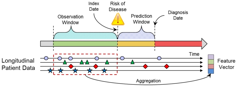
A feature vector representation for each patient was generated based on the patient’s extracted EHR data. The EHR data were represented as a temporal sequence of events (e.g. a patient can have multiple diagnoses of hypertension on different dates) in the observation window. Events of the same feature type (e.g., anti-hypertensive medication) within the observation window were represented by one or more relevant summary statistics. The summary functions can include simple feature values like Booleans, counts, means and complex feature values that can take into account temporal information (e.g., trend and temporal variation). In this study, basic aggregation functions were applied and included Booleans for categorical variables and means for numeric variables as a method to deal with irregular sampling that occurs because of variation in how patients use care. For missing aggregated values, a simple imputation approach was used. For categorical variables, the value was set to 0. For numerical variables, a single value (mean) imputation method was used. Figure 1 illustrates the relationship among the prediction window, observation window, index date and diagnosis date for cases and matching controls. The diagnosis date is the date of the clinical diagnosis for cases and the equivalent date for matched controls. The prediction window is the length of time before the diagnosis date. The index date marks the beginning of the prediction window and is the date where the risk prediction is made. The observation window specifies a period of time prior to the index date where patient data are observed. Only data in the observation window are used to represent the patient. Figure 1 also illustrates how a patient feature vector is generated by applying appropriate aggregation functions on the longitudinal EHR patient data from the observation window to combine multiple observations of the same type from different encounters in the window into a single variable.

Figure 1.

Relation of prediction window, observation window for use of data and the index and diagnosis dates for cases and the same relative times for controls.

Predictive Modeling

An initial set of experiments was performed comparing several different data driven machine learning classification approaches to select the ones to use in this study. The different classifiers compared were: random forest [14], support vector machine, k nearest neighbor, decision tree, logistic regression, and L1-regularized logistic regression. The L1-regularized logistic regression and random forest models were selected for superior predictive performance, computational efficiency, and because they represent very different modeling approaches that would be interesting to compare.

In this study, the information gain measure was used to select the top 200 most discriminating features from the original 3400+ features [15]. Interactions between the variables were not considered. Next L1-regularized logistic regression and random forest models were trained and evaluated. Unconditional logistic regression models with adjustment for continuous age were used to account for residual confounding. Internal cross validation was used to determine the model hyper-parameters: the number of features in the logistic regression model and number of trees in the random forest model.

A sequence of experiments was completed to measure how well data driven machine learning predictive modeling performs in relation to the prediction window length, the observation window length, and the diversity, quantity and density of the available EHR data. Models were trained and evaluated as detailed below. Fixed prediction window (1 year) and observation window (2 years) were used, except where specified where these parameters were evaluated.

• Data Diversity: Eight different data types (Table 1) were individually assessed on model performance. For the diagnoses and hospitalizations data types, different levels of representations of the ICD-9 codes were explored. For the medications data type, different levels of representation of the medications were explored. Models were also trained and evaluated using data type combinations starting with demographics/health behaviors and then adding vitals, diagnoses, medications, labs, Framingham Heart HF signs and symptoms [5], [6], hospitalizations and imaging to characterize the impact of using more data types.

• Prediction Window Length: Varied from 30 days to 5 years.

• Observation Window Length: Varied from 60 days to 5 years.

• Data Quantity: Varied in the amount of randomly selected training data that ranged from 114 to 11400 patients and evaluated on a held out testing data set while keeping the case/control ratio constant.

• Data Density: Different amounts of data were selected based on the number of encounters in the observation window.

10-fold cross validation was used in all modeling iterations (which includes both the initial feature selection step and the classifier training step) to make efficient use of the available data and to obtain an estimate of how well the model can generalize to an independent data set. Prediction performance was assessed by the mean and standard error of the area under the ROC curve (AUC) metrics computed over the cross validation folds. The experiments used a combination of software tools developed in house and based on open source packages for Python[16] and R[17].

Results

Performance as a Function of the Data Diversity

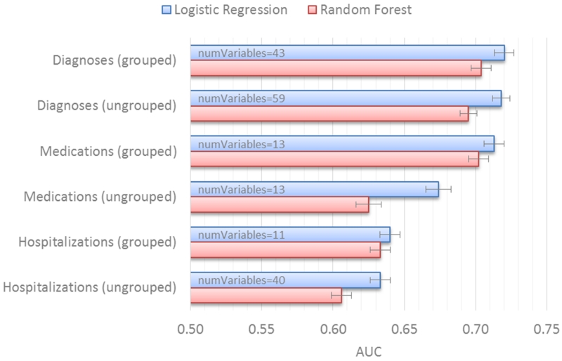
Figure 2 shows the prediction performance for ungrouped versus grouped representations for the diagnoses, medications and hospitalizations data types when used individually (i.e., unique formats represented in the EHR). The approach to grouping, based on HCC, relies on a knowledge driven hierarchy and was used to eliminate correlated and redundant features as a means to enhance model performance by allowing other useful features to be selected by the model. For each of these three data types (Figure 2), the grouped representation performs as well as or better than the non-grouped representation. The logistic regression models using the grouped representation were also less complex than those using the non-grouped representations as measured by the number of model features. For ICD-9 codes, the difference in the number of selected variables was 43 versus 59 for the diagnoses type and 11 versus 40 for the hospitalizations type. For the medications data type, both representations have 13 selected variables, but the grouped representation has significantly better performance: AUC 0.708 versus 0.674, p < 0.01. Table 2 lists some examples of the top selected grouped features for the diagnoses, hospitalization and medications data types. For the rest of the experiments in this study we used the grouped representations for the diagnoses, hospitalizations, and medications data types.

Figure 2.

Prediction performance for ungrouped versus grouped representations for the diagnoses, medications and hospitalizations data types.

Table 2.

Example feature groups for the diagnoses, hospitalizations and medications data types.

Diagnoses	Hospitalizations	Medications
Blood Disorders	Cardiac Disorders	ACE Inhibitors
Cardiac Disorders	ENT Disorders	Alpha-Beta Blockers
Cerebrovascular Disease	Eye Diseases	Angiotensin II Receptor Antagonists
Coronary Atherosclerosis	Gastrointestinal Disorders	Antiarrhythmics Type III
Diabetes	Injuries	Antidiabetic Combinations
Gastrointestinal Disorders	Lung Disease	Beta Blockers Cardio-Selective
Heart Arrhythmias	Musculoskeletal Disorders	Cardiac Glycosides
Heart Infection	Skin Diseases	Coumarin Anticoagulants
Kidney Disorders	Symptom Disorders	Insulin
Lung Disease		Loop Diuretics
Metabolic Diseases		Nitrates
Musculoskeletal Disorders		Platelet Aggregation Inhibitors
Neoplasm		Sympathomimetics
Neurological Diseases
Polyneuropathy
Vascular Disease

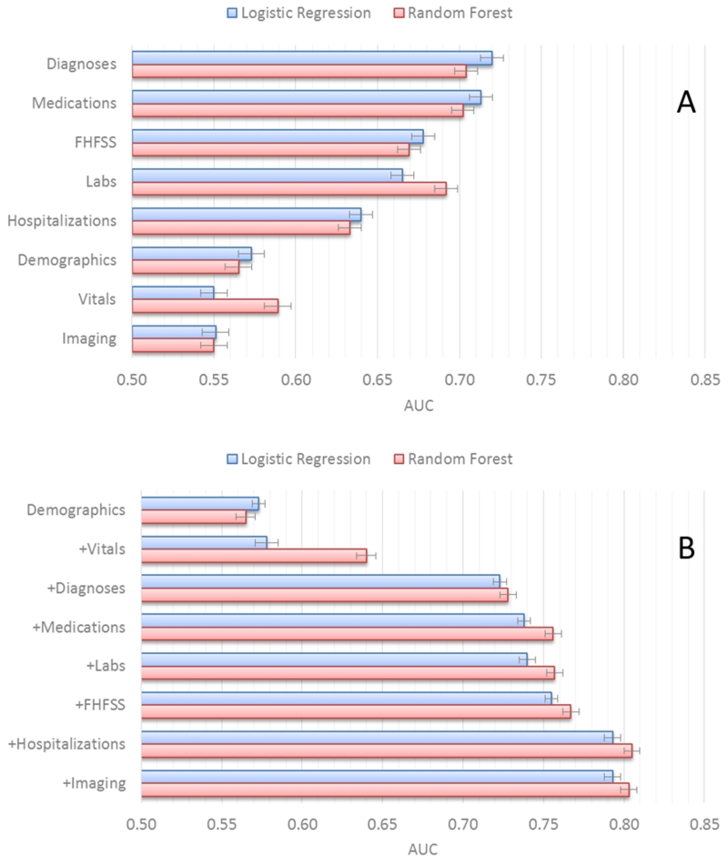
Individually, diagnosis and medication order data types performed best (Figure 3A), followed by lab test and hospitalization data types. Demographics/health behaviors, imaging test orders, and vitals data types perform the worst on their own.

Figure 3.

Prediction performance for (A) individual and (B) combined data types.

Figure 3B shows prediction performance as data types are used in combination starting with demographics/health behaviors and adding vitals, diagnoses, medications, labs, hospitalizations and imaging. The combination sequence is based on our assessment of the availability of each of the data types from most to least common. Use of only the demographics/health behaviors and vitals data types did not yield models that perform well. Adding in the diagnoses data type results in a large increase in model performance (AUC 0.733 versus 0.581, p < 0.00001). The addition of the medications data type results in a small but significant performance improvement (AUC 0.752 versus 0.733, p < 0.05). Adding the labs data type did not significantly improve model performance. In contrast, addition of the hospitalization data type significantly improved performance (AUC 0.791 versus 0.756, p < 0.001). Finally, the addition of the imaging data types did not significantly improve performance.

Supplemental Table S1 lists the selected variables and related statistics for the L1-regularized logistic regression models trained on 90% of the data from one of the cross validation folds using all the data types. The variables selected for the other cross validation folds were very similar. Hospitalization, diagnosis, medication, and lab features dominated. A few of the Framingham HF signs/symptoms and imaging variables were also selected. None of the demographic/health behaviors or vital features was selected.

Supplemental Table S2 shows the top variables selected in the random forest model based on the variable importance score [14]. A random forest classifier was built, measuring how much the classification output changes as each input feature variable is randomly changed. Important input features are expected to substantially improve classification output value, while changes to an unimportant input feature will not affect the output much. The variable importance scores from the random forest classifier trained on each of the ten cross validation folds were averaged and represented as composite scores to then rank the features. The random forest classifier uses many more features from all data types except imaging than the logistic regression classifier. For the rest of the experiments in this study we used all eight of the data types. Descriptions of all the variables appearing in Supplemental Tables S2 and S3 are listed in Supplemental Table S3.

Performance as a Function of Prediction Window Length

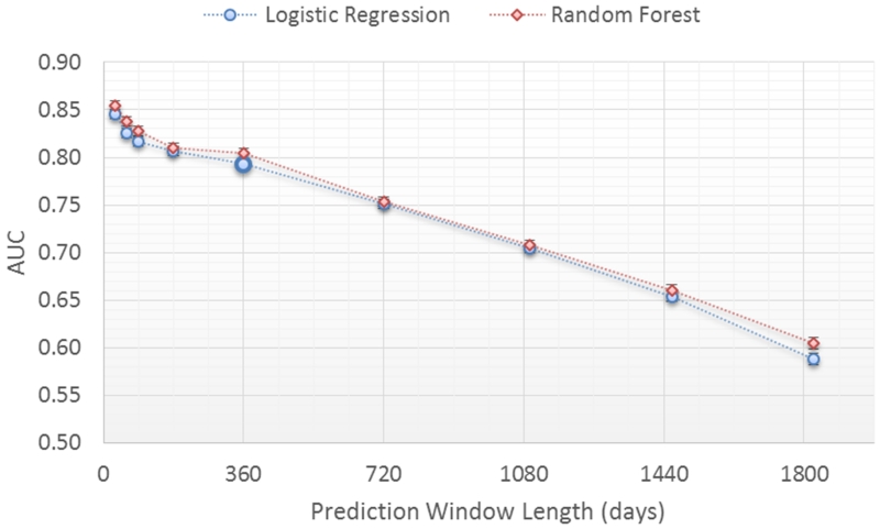
The impact on model performance was evaluated for a window length of 30 days to 5 years (Figure 4) with a fixed two year observation window. The prediction window length specifies the amount of time before the true clinical HF diagnosis that the prediction is performed (Figure 1). As expected, performance for both classifiers declines in relation to increasing prediction window length (i.e., the time before the actual clinical diagnosis). Prediction performance is at or above 0.80 AUC for prediction windows less than or equal to 1 year. Performance is at 0.74 AUC for a 2 year prediction window. Performance then declines rapidly for prediction window lengths longer than 2 years.

Figure 4.

Prediction performance for different prediction window lengths.

Performance as a Function of Observation Window Length

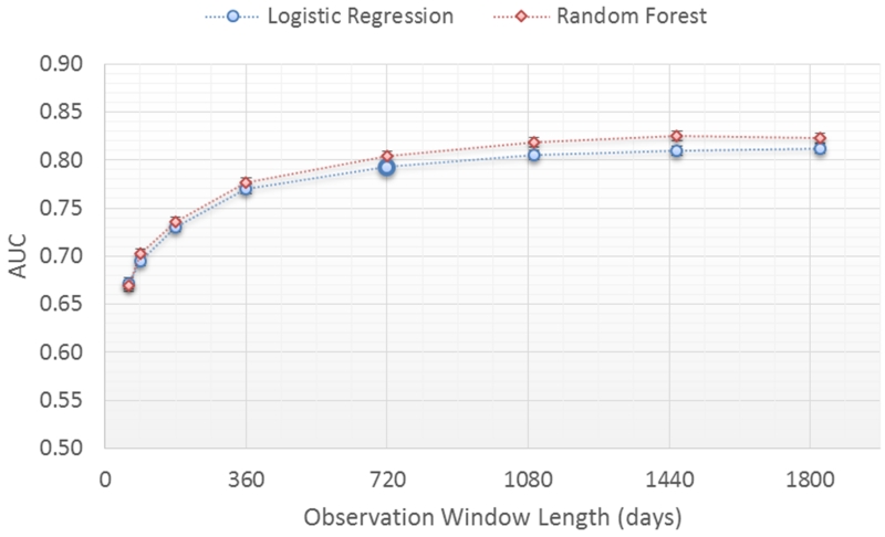
The impact of model performance was evaluated in relation to the observation window length ranging from 60 days to 5 years (Figure 5) with a fixed prediction window length of 1 year. The observation window length specifies the length of time in the patient record from which data are extracted to represent the patient (Figure 1). The longer the observation window the more data points from the patient record are used except, of course, where patient time under observation is shorter than the observation window. For both classifiers, prediction performance improves steadily as the observation window length increases up until 2 years where the performance reaches 0.79 AUC. Longer observation windows (3, 4 and 5 years) had minimal impact on model performance (up to 0.80 AUC).

Figure 5.

Prediction performance for different observation window lengths.

Performance as a Function of the Training Set Size

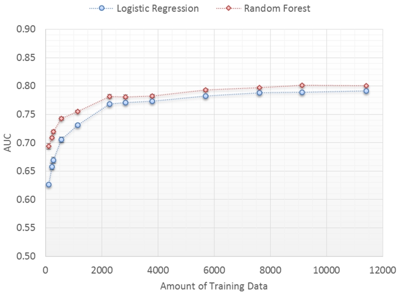
The original data set is randomly split into 25% (3802 patients) for testing and 75% (11407 patients) for training. The training set was randomly sampled (without replacement) and varied from 114 to 11407 patients in size to train the classifiers and then used to score the patients in the test set. Fifty iterations of training and testing for each training set size is performed and the average and standard error of the 50 AUC scores are plotted as a function of the training set size (Figure 6).

Figure 6.

Prediction performance as a function of training set size.

Prediction performance improves substantially from an AUC 0.653 to an AUC of 0.786, p<0.00001 for the logistic regression classifier, as the size of the training set increases from 114 to 3802 patients. After 3802 patients, model performance begins to asymptote (from 0.786 to 0.796 AUC) as the training set size increases to 11407 patients. Performance of the random forest classifier is slightly better at all data set sizes but has a similar trend.

Performance as a Function of the Training Data Density

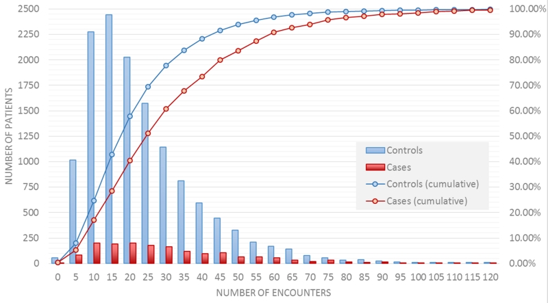
An estimate of the data density (i.e., in-person and phone encounters) in the observation window (set at two years for this analysis) is computed for each case and control by first accounting for each instance of a diagnoses, medications, labs, imaging orders and vitals data types along with the associated date.. Next, the total number of distinct dates is computed. This “number of encounters” is then used as the data density estimate. A total of 18% of cases (red line, figure 7) and 25% of controls (blue line, Figure 7) had less than 10 encounters. Half of the controls have less than 20 encounters and half of the cases have less than 25 encounters.

Figure 7.

Distribution of the number of encounters in the 2 year observation window for cases and controls.

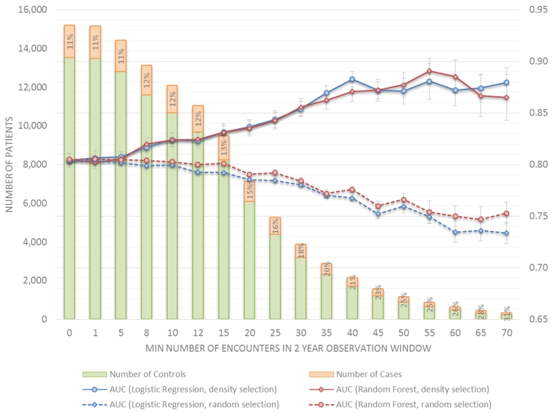
To measure prediction performance as a function of the training data density, a series of regularized logistic regression and random forest classifiers were trained and evaluated using 10-fold cross validation on different subsets of the training data selected using two methods: 1) based on increasing data density in the observation window and 2) randomly without replacement to meet a specified data set size. The density based selection was performed by including case and control patients that have at least the minimum number of specified encounters in the 2 year observation window. The bar graphs in Figure 8 show that as the density threshold increases, the number of selected cases (red bars) and controls (blue bars) that have the minimum number of required encounters in the observation window decreases. Each bar graph is labeled with a percent of the total patients who are cases, where cases comprise 11% of all patients. This percentage changes slightly when both case and control patients are restricted to those with 10 or more encounters in the observation window (i.e., 12% to 13%), then increases incrementally to 15% at 20 encounters and finally to 26% at 60 encounters. The green curve in Figure 8 plots the mean and standard error of the cross validated AUC scores (vertical axis) as a function of the data set density (horizontal axis) expressed as the minimum number of encounters in the observation window. Predictive performance improves significantly when data are restricted to those with at least 10 to 15 encounters in the 2 year observation window, a range where the exclusion of cases and controls is similar. Model performance continues to improve when data are restricted to those with more encounters, but the selective exclusion of controls is substantial compared to cases. As a comparative baseline, models trained using the same amount of data but selected randomly instead of by data density are evaluated. For each threshold value, 50 iterations of training and testing are performed using randomly selected data sets that are the same size as the corresponding density based data set. The purple curve in Figure 8 plots the mean (and standard error) of the 50 AUC scores for each threshold data set size. Performance holds steady for moderate data set sizes (down to 6000 patients) and then slowly drops off as the data set size decreases. These results seem to indicate the importance of having less but denser data over having more but sparser data.

Figure 8.

Prediction performance as a function of data density and data size.

Discussion

The adoption of electronic health records in US healthcare is contributing to an explosive growth in diverse longitudinal patient data that will increasingly support population level analyses to support individualized patient care. Predictive analytics represent one important domain that is relevant to early detection of disease, avoidable care (e.g., hospital admission), and clinical decision support, among numerous other applications. The quantitative performance of a predictive model, represented by the AUC, is often a dominant focus of concern, but this represents only one of several factors that will dictate the overall utility of and the likelihood that a model will be adopted for clinical care (Table 3). In this paper we explored how the quantity and diversity of EHR data influences model performance defined by both the AUC and other features. We consider implications for implementation of predictive models specifically for the early detection of heart failure and then consider issues with generalizability.

Table 3.

Model Utility in Health Care Delivery

Model performance	AUC, Sensitivity, Specificity, PPV, etc.
Data requirements	Shorter observation window, fewer features
Model coherence and translation	Transparency, interpretability, clinical and etiological utility, actionability
Model purpose and validation	Diagnosis, prognosis, risk management, risk communication, treatment/intervention indication
Ease of updating	Ease of implementation, platform utilities
Ease of use/access	User access, requirements, and burden; Integration with workflow

The demand for more diverse, voluminous, or higher density of data to improve model performance creates an inevitable tension by reducing the size of the market that can use the model. This tension does not necessarily lead to the creation of a single model that is designed to the lowest common denominator. Rather, the tradeoff influences the family of models that might be created to accommodate differences in the data that are available to specific provider groups. In our analysis, model performance was most strongly influenced by the diversity of data, basic feature construction, and the length of the observation window. In raw form, EHR data are highly diverse, represented by thousands of variants for disease coding, medication orders, lab measures and other data types. It seems obvious that some level of feature construction that relies on well-established ontologies should improve model performance. We examined this specific issue because it had not been previously explored. Use of ontologies for ICD-9 codes and medication classes each substantially improves model AUC, reduces the number of features, or both. Modest curation of data using existing ontologies substantially reduces data diversity without loss of information and possibly a gain in information that both supports improvement to model performance, parsimony, and coherence. Moreover, this modest data curation also simplifies standardization of data across different provider entities. This finding may suggest that more advanced forms of data curation that are beyond traditional ontologies may further improve model performance and parsimony.

The adoption of predictive models will depend, in part, on the data diversity requirements Adoption is more favorable when the same or similar model performance can be achieved with fewer types of data. In our analysis, model performance was considerably better when using either diagnoses or medication order data alone compared to other data types (i.e., labs, hospitalization, demographics/health behaviors, image orders, and vitals). These two domains may be dominant because they also represent the most common sources of data and also offer information relative to a patient’s status over a longer period of time than a clinical measure. This does not necessarily mean that larger quantities of lab or vital sign data that could be generated from wearable devices could also improve model performance for those specific domains. Notably, the combination of diagnoses, medications, demographics/health behaviors, and vital sign data does not yield an AUC that is significantly better than diagnoses and medication data alone (i.e., AUC of 0.752 versus 0.740, p=0.23, data not shown). While we cannot generalize to predicting other health problems, the findings are sensible given that information about smoking and alcohol use habits and vital signs are likely to be captured by diagnoses and medication data. For example, ICD-9 codes for hypertension combined with related medication orders may be more informative than intermittent measures of blood pressure. One limitation to our assessment of data types is related to the image order data. Other than ECHO order data on LVEF we did not extract test results for other imaging orders.

We examined a 12-month prediction window, varying the length of the observation window. While a longer observation window increases the volume of data it also reduces the number of patients to whom the model could be applied in a given provider group. Not surprisingly, model performance improved substantially as the length of the observation window increased. Performance began to plateau for observation windows longer than two years. For HF this finding may suggest that signals of early detection in EHR data may only exist within one to three years of diagnosis. However, in modeling experiments, the observation window was treated as a static dataset represented by summary statistics. It is possible that longer observation windows improve model performance when using more advanced models that can make temporal connections among features or events.

The most surprising finding in this study is how sensitive the model performance is to the size of the training set. Substantial improvements to our predictive model were achieved by increasing the training set size from 1000 patient records to 4000 records. While the training set size may be influenced by other factors (e.g., type of data, case/control ratio, data density), this finding, in particular, may pose the greatest challenge to application of models in clinical practice. It is likely that any predictive model that is developed for use in clinical practice will have to be adapted to the data available in a clinical practice. That is, model development work largely offers a guide on data requirements and data curation, not the specific formulation that could be applied to patient data. As such, the training set size may be the most influential factor in adoption of predictive models for smaller practice groups. The case-control dataset for this study included 1,684 HF cases and 13,525 controls from a modest size clinical practice. The incident HF cases accrued over a 7-year period. It is unlikely that most practice groups will have equivalent or greater denominators, represented by the combination of years of data and size of the patient population. While we do not have evidence of the generalizability of this finding to other areas of predictive modeling, we can conclude that there is likely to be a strong tradeoff in model performance and the size of the training set and that smaller practices may benefit from pooling of data.

The quantity and diversity of available EHR data are highly heterogeneous among patients and this poses potential methodological challenges in using EHR data for predictive modeling purposes. In contrast to epidemiological data that are collected using a structured protocol and time schedule, EHR data accrue in an unscheduled manner and with a modest amount of structure defined by clinical protocols. For example, vital signs are collected during most visits, but often with variation in the “protocol.” The frequency, type and quantity of lab tests ordered can also be widely inconsistently among practitioners and their patients. Other data like ICD-9 codes and medication orders are documented using standardized schemes, but physicians vary in how they document and what they order. Patients also vary in how much care they use, independent of disease burden. In our analysis, we found that data density strongly influences model performance. Using a two-year observation window and one-year prediction window, model performance substantially improved when a minimum of 10 encounters was required, but even at these thresholds 20% or more of patients in a primary care practice would be excluded from risk assessment using the HF model. Performance continues to improve by restricting the data to patients with more than 15 encounters. In this experiment, the number of encounters between cases and controls are matched. As such, the performance gain cannot be explained by the difference in number of encounters between cases and controls. Some of the improvement may be due to a better representation of the patient derived from more data. Some of the additional gains in AUC may be due to the larger fraction of cases compared to controls being selected with higher density threshold values. More work needs to be done to better understand this behavior. Since some individuals who develop HF do so after a singular acute event, such as following a heart attack or a viral cardiomyopathy, there are likely to be a subset of people whose HF diagnosis follows a much more rapid trajectory and are more likely to have fewer medical encounters in the months to years before their diagnosis.

Several features (i.e., alpha/beta blockers orders, positive JV distention, negative pulmonary edema, loop diuretic orders, cardiac disorders) in the final model (Table S1) may suggest a covert HF diagnosis, but this does not necessarily mean that HF is actually present or even that individuals with those features will develop HF. The predictive importance of a feature (Table S2) takes into account both the discriminability and frequency of the variable. Features that may indicate HF often ranked relatively low in importance (e.g., positive JV distension ranked 97th, alpha/beta blockers ranked 89th, negative pulmonary edema ranked 46th). When these five features were eliminated from the model the AUC was only reduced from 0.796 to 0.785. More importantly, there is considerable “noise” in EHR data and it is very difficult to state with certitude that an individual patient is at risk of a future diagnosis of HF simply because these features appear in their record. For example, Framingham HF signs and symptoms were common among cases and controls and had relatively little impact on model performance. Predictive models offer the means to discriminate the meaning of thousands of data points that simply cannot be deciphered by manual review. Moreover, even if a patient had HF before the recorded diagnosis date, the patient is not being managed accordingly. The value of predictive models in this context is to offer the means to conduct routine surveillance to surface and more effectively manage these patients before they are hospitalized for the first time with HF.

Our findings are consistent with prior work using EHR data. In predicting mortality over different time horizons from end-stage renal disease (ESRD), machine learning models that contain all available predictors outperform those that do not [18]. But, variable groups varied by utility, where exclusion of any particular group did not lead to a meaningfully reduction in risk prediction. Moreover, prediction performance decreased as the prediction window size increased (from 1 day to 3 years). Separately, renal function disease progression was modeled using machine learning methods with and without temporal information on data features. Prediction performance improved for temporal and non-temporal models as the observation window size increased with peak performance occurring between 2 and 3 years of patient data [19]. In a different study, significant differences in the accuracy of hypoglycemia prediction using machine learning models for patients with type 2 diabetes were observed as a function of data density (number of self-monitored blood glucose data points) and prediction window size (1 hour to 24 hours) [20]. Model performance increased with denser data and with smaller prediction window size. There are a number of possible directions for future work. First, the approach and methods need to be validated on larger patient data sets from multiple healthcare systems and additional disease targets to better understand the generalizability of the data characteristic impacts on predictive modeling performance. More in depth analysis of the characteristics and distribution of the top risk factors captured by the predictive model is also needed. In this study, the prediction and observation windows were explored separately; understanding the combination of them is also important. Exploration of novel approaches to data curation that rely on combinations of data elements to characterize variation in disease complexity, disease control, and other features may improve model performance or coherence or both. It will be important to explore data density, training set size, and other requirements in greater depth and to develop methods that reduce the data demands as a means to increase adoption. Finally, use of modeling strategies that account for the sequencing and temporal distance of features in the observation window may offer an approach to increase model performance with the same amount of data.

What is Known.

• -Electronic health records (EHR) data can be used to predict events including onset of diseases but there is little known about the practical tradeoffs between data requirement and model utility.
• -Rapid growth in the application of machine learning methods to EHR for predicting future patient outcomes is fostering a deeper understanding of modeling best practices.

What the Study Adds.

• -Detailed characterization of the practical tradeoffs between data requirements and model utility is possible and shows the value and limitations of heterogeneous data sources to predictive models in EHR data.
• -Possible guidelines for the minimum amount and type of data needed to train effective disease onset predictive models using longitudinal EHR data.

References

- [1].Mozaffarian D, Benjamin E, Go A, Arnett D, Blaha M, Cushman M, Das S, deFerranti S, Després J-P, Fullerton H, Howard V, Huffman M, Isasi C, Jiménez M, Judd S, Kissela B, Lichtman J, Lisabeth L, Liu S, Mackey R, Magid D, McGuire D, Mohler E, Moy C, Muntner P, Mussolino M, Nasir K, Neumar R, Nichol G, Palaniappan L, Pandey D, Reeves M, Rodriguez C, Rosamond W, Sorlie P, Stein J, Towfighi A, Turan T, Virani S, Woo D, Yeh R, Turner M. Heart Disease and Stroke Statistics—2016 Update: A Report From the American Heart Association. Circulation. 2015;133:38–360. doi: 10.1161/CIR.0000000000000350. [DOI] [PubMed] [Google Scholar]
- [2].Roger V, Weston S, Redfield M, Hellermann-Homan J, Killian J, Yawn B, Jacobsen S. Trends in heart failure incidence and survival in a community-based population. JAMA. 2014;292:344–350. doi: 10.1001/jama.292.3.344. [DOI] [PubMed] [Google Scholar]
- [3].Murphy S, Xu J, Kochanek K. Deaths: final data for 2010. Natl Vital Stat Rep. 2013;61:1–117. [PubMed] [Google Scholar]
- [4].Wang Y, Ng K, Byrd R, Hu J, Ebadollahi S, Daar Z, deFilippi C, Steinhubl S, Stewart W. Early detection of heart failure with varying prediction windows by structured and unstructured data in electronic health records; Conf Proc IEEE Eng Med Biol Soc., EMBC.; 2015; pp. 2530–2533. [DOI] [PMC free article] [PubMed] [Google Scholar]
- [5].Vijayakrishnan R, Steinhubl S, Ng K, Sun J, Byrd R, Daar Z, Williams B, deFilippi C, Ebadollahi S, Stewart W. Prevalence of heart failure signs and symptoms in a large primary care population identified through the use of text and data mining of the electronic health record. J. Card. Fail. 2015;20:459–464. doi: 10.1016/j.cardfail.2014.03.008. [DOI] [PMC free article] [PubMed] [Google Scholar]
- [6].Byrd R, Steinhubl S, Sun J, Ebadollahi S, Stewart W. Automatic identification of heart failure diagnostic criteria, using text analysis of clinical notes from electronic health records. Int J Med Inform. 2014;83:983–992. doi: 10.1016/j.ijmedinf.2012.12.005. [DOI] [PMC free article] [PubMed] [Google Scholar]
- [7].Sun J, Hu J, Luo D, Markatou M, Wang F, Edabollahi S, Steinhubl S, Daar Z, Stewart W. Combining knowledge and data driven insights for identifying risk factors using electronic health records. AMIA Annu Symp Proc. 2012:901–910. [PMC free article] [PubMed] [Google Scholar]
- [8]. [Accessed: 04-Feb-2016];Epic: Software. Online. Available: http://www.epic.com/software-index.php.
- [9].Gurwitz J, Magid D, Smith D, Goldberg R, McManus D, Allen L, Saczynski J, Thorp M, Hsu G, Sung S, Go A. Contemporary prevalence and correlates of incident heart failure with preserved ejection fraction. Am. J. Med. 2013;126:393–400. doi: 10.1016/j.amjmed.2012.10.022. [DOI] [PMC free article] [PubMed] [Google Scholar]
- [10].Ather S, Chan W, Bozkurt B, Aguilar D, Ramasubbu K, Zachariah A, Wehrens X, Deswal A. Impact of Noncardiac Comorbidities on Morbidity and Mortality in a Predominantly Male Population With Heart Failure and Preserved Versus Reduced Ejection Fraction. J Am Coll Cardiol. 2012;59:998–1005. doi: 10.1016/j.jacc.2011.11.040. [DOI] [PMC free article] [PubMed] [Google Scholar]
- [11].Austin P, Tu J, Ho J, Levy D, Lee D. Using methods from the data-mining and machine-learning literature for disease classification and prediction: a case study examining classification of heart failure subtypes. J Clin Epidemiol. 2013;66:398–407. doi: 10.1016/j.jclinepi.2012.11.008. [DOI] [PMC free article] [PubMed] [Google Scholar]
- [12].Rosamond W, Chang P, Baggett C, Johnson A, Bertoni A, Shahar E, Deswal A, Heiss G, Chambless L. Classification of heart failure in the atherosclerosis risk in communities (ARIC) study: a comparison of diagnostic criteria. Circ Heart Fail. 2012;5:152–159. doi: 10.1161/CIRCHEARTFAILURE.111.963199. [DOI] [PMC free article] [PubMed] [Google Scholar]
- [13].Pope G. Evaluation of the CMS-HCC Risk Adjustment Model. CMS; 2011. [Google Scholar]
- [14].Brieman L. Random Forests. Machine Learning. 2001;45:5–32. [Google Scholar]
- [15].Bishop C. Pattern Recognition and Machine Learning. Springer; New York: 2007. [Google Scholar]
- [16]. [Accessed: 22-Feb-2016];Welcome to Python.org. Online. Available: https://www.python.org/
- [17].R Development Core Team . R: A language and environment for statistical computing. R Foundation for Statistical Computing; Vienna, Austria: 2008. [Google Scholar]
- [18].Goldstein B, Pencina M, Montez-Rath M, Winkelmayer W. Predicting mortality over different time horizons: which data elements are needed? J Am Med Inform Assoc. 2016 doi: 10.1093/jamia/ocw057. pii:ocw042. Ahead of print. [DOI] [PMC free article] [PubMed] [Google Scholar]
- [19].Singh A, Nadkarni G, Gottesman O, Ellis S, Bottinger E, Guttag J. Incorporating temporal EHR data in predictive models for risk stratification of renal function deterioration. J Biomed Inform. 2015;53:220–228. doi: 10.1016/j.jbi.2014.11.005. [DOI] [PMC free article] [PubMed] [Google Scholar]
- [20].Sudharsan B, Peeples M, Shomali M. Hypoglycemia prediction using machine learning models for patients with type 2 diabetes. J Diabetes Sci Technol. 2015;9:86–90. doi: 10.1177/1932296814554260. [DOI] [PMC free article] [PubMed] [Google Scholar]
Associated Data
This section collects any data citations, data availability statements, or supplementary materials included in this article.