Rapid automated landmarking for morphometric analysis of three‐dimensional facial scans

Abstract

Automated phenotyping is essential for the creation of large, highly standardized datasets from anatomical imaging data. Such datasets can support large‐scale studies of complex traits or clinical studies related to precision medicine or clinical trials. We have developed a method that generates three‐dimensional landmark data that meet the requirements of standard geometric morphometric analyses. The method is robust and can be implemented without high‐performance computing resources. We validated the method using both direct comparison to manual landmarking on the same individuals and also analyses of the variation patterns and outlier patterns in a large dataset of automated and manual landmark data. Direct comparison of manual and automated landmarks reveals that automated landmark data are less variable, but more highly integrated and reproducible. Automated data produce covariation structure that closely resembles that of manual landmarks. We further find that while our method does produce some landmarking errors, they tend to be readily detectable and can be fixed by adjusting parameters used in the registration and control‐point steps. Data generated using the method described here have been successfully used to study the genomic architecture of facial shape in two different genome‐wide association studies of facial shape.

Introduction

Genetic or developmental studies of morphology increasingly require phenotypic analysis of large datasets. Traditionally, analyses of morphology have relied heavily on manual measurements, for which inter‐observer error, drift in landmarking error over time and labour‐intensity present major challenges (Percival et al. 2014; Hallgrimsson et al. 2015). Three‐dimensional (3D) imaging technology has progressed rapidly, but the development of tools for standardized high‐throughput analysis of morphological data generated through imaging has lagged by comparison (Hallgrímsson & Jones, 2009; Houle et al. 2010). The rapid diversification of 3D imaging techniques, such as micro‐magnetic resonance imaging (MRI), optical projection tomography and structured white light imaging, has exacerbated the gap between imaging and morphometric data. Three‐dimensional imaging presents procedural and throughput challenges for manual landmarking (Simon & Marroig, 2015), and the increasing diversity of imaging modalities is a challenge for data standardization. One solution to increase both data throughput and consistency is the development of robust methods for automated landmarking of 3D image data for morphological analyses (Hutton et al. 2000).

Though some automated 3D landmarking methods have been available for a decade and a half (Brett & Taylor, 2000), these methods have rarely been used for large‐scale studies (Hallgrimsson et al. 2015) as they are either too computationally intensive to be practical or they violate key assumptions of landmark‐based geometric morphometrics, the most widely used approach to quantify variation in 2D and 3D biological shape and form (shape and size; Mitteroecker & Gunz, 2009). Beyond precision and repeatability, two key requirements for landmark‐based geometric morphometric analyses are as follows.

1. The landmarks are homologous across individuals; i.e. each landmark encodes the same feature in different individuals or specimens (Bookstein, 1991).

2. Each landmark represents an independent observation not determined from its relations to other landmarks (Bookstein, 1991). When this assumption is violated, dependencies among landmarks can be taken into account, but only when isolated to particular dimensions of variation (Gunz et al. 2005).

Currently, there are few broadly applicable, fully automated tools for 3D landmarking that meet these data requirements for geometric morphometric analysis (Houle et al. 2010). Existing tools for automated or semi‐automated landmarking have been applied to 2D images of Drosophila wings (Houle et al. 2003), 3D images of teeth of primates and humans (Boyer et al. 2011), and 3D human facial shape using a combination of morphological and textural features (Guo et al. 2013). A method of 3D landmarking based on facial surface data has been reported (Liang et al. 2013), but has not been applied to the large‐scale analysis of facial shape data to our knowledge.

Here, we report the development of an efficient, fully automated method for landmarking 3D human facial meshes that meets the requirements of landmark‐based geometric morphometrics, is based solely on morphology, and is sufficiently robust and rapid that it can be applied to the analysis of very large datasets. By fully automated, we mean that this method does not require the interactive definition of initial landmarks or any manual orientation of the image prior to processing. We describe and validate use of this method for quantifying morphological variation in human faces, but it is potentially applicable to image data for other anatomical structures. Our method has been successfully applied to the analysis of large datasets (N > 10 000) of human faces scans (Cole et al. 2016, in press; Shaffer et al. 2016). Here, we describe the method in detail and present rigorous validation analyses, comparing automated vs. manual landmarks of the same face surfaces, and determining the extent to which our automated landmarking method captures biological variation comparable to that obtained through manual landmarking.

Materials and methods

Overview

We developed the automatic landmarking method described below to facilitate a large genome‐wide association study of the genetic basis of facial form based on the set of facial landmarks described in Table 1 and depicted in Fig. 1. These same landmarks have been used for the genome‐wide association study of facial shape (Cole et al. 2016; Shaffer et al. 2016). Our method involves four key elements, as follows.

Table 1.

Landmark definitions

Landmark number	Landmark name	Description
1	Nasion	Midline point where the frontal and nasal bones contact (nasofrontal suture)
2	Pronasale	Midline point marking the maximum protrusion of the nasal tip
3	Subnasale	Midline point at the junction of the inferior border of the nasal septum and the cutaneous upper lip – the apex of the nasolabial angle
4	Labialesuperius	Midline point of the vermilion border of the upper lip at the base of the philtrum
5	Stomion	Midpoint of the labial fissure
6	Labialeinferius	Midline point of the vermilion border of the lower lip
7	Sublabiale	Midpoint along the inferior margin of the cutaneous lower lip (labiomental sulcus)
8	Gnathion	Midline point on the inferior border of the mandible
9	Endocanthion (right)	Apex of the angle formed at the inner corner of the palpebral fissure where the upper and lower eyelids meet
10	Endocanthion (left)	Same as 9
11	Exocanthion (right)	Apex of the angle formed at the outer corner of the palpebral fissure where the upper and lower eyelids meet
12	Exocanthion (left)	Same as 11
13	Alare (right)	Most lateral point on the nasal ala
14	Alare (left)	Same as 13
15	Alar curvature point (right)	Most posterolateral point on the alar cartilage, located within the crease formed by the union of the alar cartilage and the skin of the cheek
16	Alar curvature point (left)	Same as 15
17	Subalare (right)	Point located at the lower margin of the nasal ala, where the cartilage inserts in the cutaneous upper lip
18	Subalare (left)	Same as 17
19	Crista philtri (right)	Point marking the lateral crest of the philtrum at the vermilion border of the upper lip
20	Crista philtri (left)	Same as 19
21	Chelion (right)	Point marking the lateral extent of the labial fissure
22	Chelion (left)	Same as 21
23	Tragion (right)	Point marking the notch at the superior margin of the tragus, where the cartilage meets the skin of the face
24	Tragion (left)	Same as 23
25	Superior alar groove (right)	Most superior portion of alar groove
26	Superior alar groove (Left)	Same as 25
27	Zygion (Right)	Most prominent portion of zygomatic arch
28	Zygion (Left)	Same as 27
29	Pogonion	Most prominent portion of chin, anatomical pogonion

Figure 1.

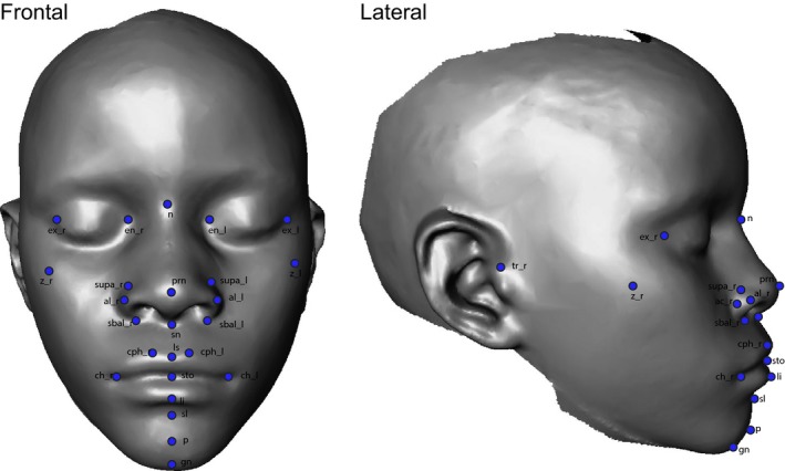
Landmarks used for morphometric analysis of facial shape.

1. Automatic alignment of individual faces prior to landmark identification.

2. A technique to automatically annotate homologous control points on facial surface meshes.

3. A small training set (n = 50) of facial meshes was manually landmarked and used to create a facial atlas of landmarks and a curvature map. The facial atlas represents a mean face from this sample. A sample, rather than an individual, is used to determine values for curvature thresholds. We use these to identify control points, which register each face to the atlas.

4. Given a facial mesh to be landmarked, the identified control points are used to register the template atlas to each mesh and subsequent transformation of the landmarks from the template to the subject.

The proposed method was developed and evaluated using 3D facial scans obtained using the Creaform^® (Québec, Canada) Megacapturor and Gemini 3D camera systems. These cameras use a structured white light method to estimate a 3D surface (Rocchini et al. 2001). In principle, however, the method can be applied to 3D surface data from various imaging modalities such as anatomical MRI or computer tomography scans. The methods behind these steps are described in more detail below.

Adjusting position and orientation

To aid automated location of the initial set of control points, we automatically position and orient each facial surface mesh into a common reference space. This is done via the following steps.

1. Highlighting features. We estimate the mean curvature at every point of the surface mesh using the algebraic point set surfaces method (Guennebaud & Gross, 2007). After this, two thresholds τ_{c_min} and τ_{c_max}, are applied to the curvature values of all points of the mesh so that the subsequent analysis steps can be restricted to points with high surface curvature (strong negative < τ_{c_min} or strong positive > τ_{c_max}). Figure 2a shows the result of the thresholding with two point clouds L ⁻ and L ⁺ coloured in blue and green, respectively. We let L be the union L ⁻∪L ⁺, so that L comprises all points with high surface curvature.

   Figure 2.

   

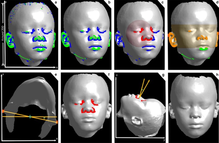   Bringing a 3D facial mesh to a standardized frontal view. (a) Curvature thresholds are applied to highlight facial features (b) and outliers are removed. (c, f) Inner orbital and nasal regions (d) and ears are coarsely identified. (e, g) Translations and rotations guided by the segmented domains are applied iteratively to (h) adjust position and orientation.

2. Removing outliers. The point cloud L coarsely delineates important key areas such as nose, lips, eyes and ears. However, it also includes points that are not associated with any well‐defined facial feature but are mostly caused by noise. To remove these outliers, a connected component analysis is performed. More precisely, the number of connected points with a curvature value below or above the corresponding curvature thresholds is counted for each component, and components smaller than τ_N are excluded from L. Figure 2b shows the corrected version of L that is obtained with this technique.

3. Segmenting eyes and nose. Let [x _min, x _max], [y _min, y _max] and [z _min, z _max] be the range of values for the x‐, y‐ and z‐coordinates of points in the facial surface mesh K. The face midpoint m is then defined by m _x= (x _min+ x _max)/2, m _y= (y _min+ y _max)/2 and m _z= (z _min+ z _max)/2. To obtain a rough segmentation of the eyes, all points p(x, y, z) in L ⁻ (negative curvature) with z < m _z (above the centre) and (x − m _x)²+ (y − m _y)²> r ² (within a radius of m _x, m _y the midpoint in x‐ and y‐directions) are removed. The result of this processing step is a coarse segmentation of the eyes and nose, which are coloured in red in Fig. 2c. In this step, we use L ⁻ because this yields a more robust segmentation due to the typical shape of eyes.

4. Orientation about the y‐axis. Let c = (c _x, c _y, c _z) be the centroid of the region segmented in the last step. The centroid is used to analyse the points in L ⁺ in the region between the planes y = c _y− α and y = c _y+ α (Fig. 2d), whereas the point with the minimum x‐coordinate is defined as p and the point with the maximum x‐coordinate as q. These two points are then used to perform a rotation centred at (p + q)/2 about the y‐axis so that the p−q segment is parallel to the x‐axis (Fig. 2e).

5. Final orientation. For final orientation, the third step (‘segmenting eyes and nose’) is repeated again to obtain a refined segmentation of the eyes and nose (Fig. 2f). Let M ₁ be the resulting point cloud of the refined segmentation. The point cloud M ₁ is then used for a principal component analysis (PCA). Experiments have shown that the third is consistently almost parallel to the z‐axis. Therefore, a rotation around the centroid of M ₁ with axis of rotation parallel to the x‐axis is performed so that the z–y slope of the third is modified to an arbitrarily defined value β = 0.175. This processing step corrects for upward or downward tilt (Fig. 2g).

6. Final position. For final positioning, the third step (segmenting eyes and nose) is repeated again. The resulting point cloud M ₂ is then used to translate the mesh by moving the centroid of M ₂ to the origin (Fig. 2h).

These steps result in the target meshes having a common position and orientation. This procedure is particular to human facial data, but similar techniques can be used to customize automated orientation and placement of other kinds of surfaces. The specific values for τ_{c_min}, τ_{c_max} τ_N, r and α were determined by application and visual analysis to a training set representing a typical range of variations of face scans.

Placement of control points and morphing

The automated placement of homologous control points on 3D facial meshes is a critical step in the landmarking process. The control points are used to align individual facial surface meshes to a common reference space, which ultimately enables a transfer of landmarks from a facial atlas template to a specific face. We employed 17 control points required for the fine registration of the template atlas to an individual face surface mesh, illustrated in Fig. S1. The method assumes that the scale and spatial orientation of all facial meshes are coarsely aligned as described above and depicted in Fig. 2.

Once the control points are identified (see Appendix S1 for details), the mean face derived from the training set is morphed to each subject using the thin‐plate spline (TPS) algorithm (Meinguet, 1979; Bookstein, 1989; Wahba, 1990) guided by the control points. The landmarks on the template atlas are then transferred to their respective closest points on the subject mesh through the TPS interpolant, yielding the desired automated facial annotations. After morphing, the landmarks defined on the mean face atlas template can be transferred to the subject, and their x, y, z coordinates are recorded for further statistical analysis. Note that the template atlas will impact the mean landmark placements in the sample, but the landmark values for every individual are determined by the morphing of each individual from the template back to its original configuration. Our training set of 50 individuals provides a reasonable estimate of the sample mean.

Validation

We validated the results of the method using two different approaches. In the first approach, we assumed manual landmarking to be the ‘gold standard’. In this test, the automated and manual methods were both used to landmark exactly the same image for each individual based on a sample of 30 facial surface meshes. Measurement deviations were calculated relative to the mean of the two measurement trials. We also estimated measurement and among‐landmarking error in 20 faces that were landmarked four times on different days, each by two different observers (total of eight trials per face).

In the second approach, to determine the extent to which the two methods capture comparable variation structure, we used partial least squares (PLS) analysis to compare covariation structure between the automated data and the manual data (using the mean of the two manual landmarking trials), using the same sample of 79 individuals used for the second experiment.

Measurement errors in automated landmarking are difficult to detect in the absence of multiple independent imaging trials, which are impractical for large studies or in clinical settings where there may not be time for completely independent trials. To determine the extent to which automated and manual landmarking generate comparable extreme errors, we used the entire dataset of automated (N = 6098) and manually landmarked (N = 300) individuals and analysed the distributions for significant outliers.

All analyses were performed in r using the Geomorph (Adams et al. 2014), Morpho (https://github.com/zarquon42b/Morpho) and BlandAltmannLeh (http://www-users.york.ac.uk/~mb55/meas/ba.htm), as well as packages for graphing (ggplot, corrplot) and 3D visualization (shapes https://cran.r-project.org/web/packages/shape/shape.pdf). Analyses of morphological variation were performed using geometric morphometric methods, and direct comparisons of methods followed the Bland–Altman approach (Altman & Bland, 1983). This method quantifies the level of agreement between two methods by plotting the differences between two measures against their average. This approach is preferable to using a correlation or regression because those metrics are influenced by the variance of the sample used to assess the methods. High correlations can occur between methods when they are poorly reproducible when the validation sample has a high variance. The Bland–Altman method reveals this when it occurs. To compare overall shape variation among groups, we used a multivariate analysis of variance (manova) as implemented in Geomorph (ProcD.lm; Collyer et al. 2015).

All of the data used for validation of our method are from the genome‐wide association study of facial shape in Tanzanian children (Cole et al. 2016). These subjects were imaged by our group in Tanzania under approved ethics protocols at the University of Calgary (CHREB 21741), the University of Colorado, Denver (Multiple Institutional Review Board protocol #09‐0731), and the Tanzania National Institute for Medical Research (NIMR/HQ/R8.c/Vol.1/107).

Results

Comparison of individuals landmarked with both manual and automated methods

The analysis of measurement error and observer error for manual landmarking revealed that error contributes significantly to variation in shape. manova for shape with Individual, Observer and Trial as factors showed that variation other than that which separates individuals accounted for nearly 35% of the total shape variation (Table 2). Simple measurement error accounted for only 1.5% of the shape variance, but added to that was significant drift in shape across measurement trials (1.6%) and a large among‐observer effect (7%) despite significant attempts to standardize landmark placement. Measurement and inter‐observer error for manual landmarking differ among landmarks, as shown in detail in Fig. S2. These results demonstrated that manual landmarking, particularly by multiple observers, was associated with significant measurement error.

Table 2.

manova on tangent space projected Procrustes coordinates to assess measurement error

Component	Df	SS	MS	Rsq	F	Z	P‐value
Individual	19	0.516	0.027	0.665	20.526	5.462	< 0.001
Observer	1	0.055	0.055	0.071	41.424	22.013	< 0.001
Trial	1	0.012	0.012	0.016	9.215	8.780	< 0.001
Observer × individual	19	0.035	0.002	0.045	1.395	1.516	< 0.001
Residuals	119	0.157	0.001
Total	159	0.775

To validate our automated landmarking protocol, we compared 30 individuals subjected to both manual and automated landmarking from the same facial surface meshes. To compare estimates of size across methods, we used the centroid size (CS; defined as the cube root of the squared distances from each landmark to the geometric centre of each landmark configuration). As shown in Fig. 3a, CS estimates were consistent between the two methods (r = 0.97, P < 0.0001). anova by individual between methods leaves only 1% of the total variance unexplained (df +29, F = 67, P < 0.0001). Bland–Altman comparison showed that the 95% confidence intervals for the CS estimates between methods are 6 mm relative to an average CS of about 240 mm (Fig. 3b). Most individuals fall within 4 mm for both methods.

Figure 3.

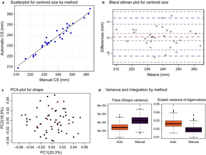
Size and shape comparison of automated and manual landmarking. (a) Regression of centroid size (CS) for the two methods. (b) Bland–Altman plot for CS. Thick blue lines show 95% confidence intervals for the difference between the methods. (c) Plot of the first two principal components (PCs) showing no difference between methods. Plots of other PCs showed similar patterns. (d) Comparison of variance and covariation for the two methods showing lower shape variance but a more tightly integrated covariance pattern for the automated landmarks.

Comparison of mean shape using manova and permutation of the Procrustes distances showed no significant differences in mean shape (P = 0.8 for manova), and PCA plots revealed no systematic differences between the manual and automated landmarking methods (Fig. 3c). The phenotypic variances, however, were significantly lower for automated compared with manual landmarking, while the covariances among landmarks were higher, as measured by the scaled variance of eigenvalues (Fig. 3d; P < 0.001). Because measurement error is likely to be normally distributed and uncorrelated among landmarks, this suggests lower error in the automated landmarking sample.

This greater variance in the manual landmarks is evident when the raw Procrustes coordinate values are plotted on the mean face (Fig. 4a). For most landmarks, the differences between the manual and automated methods average < 1 mm, with a few landmarks showing mean differences of 1–2 mm (Fig. 4b). The variation in error in absolute position among landmarks is significant (anova, df = 841, F = 102, P < 0.0001), with Tragion and Zygion showing the largest magnitudes of measurement error. A Bland–Altman plot for the deviations from each individual mean plotted against the deviation of the estimate of each mean from the sample mean shows that for most landmarks the differences between methods are much smaller than the differences among individuals in the sample (Fig. 4c). From these results, we conclude that the data generated by the automated and manual landmarking methods are very similar.

Figure 4.

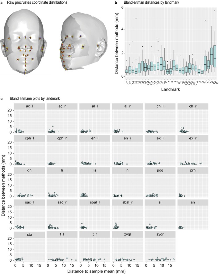
Raw distributions and error plots for comparison of automated and manual landmarking. (a) Raw Procrustes coordinate distributions for automated (blue) and manual (yellow) landmarks compared with the sample mean (red). This shows greater spread for the manual compared with automated landmarks. (b) Boxplot for the difference between methods in mm by landmark. (c) Bland–Altman plots by landmark comparing variation among individuals (x‐axis) to the difference between methods (y‐axis).

Comparison of variation structure between automated and manual landmarking

A key question is to what extent do automated and manual landmarking capture similar information about a sample? To address this, we subjected scans for 79 individuals to both manual and automated landmarking, and compared variation structure using PLS regression. Here, no homology was assumed between individual landmarks, but individuals must correspond across samples. We used the manual landmarks as the independent matrix and the automated landmarks as the response matrix. As shown in Fig. 5, the results showed a high degree of correspondence in the variation structure of the two datasets. Figure 5a shows a plot of the first PLS scores, and Fig. 5b shows the correlations for the first 40 PLS scores. The PLS analysis showed that the two methods yield variance–covariance matrices that are highly correlated (P < 0.001 based on 1000 permutations). Figure 5c shows the shape transformations that correspond to the first three PLS scores. These morphs provide qualitative confirmation that the shape variation captured through the two different methods is very similar.

Figure 5.

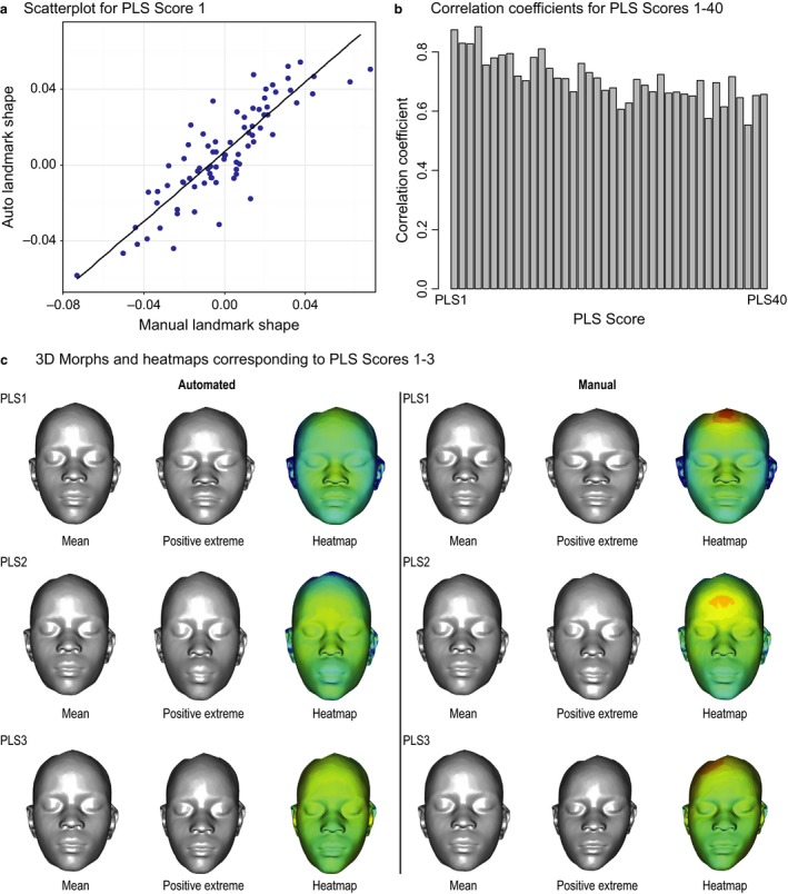
Analysis of the shape variation captured by manual and automated landmarking in 79 individuals landmarked using both the automated and manual methods. (a) The regression of the first partial least squares (PLS) scores for the two datasets. (b) Correlations for the first 40 PLS scores. (c) The shape transformations that correspond to PLS scores 1–3.

Analysis of outliers

To compare measurement errors between manual and automated landmarks, we analysed the facial image database compiled for our genome‐wide association study of Tanzanian children (Cole et al. 2016, in press); 6059 individuals were landmarked by the automated method and 366 by manual landmarking. The 366 individuals manually landmarked are the individuals identified as outliers in the analysis or that failed in the control‐point identification stage. These individuals are not a random sample, but rather those with which the automated method had the most difficulty. The landmarking program contains no stochastic elements, and so running the same images based on the same landmarking template always produces exactly the same landmark values. We verified this simply by running the landmarking program on the same image dataset twice for a sample of 3600 individuals and obtained correlations of 1.0 for all landmark values. This does not mean, however, that the program does not make any landmarking errors. To identify outliers in the automated data, we examined the relationship between two metrics. The first metric was the shape, or Procrustes, distance of each individual from the sample mean, which captures the simple mean deviation. The second metric was the variance of the shape distance of each landmark from its sample mean per individual. This metric, the landmark placement variance, captures unusual deviations at the individual landmark level. Mean deviations tend to be positively correlated across landmarks because, if a particular landmark is misplaced, this variance should be increased relative to the mean deviation. A large deviation in a particular landmark may not produce a large deviation for that whole individual.

Figure 8a shows plots of the landmark placement variance against the Procrustes distance to the mean for both automated and manual landmarking, and Fig. 6b shows histograms of the raw Procrustes distances to the mean for both automated and manual landmarking. These plots show that more extreme outliers occur in the automated dataset, and that these outliers are also characterized by large landmark placement variances. This is likely because of stepwise errors in the automated landmarking process. Such errors likely occur at the control‐point stage, such that the point that most closely matches the geometric criteria for a particular point is placed in the wrong anatomical location. When such errors occur, they need not be particularly close to the anatomically homologous point, creating discontinuous or stepwise landmarking errors. In contrast, for manual landmarking, errors are much more likely to be normally distributed.

Figure 6.

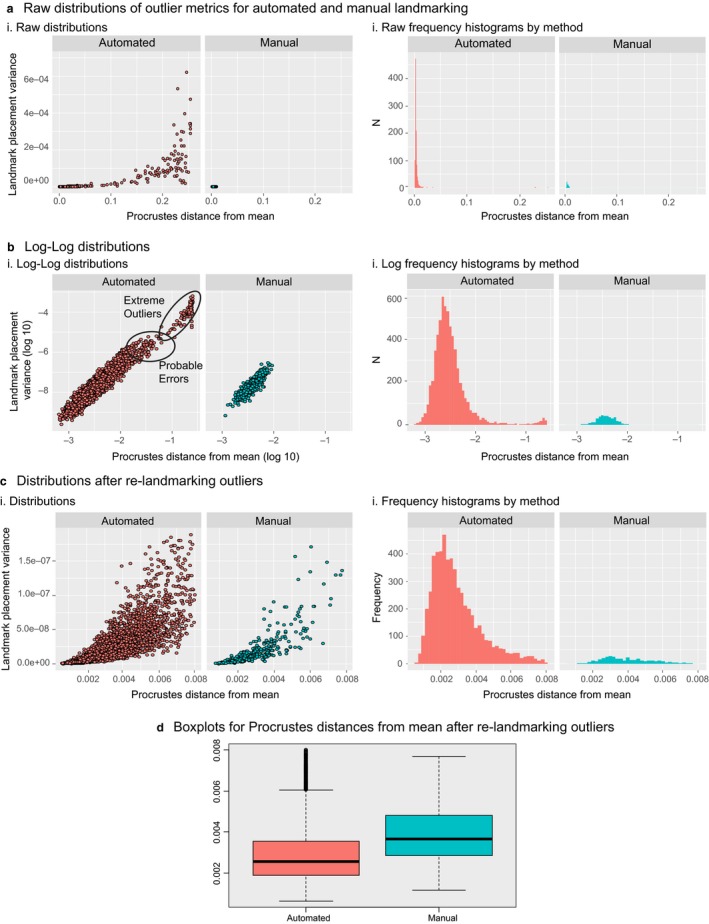
Detection and fixing of outliers in automated landmark data. (a) The distribution of outliers based on the shape distance to the mean and the landmark placement variance showing that automated landmarking tends to produce extreme outliers whereas manual landmarking does not. (b) The same data plotted on a log‐log scale. (c) These distributions after identifying and re‐landmarking the outliers identified in steps (a) and (b). (d) The shape variances and the scaled variance of eigenvalues (a measure of integration) after re‐landmarking the outliers.

This feature of automated landmarking can be used to help identify outliers. Figure 6b,c shows the same data as in Figure 6a,b, but on a log10 scale. Here, the regions of the distribution that are likely to be landmarking errors can be seen through the combination of our two outlier metrics. Inspection of the automated landmarking distribution reveals discontinuities in these distributions. Selecting the lowest of these discontinuities for both distributions eliminates about 300 individuals. Visual inspection of these individuals showed that automated landmarking had indeed produced a visible landmarking error, usually with one or more landmarks placed in the wrong location. Once these scans are removed, however, the distributions for both variables become similar for automated and manual landmarking (Fig. 8c). In this sample, the shape variance is lower for the automated sample (Fig. 8d), as is also the case in our small initial test sample.

These results show that automated landmarking can generate large measurement errors. Our results also suggest, though, that most such errors can be readily detected. The fraction of images that produce such errors will depend on the quality of the image data. Landmarking errors occurred in about 5% of the Tanzanian sample, which was obtained using two different camera systems under field conditions. All of these individuals were re‐landmarked after adjusting the parameters described in steps 1–3 above. After re‐landmarking all but nine fell within the outlier criteria after re‐landmarking, and are included in the data shown in Fig. 6d.

Discussion

Here, we present and validate a method for fully automated 3D analysis of image data. This method was developed and applied to the analysis of human faces, but the same methods can be used to create tools for automated landmarking of other anatomical structures. The shape variation obtained from automated landmarking is lower but also more highly integrated (as measured by the scaled variance of eigenvalues) compared with manual landmarks. Given that measurement error is high for manually landmarked faces, this suggests that our automated landmarking method captures biologically relevant information with lower error. Based on repeated trials, the precision of our method is very high in the sense that the same image produces the same landmark values each time. The method does, however, generate landmarking errors, and these errors are qualitatively different from those created by manual landmarking. The accuracy of automated landmarking, estimated through the Bland–Altman method, is similar to or better than those reported in studies of related methods (Subburaj et al. 2009). Most importantly, our landmarks capture variation that is very similar in structure to that obtained from manual landmarking, the ‘gold standard’. Insofar as that structure reflects underlying biological variation, automated and manual landmarking appear to capture it to very similar degrees.

Nevertheless, our validation analysis shows there are differences between the automated and manual landmarking methods that must be considered in analysis. Our initial error study of 30 facial images landmarked with both methods showed lower variances and tighter covariation for automated landmarking. This suggests lower measurement error in automated landmarking. However, analysis of the first‐pass raw landmarking data for a large sample of Tanzanian children revealed that about 5% of the images resulted in errors significantly larger than those for manual landmarking. When these apparent outliers were removed from the sample, the remaining 95% of the automated landmarking sample showed the same pattern of lower variance and tighter covariation that we saw in the initial direct comparison of manual and automated landmarks. The explanation for this result is that the automated landmarking method does result in occasional landmarking errors. Unlike with manual landmarking, however, these errors tend to be not normally distributed around the landmark mean, and instead tend to be more discontinuously distributed in magnitude due to step‐wise error in the initial control‐point identification step.

Our method also differs from manual landmarking in the use of a template. In our case, the template was based on 50 individuals from which a mean landmark configuration was obtained. Those same 50 individuals were also used to create a mean face from which the parameters used to find the controls points were extracted. For manual landmarking, accuracy is determined by the observer's knowledge of and experience with the anatomy that guides the selection of the homologous points in different individuals. Precision may be determined by multiple factors, such as image quality, resolution and the software that is used for landmarking. For automated landmarking, accuracy is determined primarily by the template, which contains the information used to assign homology across individuals. This means that an analysis of a landmark set should be based on landmarks generated using a common template. This also means that automated landmarking may miss biological information when biological homology does not correspond to geometric correspondence. There are many examples in which the relationship between geometric correspondence and homology is complex, particularly in datasets that span multiple developmental stages (Percival et al. 2014). For this reason, care must be taken when designing landmark sets or templates so as to maximize the biological information obtained from the quantification of morphology.

Precision and accuracy aside, the most compelling reason to pursue automated phenotyping methods such as the one we present here is the growing need to work with large datasets to solve increasingly complex biological problems. Integrating image data and genomics to unravel the genetics of morphological variation is one such topic that is important both in the context of human disease and the evolution of morphological diversity (Houle et al. 2010; Sozzani & Benfey, 2011; Hallgrimsson et al. 2015). Manual approaches to large datasets are too labour‐intensive and idiosyncratic to support large‐scale phenomic approaches. Even if manual landmarking by a single observer produced data of higher quality than the automated data used here, it would have been impractical to manually landmark facial scans of nearly 10 000 individuals collected over a 5‐year period. Further, many years of data collection by a human observer cannot be redone quickly if there is a need to add measurements or repeat a phenotyping task with an alternative protocol in order to compare datasets across studies. For these reasons, data quality may not be the only consideration behind the choice to use an automated rather than a manual data method of data collection.

Although we exclusively developed, tested and applied our automated landmarking method on human facial scans, it is applicable to a wide variety of 3D surface data. Future work will focus on optimizing more refined interpolation methods that can allow the method to work without the control‐point localization step. For a method that does not use control points to be fully automated, more advanced pre‐processing steps are necessary. That is because currently, hair, clothing and background in the image must be removed for the faces to be cropped in a homologous way, so that they can be registered using only the surface information itself. That would allow automated landmarking of 3D surface data to be applied to a wide variety of image data, such as from embryos and skeletal morphology. The method described here represents a significant step forward in automating the analysis of large datasets, which is critical for successfully integrating genomic and phenomic data to explore the biological basis of variation in complex morphological traits.

Supporting information

Fig. S1. Sequence of geometric constructs applied to 3D facial meshes to obtain 17 homologous anchor points.

Fig. S2. Analysis of measurement error in manual landmarks.

Fig. S3. Landmarking variation across camera systems with automated and manual landmarking.

Appendix S1. Supplementary material.

References

- Adams DC, Collyer ML, Otarola‐Castillo E, et al. (2014) Geomorph: software for geometric morphometric analyses. R package version 2.1. http://cran.r-project.org/web/packages/geomorph/index.html.
- Altman D, Bland J (1983) Measurement in medicine: the analysis of method comparison studies. Statistician 32, 307–317. [Google Scholar]
- Bookstein FL (1989) Principal warps: thin‐plate splines and the decomposition of deformations. IEEE Trans Pattern Anal Mach Intell 00, 567–585. [Google Scholar]
- Bookstein FL (1991) Morphometric Tools for Landmark Data. Cambridge: Cambridge University Press. [Google Scholar]
- Boyer DM, Lipman Y, St Clair E, et al. (2011) Algorithms to automatically quantify the geometric similarity of anatomical surfaces. Proc Natl Acad Sci USA 108, 18 221–18 226. [DOI] [PMC free article] [PubMed] [Google Scholar]
- Brett AD, Taylor CJ (2000) A method of automated landmark generation for automated 3D PDM construction. Image Vis Comput 18, 739–748. [Google Scholar]
- Cole JB, Manyama M, Kimwaga E, et al. (2016) Genomewide association study of African Children identifies association of SCHIP1 and PDE8A with facial size and shape. PLoS Genet 12, e1006174. [DOI] [PMC free article] [PubMed] [Google Scholar]
- Cole JB, Manyama MF, Larson JR, et al. (in press) Heritability and genetic correlations of human facial shape and size. Genetics. [DOI] [PMC free article] [PubMed] [Google Scholar]
- Collyer ML, Adams DC, Otarola‐Castillo E, et al. (2015) A method for analysis of phenotypic change for phenotypes described by high‐dimensional data. Heredity 115, 357–365. [DOI] [PMC free article] [PubMed] [Google Scholar]
- Guennebaud G, Gross M (2007) Algebraic Point set Surfaces. ACM Transactions on Graphics (TOG), pp. 23 New York: ACM. [Google Scholar]
- Gunz P, Mitteroecker P, Bookstein FL (2005) Semilandmarks in three dimensions In: Modern Morphometrics in Physical Anthropology. (ed. Slice DE.), pp. 73–98. New York: Kluwer Academic. [Google Scholar]
- Guo J, Mei X, Tang K (2013) Automatic landmark annotation and dense correspondence registration for 3D human facial images. BMC Bioinformatics 14, 232. [DOI] [PMC free article] [PubMed] [Google Scholar]
- Hallgrímsson B, Jones N (2009) Anatomical imaging and post‐genomic biology In: Advanced Imaging in Biology and Medicine: Technology, Software Environments, Applications. (eds Sensen CW, Hallgrímsson B.), pp. 411–426. Berlin and Heidelberg: Springer. [Google Scholar]
- Hallgrimsson B, Percival CJ, Green R, et al. (2015) Morphometrics, 3D imaging, and craniofacial development. Curr Top Dev Biol 115, 561–597. [DOI] [PMC free article] [PubMed] [Google Scholar]
- Houle D, Mezey J, Galpern P, and Carter A (2003) Automated measurement of Drosophila wings. BMC Evol Biol 3, 25. [DOI] [PMC free article] [PubMed] [Google Scholar]
- Houle D, Govindaraju DR, Omholt S (2010) Phenomics: the next challenge. Nat Rev Genet 11, 855–866. [DOI] [PubMed] [Google Scholar]
- Hutton TJ, Cunningham S, Hammond P (2000) An evaluation of active shape models for the automatic identification of cephalometric landmarks. Eur J Orthod 22, 499–508. [DOI] [PubMed] [Google Scholar]
- Liang S, Wu J, Weinberg SM, et al. (2013) Improved detection of landmarks on 3D human face data. Conf Proc IEEE Eng Med Biol Soc 2013, 1109. [DOI] [PMC free article] [PubMed] [Google Scholar]
- Meinguet J (1979) Multivariate interpolation at arbitrary points made simple. Z Angew Math Phys 30, 292–304. [Google Scholar]
- Mitteroecker P, Gunz P (2009) Advances in geometric morphometrics. Evol Biol 36, 235–247. [Google Scholar]
- Percival CJ, Green R, Marcucio R and Hallgrímsson B. (2014) Surface landmark quantification of embryonic mouse craniofacial morphogenesis. BMC Developmental Biology 14, 31. [DOI] [PMC free article] [PubMed] [Google Scholar]
- Rocchini C, Cignoni P, Montani C, et al. (2001) A low cost 3D scanner based on structured light. Computer Graphics Forum, pp. 299–308.
- Shaffer JR, Orlova E, Lee MK, et al. (2016) Genome‐wide association study reveals multiple loci influencing normal human facial morphology. PLoS Genet 12, e1006149. [DOI] [PMC free article] [PubMed] [Google Scholar]
- Simon MN, Marroig G (2015) Landmark precision and reliability and accuracy of linear distances estimated by using 3D computed micro‐tomography and the open‐source TINA Manual Landmarking Tool software. Front Zool 12, 12. [DOI] [PMC free article] [PubMed] [Google Scholar]
- Sozzani R, Benfey PN (2011) High‐throughput phenotyping of multicellular organisms: finding the link between genotype and phenotype. Genome Biol 12, 219. [DOI] [PMC free article] [PubMed] [Google Scholar]
- Subburaj K, Ravi B, Agarwal M (2009) Automated identification of anatomical landmarks on 3D bone models reconstructed from CT scan images. Comput Med Imaging Graph 33, 359–368. [DOI] [PubMed] [Google Scholar]
- Wahba G (1990) Spline Models for Observational Data. Philadelphia: SIAM. [Google Scholar]
Associated Data
This section collects any data citations, data availability statements, or supplementary materials included in this article.
Supplementary Materials