Genetic networks with canalyzing Boolean rules are always stable

Abstract

We determine stability and attractor properties of random Boolean genetic network models with canalyzing rules for a variety of architectures. For all power law, exponential, and flat in-degree distributions, we find that the networks are dynamically stable. Furthermore, for architectures with few inputs per node, the dynamics of the networks is close to critical. In addition, the fraction of genes that are active decreases with the number of inputs per node. These results are based upon investigating ensembles of networks using analytical methods. Also, for different in-degree distributions, the numbers of fixed points and cycles are calculated, with results intuitively consistent with stability analysis; fewer inputs per node implies more cycles, and vice versa. There are hints that genetic networks acquire broader degree distributions with evolution, and hence our results indicate that for single cells, the dynamics should become more stable with evolution. However, such an effect is very likely compensated for by multicellular dynamics, because one expects less stability when interactions among cells are included. We verify this by simulations of a simple model for interactions among cells.

With the advent of high-throughput genomic measurement methods, it will soon be within reach to apply reverse engineering techniques and map out genetic networks inside cells. These networks should perform a task, and, very importantly, be stable from a dynamical point of view. It is therefore of utmost interest to investigate the generic properties of networks models, such as architecture, dynamic stability, and degree of activation as functions of system size. Random Boolean networks have for several decades received much attention in these contexts. These networks consist of nodes, representing genes and proteins, connected by directed edges, representing gene regulation. The number of inputs to and outputs from each node, the in- and out-degrees, are drawn from some distribution.

It has been shown that with a fixed number, K, of inputs per node, such network models exhibit some interesting properties (1). Specifically, for K = 2, the dynamics is critical, i.e., right between stable and chaotic. Furthermore, one might interpret the solutions, i.e., fixed points and cycles, as different cell types. Being critical is considered advantageous, because it should promote evolution. These results were obtained with no constraints on the architectures and assume a flat distribution of the Boolean rules.

It appears natural to revisit the study of Boolean network ensembles, given recent experimental hints on network architectures and rule distributions. For transcriptional networks, there are indications from extracted gene–gene networks that, for both Escherichia coli (2) and yeast (3), the out-degree distribution is of power law nature. The in-degree distribution appears to be exponential in E. coli, whereas it may equally well be a power law in yeast. In ref. 4, stability properties of random Boolean networks were probed with power law in-degree distributions, and regions of robustness were identified.

The distribution of rules is likely to be structured and not random. Indeed, in a recent compilation (5) (see also ref. 6), all rules are canalyzing (1); a canalyzing Boolean function has at least one input, such that for at least one input value, the output value is fixed. It is not straightforward to generate biologically relevant canalyzing functions. In ref. 6, the notion of nested canalyzing functions was introduced, which facilitates generation of rule distributions.

We find that networks with nested canalyzing rules are stable for all power law and exponential in-degree distributions. Furthermore, as the degree distribution gets flatter, one moves further away from criticality. Also, the average number of active genes (fraction of genes that take the value “true”) is predicted for different powers.

There are experimental hints that in-degree distributions get flatter with genome size. This could be understood intuitively, because higher organisms in general have acquired more complexity in terms of redundancy in signal integration. In such a picture, our robustness analysis indicates that, with multicellular species, one would move away from critical dynamics, thereby making evolution less accessible. However, the picture is complicated by the presence of extracellular interactions. We model these with a simple scheme allowing for 5–10% extracellular traffic, and, not unexpectedly, the system, though still robust, moves toward criticality.

Methods and Models

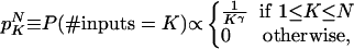
Degree Distributions. Our results turn out to be qualitatively equivalent for power law, exponential, and flat in-degree distributions. (By flat, we mean a uniform distribution for up to K_max inputs.) In what follows, we choose to illustrate the results with a power law (often denoted scale-free) distribution, with a cutoff in the number of inputs, K,

[1]

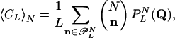
where N is the number of nodes. In yeast protein–protein networks (7) and also in other applications, e.g., the Internet and social networks, γ appears to lie in the range 2–3. In our calculations, we explore the region 0–5, varying N from 20 to infinity. The connectivity of gene–gene networks extracted from yeast (3) appears to behave like in Eq. 1 for the in-degree distributions, with an exponent γ in the range 1.5–2. For E. coli (2) data, an exponential fits somewhat better than a power law, but the data are statistically inconclusive. For mammalian cell cycle genes, slightly lower γ has been extracted (8). The average number of inputs varies with N and γ and grows with decreasing γ. For very high γ, it is essentially 1. In Fig. 1, typical network realizations for N = 20 are shown for γ = 1, 2, and 3, respectively.

Fig. 1.

Examples of N = 20 networks with γ = 1(A), γ = 2(B), and γ = 3(C).

Canalyzing Boolean Rule Distributions. In most studies of Boolean models of genetic networks, all Boolean rules have been used (1). In a previous paper (6), we introduced nested canalyzing rules and showed that it is possible to generate a distribution of such rules that fits well with rule data from the literature.

A canalyzing rule is a Boolean rule with the property that one of its inputs alone can determine the output value, for either “true” or “false” input. This input value is referred to as the canalyzing value, the output value is the canalyzed value, and we refer to the rule as being canalyzing on this particular input.

Nested canalyzing rules are a very natural subset of canalyzing rules, stemming from the question of what happens in the noncanalyzing case, that is, when the rule does not get the canalyzing value as input but instead has to consult its other inputs. If the rule then is canalyzing on one of the remaining inputs and again for that input's noncanalyzing value, and so on for all inputs, we call the rule nested canalyzing. All but 6 of the ≈150 observed rules were nested canalyzing (6).

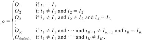
With I_m and O_m denoting the canalyzing and canalyzed values, respectively, and suitable renumbering of the inputs, i₁,..., i_K, the output, o, of a nested canalyzing rule can be expressed on the form

[2]

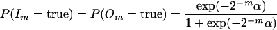
For each value of K, we generate a distribution of K-input rules, with the inputs to each rule taken from distinct nodes. All rules should depend on every input, and this dependency requirement is fulfilled if and only if O_default = not O_K. Then it remains to choose values for I₁,..., I_K and O₁,..., O_K. These values are independently and randomly drawn with the probabilities

[3]

for m = 1,..., K, where α is a constant. Eq. 3 can be seen as a way to put a penalty both on outputting true and on letting a true input determine the output. More precisely: Let f be the fraction of true outputs in the truth table, and let g be the fraction of input states such that the first input that has its canalyzing value is true. Then, the probability to retrieve a specific rule is proportional to exp[–α(f + g)/2].

Our rule distribution fits observed data well (6), given that α = 7. For all generated distributions, we keep α = 7. A high value of α means a high penalty on active genes, whereas α = 0 means equal probabilities for activity and inactivity.

Robustness Calculations. We wish to address the question of robustness in network models. In a stable system, small initial perturbations should not grow in time. In ref. 6, this was probed by monitoring how the Hamming distance H between random initial states evolved in a “Derrida plot” (9). Specifically, the slope in the low-H region shows the fate of a small perturbation after a single time step. This implicitly assumes that true and false are equally probable in the initial states.

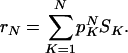
Our chosen distribution of Boolean rules will favor false node values. Preferably, a robustness measure should reflect the network properties in the vicinity of the equilibrium distribution, where the in- and out-degree distributions of true and false are identical (see Appendix A). We therefore define the robustness r_N for an ensemble of N-node networks as the average effect, after a single time step, of a small perturbation at this equilibrium distribution.

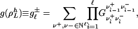
To compute r_N, we introduce the total sensitivity, S(R), of a given K-input rule R. S(R) is the sum of the probabilities that a single flipped input will alter the output of R. Thus,

[4]

where the probability is calculated over the equilibrium distribution of input values, i₁,..., i_K. Then, r is given by r =〈S(R)〉, where the average is taken over all rules in a given network (see Appendix A). This also allows us to calculate r when the rules are drawn from a distribution. Note that r is calculated without any assumption on how the inputs to the rules are chosen. This means that r stays the same for any output connectivity and for any way to build a network containing a certain set of rules. In other words, r is a strictly local stability measure that is independent of whether the network is divided into some kind of clusters or not.

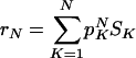
Let S_K denote the average of S(R) over a distribution of K-input rules. The average robustness of a randomly chosen network with N nodes is then given by

[5]

See Appendix A on calculation of S_K for nested canalyzing rules. With the nested canalyzing rule distribution defined by Eq. 3, S_K < 1 for K = 2, 3,..., provided that α ≠ 0. S₁ is always 1, because every rule has to depend on all of its inputs. (α = 0 yields S_K = 1 for all K.) This means that every network ensemble with the canalyzing rule distribution, and α ≠ 0, that not solely consists of one-input nodes, is stable in the sense that r < 1.

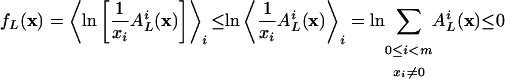
Number of Attractors. Attractors in the Boolean model can be seen as distinct cell types (1). It is, however, not straightforward to tell which attractors are biologically relevant. First, one can ask what cycle lengths are relevant. Second, the attractor basin sizes vary in a very broad range, and attractors with small attractor basins may be biologically irrelevant.

The broad distribution of attractor basin sizes also means that the number of attractors found by random sampling strongly depends on the number of samples (10).

We choose to monitor the number of attractors, 〈C_L〉_N, of different periods, L, using exact methods (for the limit N → ∞) and full enumerations of the state space (for small networks).

Given that r < 1, which means that the network is subcritical, the average number of attractors of a certain length, L, will approach a constant, 〈C_L〉_∞, as the system size, N, approaches infinity. We find an analytic expression for 〈C_L〉_∞ and find that it is qualitatively consistent with results from a full state space search for N = 20.

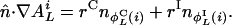
To investigate the limit N → ∞, we split up the robustness measure, r, into r^C and r^I, where r is the average number of outputs that, after one time step, will be affected by one flipped node. We define r^C and r^I as the numbers of nodes that, respectively, copy and invert the state of the flipped node. This means, e.g., that r = r^C + r^I. For convenience, we define Δr = r^C – r^I.

〈C_L〉_∞ can be expressed as a function of r_∞ and Δr_∞ for each L. For L = 1, 2, 3 we get

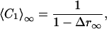[6]

[7]

[8]

See Appendix B, where the derivations needed to calculate 〈C_L〉_∞ are presented.

The canalyzing rule distribution satisfies r^C > r^I, meaning that Δr > 0. This condition yields an increased number of fixed points and attractors of odd length, compared with the symmetric case Δr = 0.

It is interesting to note that the limit of the total number of attractors,

[9]

is convergent for r < 1/2 and divergent for r > 1/2. This transition occurs at γ = 1.376, with convergence below this value. See Supporting Text, which is published as supporting information on the PNAS web site, for details.

Tissue Simulations. In multicellular organisms, we expect communication among cells to influence the network dynamics. In the real world, there exist several different types of intercellular signaling. Here we make an initial exploration using a simple model. Nevertheless, we think the results reflect some core properties.

In our model, each cell communicates with its four nearest neighbors on a square lattice with periodic boundary conditions. All cells have the same genotype and hence identical internal network architecture and rules. Each connection in the network represents how a gene product influences the transcription of some gene. Some molecules or signals can cross cell membranes and possibly diffuse far, but we consider only the case of local cell-to-cell signaling at the level of specific gene–gene interactions. Specifically, a fraction, κ, of the connections are flagged as being intercellular, and for such connections, the value is true if any of the four neighbors has true.

For the overall robustness of such tissue networks, it is not sufficient to measure the robustness r, because r depends only on interactions during a single time step, during which a perturbation can propagate only to the nearest neighbor cells. Hence, we desire a multistep robustness measure, which requires simulations, because it is outside the scope of our analysis. Rather than following trajectories from random initial states, we have chosen to identify fixed points, perturb these randomly by Hamming distance H(0) = 1, and then track the mean of H(t) for 20 time steps. In our simulations, we generate ensembles of networks using 5 × 5 lattices of cells, where each cell contains an identical network of N = 50 genes.

Results and Discussion

Three major findings emerge from Fig. 2, where the average robustness r and the fraction of active genes are shown as functions of γ in Eq. 1.

Fig. 2.

Robustness, r, and the probability of a node being true, w, at the equilibrium distribution of Boolean values, as functions of the exponent γ in the in-degree distribution p_K (Eq. 1) for N = 20 (dotted), 100 (dashed), and ∞ (solid).

1. The dynamics of the networks is always stable, regardless of the power in the in-degree distribution.

2. The stability of the networks increases with the average number of inputs to the nodes. For flatter distributions, r approaches the critical value, r = 1.

3. The average number of active genes decreases with increasing in-degree.

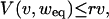
Not unexpectedly, the number of attractors increases as the networks approach criticality (see Fig. 3). This increase is particularly rapid for long cycles. These results were obtained with analytical calculation and exhaustive enumeration of state space. Given the undersampling problems when simulating Boolean networks (10), the feasibility of analytical calculations is crucial for drawing the firm conclusions above. However, we did not attempt to extract the distribution of attractor basin sizes. In future research, it could be interesting to compare this distribution to the exact results for one-input networks in ref. 11.

Fig. 3.

The number of attractors as a function of the exponent γ in the in-degree distribution p_K (Eq. 1) for N = 20 (thick lines) and N → ∞ (thin lines). The curves show the cumulative number of attractors of length L for L = 1 (solid), L ≤ 2 (dashed), and L ≤ ∞ (dotted). The values for N → ∞ were calculated analytically, whereas the values for N = 20 are taken from full enumerations of the state space for at least 5,000 networks, with more networks at higher γ.

The results in Figs. 2 and 3 are shown for power law in-degree distributions. However, they are quite general. The corresponding curves for other distributions exhibit very similar behavior, when the x axis (γ) has been transformed to appropriate parameters for other distributions. In all tested degree distributions, constant nodes (K = 0) are excluded. Recall that we also exclude rules that have redundant inputs. Thus, for low values of the average K, most of the rules will be copy or invert operators, which puts the network close to criticality. The strong stability for wide in-degree distributions, however, is a result of the canalyzing property of the rules, which makes forcing structures (1) prevalent.

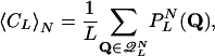
From analysis of network data from yeast (3) and the mammal cell cycle (8), there are indications that γ decreases with the number of genes. Within the framework of our results, this means that, as the genome size increases, the networks get more stable. However, with increased number of genes, multicellularity becomes common. Including interactions among cells should make the overall system less stable. Indeed, when investigating this issue by simulations of a simplified tissue model, the stability decreases with interconnectivity between the cells, κ, as can be seen from Fig. 4.

Fig. 4.

The average time evolution of perturbed fixed points in 5 × 5 cell tissues with periodic boundary conditions and N = 50 nodes (over many network realizations). Simulations from random initial states in generated networks were used to locate fixed points, which were perturbed by toggling the value of a single node. The mean distances to the unperturbed fixed point, 〈H(t)〉, as given by 20 subsequent simulation steps, are shown for γ = 2(A) and γ = 3 (B), for three different degrees of cell connectivity: κ = 0 (solid), 0.05 (dashed), and 0.1 (dotted).

We predict how the average number of active genes increases with γ. This may not be easy to verify, given that such a number will depend upon experimental conditions. It should be pointed out that the order of magnitude of active genes is set by the rule generator in Eq. 3, which is derived from fitting to the observed rules in ref. 5, many of which originate from Drosophila melanogaster. The fitted parameter α sets the scale of the fraction of active genes, with high α corresponding to low gene activity and vice versa. The qualitative behavior, however, is rather insensitive to the value of α.

Conclusion

We have designed and analyzed a class of Boolean genetic network models consistent with observed interaction rules. The emerging ensemble properties exhibit not only remarkable stability for the dynamics, but also several generic properties that make predictions, such as how stability varies with genome size, and how the number of active genes depends on the in-degree distribution. Because single-cell calculations are performed analytically, the results are transparent in terms of understanding the underlying dynamics.

Appendix A: Robustness

The stability measure r expresses the average number of perturbed nodes one time step after perturbing one node, given that the network has reached equilibrium in a mean field sense. Both the mean field equilibrium distribution (of true and false) and r are closely related to attractors in the true non-mean field dynamics (see Appendix B).

Let W(w) denote the probability that a randomly chosen rule will output true, given that the input values are randomly and independently chosen with probability w to be true. Let W_K(w) denote W(w) when the selected rule has K inputs. Then, the equilibrium probability for an N-node network, w^N_eq, satisfies

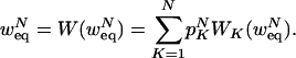[10]

Eq. 10 can be solved numerically for nested canalyzing rules, taking advantage of the fast (exponential) convergence of W_K(w) as K → ∞ and using standard (integration-based) methods to calculate the sum in the case that N → ∞. Note that w^N_eq is referring only to the mean field equilibrium distribution, which is essentially the same as, but not identical to, the distribution of true and false after many time steps in a simulation.

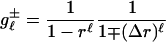
For nested canalyzing rules, W_K(w) is given by

[11]

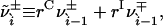
where and 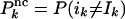. The input values, i₁,..., i_K, are true with probability w, whereas the corresponding probabilities for I₁,..., I_K and O₁,..., O_K are given by Eq. 3.

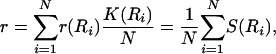
Let r(R) denote the probability that the rule R depends on a randomly picked input, given that the other inputs are independently set to true with probability . We can express r for a specific N-node network with rules R₁,..., R_N as

[12]

where K(R_i) is the number of inputs to R_i. We have defined S(R) = K(R)r(R), so that r is the average of S(R) over all rules in the network. This is also valid for a distribution of networks, meaning that

[13]

for N-node networks, where S_K is the average of S(R) when random K input rules are chosen.

Eq. 13 is exact, given that the state of the network is randomly picked from the mean field equilibrium distribution of true and false. Because the derivations are completely independent of the specific network architecture, this result holds for any procedure to generate architectures, so N long as the average fraction of nodes with K inputs are given by (over many network realizations).

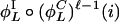
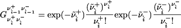
For nested canalyzing rules, we can calculate S_K as a sum of probabilities. If the rule is canalyzing on input k, and changing i_k makes the rule canalyze on input j, there is some probability that the output value changes. The case that the rule falls back to O_default corresponds to the last term in the square brackets.

[14]

where 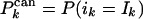and .

Let v and V(v, w) denote the fraction of input and output values, respectively, that are toggled (from false to true or vice versa) when going one step forward in time, given that the fraction true input values is w both before and after the input is toggled. Then, V(0, w) = 0, because constant input renders constant output. A small change in v will change the output with r times the change v. This means that ∂_vV(v, w_eq) ≤ r, where the inequality comes from the possibility that new changes undo previous ones as v is increasing. Combining these relations yields

[15]

which means that, for r < 1, V(v, w_eq) ≤ v with equality if and only if v = 0. Hence, frozen states, where the fraction of true nodes is w_eq, are the only solutions to the mean field dynamics, given that r < 1, which is true for the nested canalyzing rule distribution.

Note that v can be seen as the distance, i.e., fraction of differing states, between two separate time series. Then, the mapping gives the evolution of the distance during one time step. Similar calculations have been carried out in e.g., refs. 12 and 13, yielding results consistent with Eq. 15.

Appendix B: Attractors

To calculate the average number of attractors, we use the same approach as in ref. 10. This approach means that we first transform the problem of finding an L cycle to a fixed point problem, and then find a mathematical expression for the average number of solutions to that problem.

Assume that a Boolean network performs an L cycle. Then, each node performs one of 2^L series of output values. We call these L cycle series. Consider what a rule does when it is subjected to such L cycle series on the inputs. It performs some Boolean operation, but it also delays the output, giving a one-step difference in phase for the output L cycle series. If we view each L cycle series as a state, an L cycle turns into a fixed point (in this enlarged state space). L〈C_L〉_N is then the average number of input states (choices of L cycle series) for the whole network, such that the output is the same as the input.

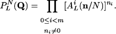
Let Q denote a specific choice of L cycle series for the network, and let be the set of all Q, such that Q is a proper cycle. A proper L cycle has no period shorter than L. The average number of L cycles is then given by

[16]

where denotes the probability that the output of the network is the same as the input Q.

Because the inputs to each K input rule are chosen from a flat distribution over all nodes, is invariant with respect to permutations of the nodes. Let n = (n₀,..., n_m–1) denote the number of nodes expressing each of the m = 2^L series. For n_i, we refer to i as the index of the considered L cycle series. For convenience, let the constant series of false and true have indices 0 and 1, respectively. Then,

[17]

where () denotes the multinomial N!/(n₀! ··· n_m–1!), and is the set of partitions n of N such that Q ∈ . That is, n represents a proper L cycle.

Let denote the probability that a randomly selected rule will output L cycle series i, given that the input series are selected from the distribution x = (x₀,..., x_m–1). Because a node may not be used more than once as an input to a specific rule, should also depend on N. However, the difference between allowing or not allowing coinciding inputs vanishes as N goes to infinity, because the output is effectively determined by relatively few inputs for nested canalyzing rules.

Because these calculations aim to reveal the asymptotic behavior as N → ∞, we allow for coinciding inputs in the following. Then, we get

[18]

By combining Eqs. 17 and 18 and applying Stirling's formula to (), we get

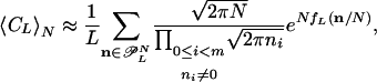[19]

where

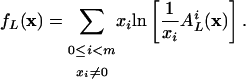[20]

See Supporting Text regarding the use of Stirling's formula.

Eq. 20 can be seen as an average 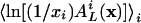with weights x₀,..., x_m–1. Hence, the concavity of yields

[21]

with equality if and only if

[22]

where . Eq. 22 can be seen as a criterion for mean field equilibrium in the distribution of L cycle series. This makes it possible to connect quantities observed in mean field calculations to the full nonmean field dynamics.

Because Nf_L(x) occurs in the exponent in Eq. 19, the relevant contributions to the sum in Eq. 19 must come from surroundings to points where Eq. 22 is satisfied as N → ∞. [f_L(x) is not a continuous function, but obeys the weaker relation “For all x, in the definition set of f_L, and ε > 0, there is a δ > 0 such that f_L(x′) < f_L(x) + ε holds for all x′ satisfying |x′ – x| < δ in the definition set of f_L.” which is a sufficient criterion in this case.] Eq. 19 provides an upper bound to 〈C_L〉_N, because the approximation of () is an overestimation (see Supporting Text). Hence, the relevant regions in the exact sum, Eq. 17, surround solutions to Eq. 22.

Given that Eq. 22 holds, the fraction of true values, w(x), and the fraction of togglings, v(x), in the distribution of L cycle series, should be consistent with the mean field dynamics, meaning that w(x) = w_eq and v(x) = 0 (see Appendix A). This means that a typical attractor, for large N, has only a small fraction (which approaches 0 for N → ∞) of active (nonconstant) nodes.

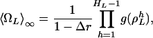
For large N, we want to investigate the number of attractors for certain numbers of active nodes. Hence, we divide the summation in Eq. 17 into constant and nonconstant patterns. To give the sum a form that can be split in a convenient way, we introduce the quantity 〈Ω_L〉_N, which we define as the average number of states that are part of a cycle with a period that divides L (see Supporting Text on how to express 〈C_L〉_N in terms of 〈Ω_L〉_N). Because N → ∞, the summation over constant patterns has a limit that yields

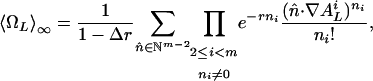[23]

where n̂ = (n₂,..., n_m–1), and denotes the set of nonnegative integers (see Supporting Text).

The elements of the gradient are nonzero only if the L cycle series i can be the output of a node that has only one nonconstant input retrieving the L cycle series j. This is true if the series j is the series i, or the inverse of i, rotated one step backward in time. Let and denote those values of j, respectively. Then,

[24]

Eq. 24 yields that the sum in Eq. 23 factorizes into subspaces, spanned by sets of L cycle series indices of the type {i, , , , ,...} containing all possible results of repeatedly applying and to i. We call those sets invariant sets of L cycle series, which is the same as invariant sets of L cycle patterns in ref. 10, but formulated with respect to L cycle series instead of L cycle patterns. Let ,..., –1 denote the invariant sets of L cycle series, where H_L is the number of such sets. For convenience, let be the invariant set {0, 1}.

Consider an invariant set of L cycle series, . Let be the length of , meaning that is the lowest number such that, for i ∈ , is either i or the index of series i inverted. If , we say that the parity of is positive. Otherwise, the parity is negative. The structure of an invariant set of L cycle series is fully determined by its length and its parity. Such a set can be enumerated on the form {,..., , ,..., } and for positive parity, whereas for negative parity.

Let strings of T and F denote specific L cycle series. Then and . Examples of invariant sets of four-cycle series are {FFFT, FFTF, FTFF, TFFF, TTTF, TTFT, TFTT, FTTT} and {FTFT, TFTF}. The first example has length 4 and positive parity, whereas the second has length 1 and negative parity.

Let , ,..., , denote the numbers, n_i, of occurrences of L cycle series belonging to , in such a way that and 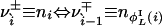. For convenience, we introduce as a renaming of . There are two ways that can be connected to : either (positive parity) or (negative parity).

Each invariant set of L cycle series, , contributes to Eq. 23 with a factor

[25]

where

[26]

[27]

and for , whereas for . Eq. 26 is interpreted with the convention that 0⁰ = 1 to handle the case where or .

Although the right-hand side in Eq. 25 looks nasty, it can be calculated, yielding the expression

[28]

(see Supporting Text).

Now, we can write Eq. 23 as

[29]

where g() is calculated according to Eq. 28. The period, , and the parity, + or –, of a given invariant set of L cycle series can be extracted by enumerating all L cycle series. This provides a method to calculate 〈Ω_L〉_∞ for small L. See Supporting Text on how to calculate 〈Ω_L〉_∞ in an efficient way.

References

- 1.Kauffman, S. A. (1993) Origins of Order: Self-Organization and Selection in Evolution (Oxford University Press, Oxford).
- 2.Huerta, A. M., Salgado, H., Thieffry, D. & Collado-Vides, J. (1998) Nucleic Acids Res. 26, 55–59. [DOI] [PMC free article] [PubMed] [Google Scholar]
- 3.Lee, T. I., Rinaldi, N. J., Robert, F., Odom, D. T., Bar-Joseph, Z., Gerber, G. K., Hannett, N. M., Harbison, C. T., Thompson, C. M., Simon, I., et al. (2002) Science 298, 799–804. [DOI] [PubMed] [Google Scholar]
- 4.Aldana, M. & Cluzel, P. (2003) Proc. Natl. Acad. Sci. USA 100, 8710–8714. [DOI] [PMC free article] [PubMed] [Google Scholar]
- 5.Harris, S. E., Sawhill, B. K., Wuensche, A. & Kauffman, S. (2002) Complexity 7, 23–40. [Google Scholar]
- 6.Kauffman, S., Peterson, C., Samuelsson, B. & Troein, C. (2003) Proc. Natl. Acad. Sci. USA 100, 14796–14799. [DOI] [PMC free article] [PubMed] [Google Scholar]
- 7.Uetz, P., Giot, L., Cagney, G., Mansfield, T. A., Judson, R. S., Knight, J. R., Lockshon, D., Narayan, V., Srinivasan, M., Pochart, P., et al. (2000) Nature 403, 623–627. [DOI] [PubMed] [Google Scholar]
- 8.Fox, J. J. & Hill, C. C. (2001) Chaos 11, 809–815. [DOI] [PubMed] [Google Scholar]
- 9.Derrida, B. & Weisbuch, G. (1986) J. Phys. 47, 1297–1303. [Google Scholar]
- 10.Samuelsson, B. & Troein, C. (2003) Phys. Rev. Lett. 90, 098701. [DOI] [PubMed] [Google Scholar]
- 11.Flyvbjerg, H. & Kjaer, N. J. (1988) J. Phys. A Math. Gen. 21, 1695–1718. [Google Scholar]
- 12.Aldana, M. (2003) Physica D 185, 45–66. [Google Scholar]
- 13.Derrida, B. & Pomeau, Y. (1986) Europhys. Lett. 1, 45–49. [Google Scholar]
- 14.Feller, W. (1968) in An Introduction to Probability Theory and Its Applications (Wiley, New York), Vol. 1, 3rd Ed., pp. 50–53. [Google Scholar]
Associated Data
This section collects any data citations, data availability statements, or supplementary materials included in this article.