Modelling turbulent boundary layer flow over fractal-like multiscale terrain using large-eddy simulations and analytical tools

Abstract

In recent years, there has been growing interest in large-eddy simulation (LES) modelling of atmospheric boundary layers interacting with arrays of wind turbines on complex terrain. However, such terrain typically contains geometric features and roughness elements reaching down to small scales that typically cannot be resolved numerically. Thus subgrid-scale models for the unresolved features of the bottom roughness are needed for LES. Such knowledge is also required to model the effects of the ground surface ‘underneath’ a wind farm. Here we adapt a dynamic approach to determine subgrid-scale roughness parametrizations and apply it for the case of rough surfaces composed of cuboidal elements with broad size distributions, containing many scales. We first investigate the flow response to ground roughness of a few scales. LES with the dynamic roughness model which accounts for the drag of unresolved roughness is shown to provide resolution-independent results for the mean velocity distribution. Moreover, we develop an analytical roughness model that accounts for the sheltering effects of large-scale on small-scale roughness elements. Taking into account the shading effect, constraints from fundamental conservation laws, and assumptions of geometric self-similarity, the analytical roughness model is shown to provide analytical predictions that agree well with roughness parameters determined from LES.

This article is part of the themed issue ‘Wind energy in complex terrains’.

1. Introduction

Modelling of atmospheric flow over complex terrain is receiving increased attention due to wind turbine siting needs. Atmospheric boundary layer (ABL) flow over complex terrain results in complex flow conditions, including unusual vertical distributions of wind shear, relatively high turbulence intensities and complicated inflow angles, all of which often affect wind turbine performance and loading. Improved prediction tools can help mitigate such issues. In that context, large-eddy simulations (LES), Reynolds-averaged modelling and analytical models that can faithfully reproduce the interactions of wind with complex terrain are desirable [1–4]. Realistic ground surfaces tend to be very rough, and roughness elements typically display a range of shape complexities and size distributions. The present contribution addresses boundary layer flow over rough surfaces, focusing on a particular complexity of roughness, namely when it is multiscale, i.e. when the roughness elements attached to the surface are characterized by a broad size distribution, covering a large range of scales. Such wide-scale distributions are a hallmark of natural and urban terrains.

Rough-wall turbulent boundary layers, in general, have received sustained attention for many decades (see reviews in [5–9]). Much attention has been focused on roughness that can be characterized by one or a few length scales. Cubes, for example, are one type of commonly studied roughness element (see e.g. [10,11] for experiment studies, [12,13] for direct numerical simulation results and [14–18] for modelling efforts). Beside cubes, in previous work single-scaled roughness elements, including pyramids [19], egg-carton-like roughness [20], ridges [21], etc., have been considered (see [9] for a review). Sand-grain-roughened pipes/channels are yet another type of rough walls of common interest (see e.g. [22–24]). Many efforts have been devoted to surfaces with roughness that can be characterized by one or a few length scales. As mentioned above, roughness in natural terrain is multiscale and, many times, assuming that it is fractal-like provides a practically useful simplification [25,26]. Recently, there has been growing interest in flow interactions with multiscale structures (see e.g. [27–31] for studies on the turbulent wake downstream of fractal obstacles, and [32–37] for wind interactions with fractal tree-like structures). Moreover, in [38,39], a dynamic approach has been developed for LES of ABL over ground roughness with power-law height spectra such as the surface shown in figure 1a, i.e. synthesized by superposing randomly phased Fourier modes.

Figure 1.

(a) Synthesized rough surface using randomly phased Fourier modes with a −1 power-law height spectrum. (b) Synthesized rough wall using self-similar rectangular roughness elements with an element number density (per unit area), N(R_n), that increases with their size R_n+1=2⁻ⁿR₁ according to .

Recent progress has been made on developing analytical roughness models (ARMs) for the case of rectangular-prism-shaped roughness elements [17]. There, based on a series of LES runs for many different cases, a fully analytical method to relate surface geometric characteristics with roughness parameters has been developed. The approach is based on the von Karman–Polhausen integral method coupled with a geometrically explicit sheltering model. While the model was relatively straightforward to formulate for rectangular-prism-shaped roughness elements, still the approach was limited to elements of similar sizes (some variability in height was considered, but the base area of elements was constant). In this study, we aim to take the approach and results from Yang et al. [17] and generalize them to the case of surfaces with broad size distributions. Specifically, we consider ground roughness with power-law size and height distributions. In order to make direct connection with the work in [17], we consider multiscale surfaces consisting of rectangular prisms. An example of such a surface is shown in figure 1b. To construct this surface, we quadruple the number of roughness elements on the ground as the sizes of the rectangular roughness elements are halved. As a result, nominally, the synthesized rough wall follows a power-law height distribution. Such roughness poses major challenges to numerical simulations and theoretical modelling.

Often roughness effects are expressed in terms of the frontal area A_f or the frontal area density λ_f=A_f/A_T, where A_T is the total planform area of the underlying surface. Clearly, as the number of scales (octaves) increases, λ_f diverges, as for a given A_T, for each new generation (octave) added, the total area added associated with each smaller and smaller element is constant (denoting the length scale of elements of the nth generation as R_n, the area of each element goes like and their numbers like ). In terms of the drag force, however, one expects the force to be finite, as flow sheltering of small elements in the wakes of large elements should avoid the divergence of the force.

It is these trends that we aim to model and address in this paper, i.e. we aim to develop modelling and simulation tools that can handle general fractal-like ground roughness distributions, including those with nominally infinite frontal area. Specifically, we first develop a numerical LES tool to handle flow over fractal-like ground roughness. With such a tool the effective hydrodynamic properties can be deduced from the simulation results. Based on these results, we also attempt to develop analytical models that can make fast and accurate predictions on roughness aerodynamic properties using only non-aerodynamic inputs.

Specifically, the paper is organized as follows. In order to generate empirical insights on flow–roughness interactions when an increasing number of scales of roughness elements are included, in §2 we conduct a series of LES. We begin with LES in which the roughness spectrum is partly resolved and no model is included to account for the effects of unresolved roughness (§2a). Next, in §2b, we aim to simulate the case where nominally we include the effects of the entire range of scales. To simulate flow over fractal-like roughness, including the full spectrum, the drag from unresolved roughness needs to be included in the LES. A possibility is to include this via specification of an effective roughness height, z_0,sg, the subgrid roughness (an LES wall closure). Compared with an ad hoc, empirical correlation, a dynamic approach that allows z_0,sg to depend on resolved flow conditions is usually preferred. Here we follow a combination of the approaches proposed in [36–38] based on the notion of scale invariance. Specifically, in order to develop a dynamic roughness model (DRM), we make the assumption that the high-Reynolds-number turbulent flow, by interacting with the geometrically scale-invariant rough surface, is itself scale-invariant. With LES grids resolving part of the roughness and the DRM modelling drag from the subgrid roughness, simulations of flow over fractal-like rough surfaces are conducted.

To deduce the aerodynamic properties of a rough wall from an LES can still be expensive, and applications like wind farm siting often need more direct methods to determine the near-wall flow conditions. In such a context, an ARM that enables one to express directly the overall aerodynamic properties to the roughness geometry is still highly desirable. Also in analytical models of mean flow distributions in wind farms, one often needs to specify the roughness height of the ground surface underneath a wind farm [40–42]. However, to directly model flow interactions with roughness elements covering a broad range of scales is difficult. This topic is considered in §3. Because of the assumed scale invariance in the flow, by capturing realistically the flow interactions with roughness of a few scales (e.g. two neighbouring scales), we attempt to model the flow–roughness interaction for all scales by assuming the same flow–roughness interactions occur among all scales. Hence we first consider the interaction among roughness of neighbouring scales. The major phenomenon that needs to be modelled is the flow sheltering of small-scale roughness by nearby and upstream large-scale roughness elements. Flow sheltering is a commonly observed phenomenon and has been discussed in e.g. [17,43–45]. By explicitly accounting for the flow sheltering effects, an analytical rough-wall model is developed. Model predictions are compared with the measured flow parameters from the LES and good agreement is found for the specific cases considered. Conclusions and a general outlook are presented in §4.

2. Large-eddy simulations

(a). Roughness with finite hierarchies of scales

In this subsection, we present LES results of flow over ground roughness that includes only a few scales. We successively add roughness of decreasing scales to the LES domain until the roughness elements can only be barely resolved by the LES grids. Flow response to the range of scales in roughness is studied.

We use the in-house finite-difference code Vicar3D to solve the incompressible filtered Navier–Stokes equations. More details of the code and the LES set-up can be found in [17,46–49]. As described in prior papers [46,50–52], the code has undergone extensive validation tests. One validation test of particular interest to the present simulations can be found in [47], in which LES results of flow over cube arrays are compared with experimental measurements of Meinders & Hanjalić [53]. As the present LES will be performed on fairly coarse meshes, we restrict our analysis to mean velocity distributions, which are expected to be less sensitive to grid spacing and subgrid-scale (SGS) modelling, than, say, second-order turbulence statistics.

We consider boundary layer flow over a bottom surface with a series of wall-mounted rectangular prisms randomly distributed on the bottom surface. The prisms all have the same aspect ratio, with relative length × width × height given by 1×1×0.25. That is to say, we consider elements with square horizontal planform sections and heights that are a quarter of the element horizontal size. The side of the largest roughness element is used as reference scale, i.e. R₁=1. At the (n+1)th generation (gn) with n=1,2,3,4, we then have element sizes of R_n+1=2⁻ⁿ, and heights h_n=0.25R_n (figure 2). No roughness elements of intermediate sizes are included, and the roughness height spectrum is thus discrete.

Figure 2.

A sketch of the roughness elements. Roughness element R₁ is the basic element, 1×1×0.25R₁ (sidewise × height) in size where R₁=1 is the size of the largest element and R_n+1=2⁻ⁿR₁, n=1,2,3,…. From here on, larger roughness elements are colored darker (unlike figure 1b where the larger elements are lighter for visibility).

Rough walls are generated by distributing roughness elements of size R₁, R₂, R₃, etc. onto the bottom surface. We begin by placing two R₁ elements randomly onto the bottom surface in a basic (repeating) tile element of size 6R₁×6R₁ in size. This leads to the first generation of rough wall g1 (figure 3a). The roughness solidity (defined to be the ratio of projected roughness frontal area to the planar area) of g1 is λ_f=0.014 and the ground coverage is λ_p=5.6%. The next generation elements of size R₂ are then placed at random locations on the surface (a total of eight to maintain the same average areal number density). Elements that overlap with larger generation elements are discarded, i.e. we do not place them ‘on top’ of larger generation elements. This choice is meant to simplify the analytical modelling that will be undertaken later. The resulting distribution is fractal, akin to a random two-dimensional Sierpinski carpet in which the ‘holes’ are formed by the elements.

Figure 3.

A sketch of the rough-wall patches used in the LES. The elementary patch (or tile) is 6×6 in size. From (a) to (d) (from g1 to g4), R₁, R₂, R₃ and R₄ elements are successively added onto the ground until the elements can no longer be resolved by the LES with the immersed boundary method. The roughness elements are coloured grey, with darker grey for larger roughness scales. All roughness elements are uniformly, randomly positioned onto the ground.

As mentioned before, because both the height and width halve while the (nominal) number of roughness elements quadruples at each step, the frontal area of all R_n and all R_n+1 is, nominally, the same and the total frontal area increases linearly with n and diverges to infinity when . The actual area increases slightly less rapidly due to the few discarded overlapping elements. Thus a series of rough walls are generated by randomly placing roughness elements of decreasing sizes on to the remaining unoccupied ground (figure 3b–d). The nth generation of rough walls includes roughness elements up to the nth generation. To construct a rough wall that include roughness elements of n+1 generations from an nth generation surface, the remaining unoccupied ground is covered using elements R_n+1 at a ground coverage density λ_p=5.6% (for the presently considered particular case).

We use rough walls denoted as gn with n=1,2,3,4 to study the flow response to the range of scales in ground roughness. To reduce the uncertainty in the LES measurements, for each gn four surface realizations are independently generated, so that an ensemble average can be taken over four independent LES runs. Since n can be 1,2,3,4, this leads to 16 simulation cases. We use gn-m to denote the mth realization of rough wall gn.

The LES computational domain is sketched in figure 4 for a g4 case. The domain is 16×6×6 in the x (flow), y (span) and z (wall-normal) directions, respectively. The mesh size is 256×96×96. The vertical mesh spacing is expanded beyond the turbulent boundary layer (above z=2). Thirty-two grid points are used to resolve the inlet boundary layer height (δ₀=1); eight grid points are used to resolve the height h₁ of a roughness elements R₁. As roughness elements of decreasing sizes are successively added to the LES domain (for LES with no dynamic model for effects of SGS roughness), this grid size allows us to add, at most, elements down to size R₄ (as the height of R₂ is resolved by four grid points, R₃ by only two and R₄ is resolved only using four grid points in horizontal directions and only one point in the vertical). While the grid permits elements up to fourth generation, it is noted that elements R₃ and R₄ cannot be considered to be resolved by the immersed boundary method. Such poor and marginal resolutions, however, are to be expected when performing LES of rough surfaces with broad size distributions where only parts of the scales are represented on the grid. Our objective later will be to supplement the resolved drag forces with a subgrid model to account for the missing scales. Thus, it is of interest here to also include results of the poorly resolved R₃ and R₄ elements.

Figure 4.

Sketch of the LES computational domain for a g4 case. The repeating ground tile (sketched in figure 3) is repeated once in the streamwise direction. The inlet boundary layer height (which is equal to the sidewise length of the basic roughness element R₁ and four times its height) is used for normalization.

The elementary patch (or tile, sketched in figure 3) is repeated once in the streamwise direction. A downstream region of length 4 in the x-direction before the outlet is kept smooth without roughness elements in order to avoid possible complications near the outflow. The turbulent inflow is generated via the rough-wall rescaling–recycling technique presented in [48]. The inlet boundary layer height is δ₀=1. Simulating a spatially growing turbulent boundary layer allows us to sample results at various downstream locations and thus ensure the roughness parameters to be obtained (z₀, d) are independent of the relative boundary layer height compared with the height h₁ of the largest roughness element.

Periodic boundary conditions are used in the spanwise direction. The standard non-reflective outflow boundary condition is used at the outlet. The top boundary condition is a zero-gradient condition. The integral wall model (iWMLES) [47,54] is used for prescribing the wall stress in these high-Reynolds-number LES where the viscous sublayer is unresolved (see [55,56] for reviews of wall models in LES). The iWMLES approach enables one to capture non-equilibrium effects (such as pressure gradients) at a cost that scales similarly to the equilibrium wall model. No subgrid roughness is imposed at this stage, that is to say, we take the bottom and roughness element surfaces to be smooth and exposed only to viscous skin friction drag, as represented using the iWMLES approach, which includes a viscous sublayer in its assumed subgrid near-wall velocity profile. The Reynolds number based on the inlet boundary layer height and free stream velocity is Re_δ=10⁶. The element Reynolds number (based on the basic roughness height h₁ and velocity at the roughness height) is Re_h≈10⁵. The Reynolds number is sufficiently high for the overall flow to be in the fully rough regime although locally the iWMLES model allows some viscous wall stress to be applied, although it is a very small fraction of the total.

Figures 5 and 6 show instantaneous and averaged streamwise velocity contours on four horizontal plane cuts at z=h_n, n=1,2,3,4, for case g4-1. We can see complex flow interactions with the roughness elements at various heights, including streak-like flow structures. In the mean contours, some indication of the elements underneath the plotted plane are visible through slight flow speed-up above the elements. As expected, regions of reduced momentum can found in the wakes immediately behind roughness elements.

Figure 5.

Instantaneous streamwise velocity contours on four horizontal plane cuts at, respectively, (a)–(d) z=0.25,0.125,0.0625 and 0.03125 (z=h₁,h₂,h₃,h₄) for the case g4-1. U₀ is the free stream velocity. δ₀ is the boundary layer height at the inlet. (Online version in colour.)

Figure 6.

Same as figure 5 but for the time-averaged streamwise velocity. (Online version in colour.)

Figure 7a shows the temporally and spatially averaged velocity profiles for all cases. The spatial average is a horizontal average conducted over the full span (including points inside the roughness elements where the velocity is taken as zero), and from 3δ₀ to 9δ₀ in the streamwise direction. There is not much difference among the velocity profiles for gn-1,2,3,4 (with a fixed n). The existing variability is due mainly to the randomness in the positions of the ground roughness elements. In figure 7b, the mean velocity profiles are plotted against (z−d)/δ₀. We use the zero-plane displacement calculated from the analytical model (the Jackson model [57], to be summarized in §3), i.e. it is not obtained from fitting. In figure 7c, we compare the profiles above the roughness layer (z>h) with the profiles plotted in inner units, where quantities are obtained from fitting a logarithmic profile. The logarithmic fitting is conducted between heights z=1.5h₁ and 2.5h₁. The von Karman constant is taken to be κ=0.4. The resulting slope and intercept of the fitting yield the friction velocity u_τ and the roughness length z₀, which are then used to plot normalized results in figure 7c. As can be seen, the mean velocity profiles obtained from the LES follow the log law quite well over the available, relatively short, range of the inertial range. It can also be seen that u_τ varies quite a bit between the various realizations at fixed n (as can be seen in the varying values of U₀/u_τ at the end points of the profiles). In table 1, we list all relevant quantities obtained from the fits.

Figure 7.

Mean velocity profile for all cases (gn-m, n,m=1,2,3,4) in semi-log scale. (b) The mean profile against z−d. (c) A comparison of the log law fitting of the mean velocity profiles above the roughness elements against the log law (solid black line). (Online version in colour.)

Table 1.

A list of the relevant quantities determined for cases gn-m, n=1,2,3,4, m=1,2,3,4. Normalization is by h=h₁ and the free stream velocity.

	g1-1	g1-2	g1-3	g1-4	g2-1	g2-2	g2-3	g2-4
Uh/U0	6.9×10−1	7.0×10−1	7.1×10−1	6.9×10−1	6.7×10−1	6.2×10−1	6.5×10−1	6.4×10−1
uτ/U0	5.3×10−2	5.4×10−2	5.3×10−2	5.8×10−2	6.7×10−2	7.0×10−2	7.1×10−2	7.2×10−2
z0/h	3.0×10−3	3.1×10−3	2.5×10−3	5.2×10−3	1.1×10−2	1.7×10−2	1.7×10−2	2.0×10−2
d/h	5.7×10−1	5.7×10−1	5.7×10−1	5.7×10−1	4.7×10−1	4.7×10−1	4.7×10−1	4.7×10−1

	g3-1	g3-2	g3-3	g3-4	g4-1	g4-2	g4-3	g4-4
Uh/U0	6.2×10−1	6.0×10−1	6.0×10−1	6.0×10−1	5.9×10−1	6.1×10−1	6.0×10−1	6.1×10−1
uτ/U0	7.5×10−2	7.9×10−2	7.9×10−2	8.1×10−2	8.5×10−2	8.2×10−2	8.2×10−2	8.2×10−2
z0/h	2.4×10−2	3.0×10−2	2.8×10−2	3.1×10−2	4.2×10−2	3.4×10−2	3.6×10−2	3.0×10−2
d/h	4.0×10−1	4.0×10−1	4.0×10−1	4.0×10−1	3.6×10−1	3.6×10−1	3.6×10−1	3.6×10−1

Finally, we present the mean velocity profiles averaged over the several realizations. Results shown in figure 8 are averaged among four independent LES runs for generation gn (gn-1,2,3,4). From g1 to g4, more roughness elements are added to the LES domain, and as a result more drag is produced and the mean velocity drops to lower values near the wall. Still, as can be appreciated from table 1, the roughness lengths obtained for the roughness elements are far smaller than the ∼10% of element height usually quoted for roughness lengths when elements are part of a distributed canopy. The reason is that here the elements (especially the large ones) are distributed very sparsely, and even the g4 case can be considered to be very sparse. As will be shown below, however, once SGS smaller elements are included, z₀ is significantly increased.

Figure 8.

Ensemble-averaged mean velocity profile (gn-m, n,m=1,2,3,4) in semi-log scale. Each profile is averaged among the four LES runs for the nth rough-wall generation. (Online version in colour.)

(b). Dynamic roughness model

In this section, we discuss how to perform LES that aims at reproducing the hydrodynamic effect of a limiting fractal surface, when . Because the range of scales that can be resolved in LES is already severely limited by the grid size, the drag from subgrid roughness must be modelled. We follow Anderson & Meneveau [38] and parametrize the unresolved roughness with an effective roughness height z_0,sg and a DRM is formulated to determine z_0,sg (the approach used in [38] cannot be directly implemented here as it relied on a different numerical representation of resolved roughness elements, that were horizontally but not vertically resolved).

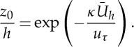
Firstly, we relate z_0,sg with the effective roughness height of the rough wall including all roughness scales starting from n=1 down to infinitely many small elements, i.e. case . Denoting z₀ as the roughness length for this surface, including all scales and for which h₁ is the largest element height, it is to be expected that z₀=C_zh₁. This scaling is expected to hold because, in the fully rough regime, the effective roughness height z₀ must scale with a characteristic roughness element height, and for a fractal surface, the only scale that can be identified is the largest scale (the large-scale cut-off). As a result of scale invariance, therefore, for an LES that resolves roughness elements only down to the nth generation, it follows that the effective roughness height of the unresolved roughness is

2.1

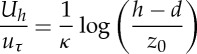
The overall roughness length z₀ can be measured dynamically in LES by invoking the log law at some height z=h:

2.2

Here is the averaged velocity at z=h, u_τ is the friction velocity, , where is the time-averaged total horizontal drag force on a planform area A_T, and ρ is the fluid density. Both and can be measured during LES. D consists of the form drag and the stress from the wall model. The form drag is obtained by integrating the pressure on the roughness elements (see [46] for a detailed description of how to obtain the pressure force from the immersed boundary method). To obtain the stress contribution from the wall model, the average streamwise-direction force per unit area applied by the integral wall model (iWMLES) is integrated over the whole ground area and roughness surfaces. For LES with the DRM, the integrated stress from the wall model includes also the drag from the subgrid roughness. The sum of the x-component (streamwise component) of the form drag and the wall shear stress yields the total drag force D. To obtain time average values of and during simulation efficiently, a weighted average is evaluated as follows:

2.3

where ϕ is the quantity for which the time mean is being evaluated (in this case, D and U_h), dt is the time step used in LES, k is the current time step index and T_ϕ is the averaging time scale. We use T_Uh,D=δ₀/(κ⋅0.1U₀) [47] for both force and velocity averaging.

Once and are determined, the DRM consists of simply rescaling the roughness length accordingly:

2.4

z_0,sg can be imposed through any LES wall closure. In the present LES, we impose it via the integral wall model [47]. Note that this DRM does not account for the displacement height, for simplicity.

In §2a, four rough-wall cases with up to four generations (g1,g2,g3,g4) are generated. Each generation resolves part of the roughness spectrum. The unresolved roughness can be modelled using the DRM (equation (2.4)). That is to say, 16 LES cases previously considered in the last section are here repeated but with the DRM implemented as part of the simulation. For cases g1, only the first generation is explicitly resolved, while all successive generations are parametrized with the DRM.

Figure 9 shows the resulting mean velocity profiles. Each profile is averaged over four realizations, i.e. over cases gn-1,2,3,4 (fixed n). We see that the profiles above h₁ are rather independent of the range of scales resolved in the LES. In table 2, we have listed all relevant quantities obtained from the LES in conjunction with the DRM. It can be observed that now z₀ is significantly larger than what was obtained with a sparse distribution of only a few generations (1–4) of roughness elements. We conclude that the DRM is able to represent self-consistently the effects of a large range of unresolved roughness elements. By rescaling the measured total drag that at each time step includes the previously evaluated and rescaled total drag force, we are effectively representing the effects of an infinitely long range of scales, nominally for .

Figure 9.

Mean velocity profiles for all cases with the DRM, in semi-log scale. Each profile is averaged among four realizations, cases gn-1,2,3,4. The inlet boundary layer height and the free stream velocity are used for normalization. (Online version in colour.)

Table 2.

A list of the relevant quantities including the effective roughness height z₀, the zero-plane displacement height d, the friction velocity u_τ and the velocity at the height of roughness layer U_h for all LES with the DRM. The height of the roughness layer (h=h₁) and the free stream velocity are used for normalization.

	g1-1	g1-2	g1-3	g1-4	g2-1	g2-2	g2-3	g2-4
Uh/U0	5.7×10−1	5.8×10−1	5.8×10−1	5.9×10−1	6.0×10−1	5.8×10−1	5.8×10−1	5.8×10−1
uτ/U0	1.0×10−1	1.0×10−1	1.1×10−1	1.0×10−1	1.1×10−1	1.0×10−1	9.8×10−2	1.1×10−1
z0/h	9.5×10−2	9.2×10−2	9.9×10−2	9.1×10−2	9.6×10−2	9.2×10−2	7.8×10−2	1.0×10−1
d/h	1.9×10−1	1.9×10−1	1.9×10−1	1.9×10−1	1.9×10−1	1.9×10−1	1.9×10−1	1.9×10−1

	g3-1	g3-2	g3-3	g3-4	g4-1	g4-2	g4-3	g4-4
Uh/U0	6.0×10−1	5.7×10−1	6.0×10−1	5.8×10−1	5.8×10−1	5.9×10−1	5.9×10−1	6.0×10−1
uτ/U0	9.8×10−2	1.1×10−1	9.7×10−2	1.0×10−1	1.0×10−1	1.0×10−1	1.0×10−1	1.1×10−1
z0/h	7.8×10−2	9.9×10−3	7.3×10−3	9.1×10−2	9.4×10−2	9.3×10−2	9.1×10−2	8.7×10−2
d/h	1.9×10−1	1.9×10−1	1.9×10−1	1.9×10−1	1.9×10−1	1.9×10−1	1.9×10−1	1.9×10−1

3. Analytical roughness for multiscale roughness

In this section, flow interactions with fractal-like roughness element distributions are modelled by adapting a new analytical approach that has been recently proposed for single-scale rectangular-prism roughness elements [17].

(a). Flow sheltering

Different from the cases considered in [17], here the major effect we need to account for is the sheltering of small-scale roughness elements by large-scale roughness elements. Flow sheltering is common in rough-wall boundary layers. Qualitatively, extreme cases are referred to as ‘d-type’ and ‘k-type’ roughness [6]. ‘d-type’ roughness elements shelter each other and the flow ‘skims’ over the roughness elements, resulting in less drag. Considerable less flow sheltering happens in ‘k-type’ roughness and each element produces almost as much drag as an isolated element. The sheltering effect among roughness elements of similar sizes has been extensively discussed (see e.g. [17,58]). The flow sheltering considered here is among roughness elements of different sizes.

Consider the flow sketched in figure 10. Downstream of a roughness element R_n, there is a reduced-momentum fluid region. It ‘shades’ the ground area beneath. The small-scale roughness elements on the shaded ground see an incoming flow with much reduced momentum and do not produce much drag. Because all roughness elements are uniformly, randomly added onto the ground, on average the number of unshaded roughness elements to all roughness elements of a particular generation n is A⁽ⁿ⁾_T,e/A_T, where A⁽ⁿ⁾_T,e is the unshaded ground area (or the ‘effective’ ground area) available for roughness R_n and A_T is the total planform area.

Figure 10.

Sheltering of small-scale roughness elements of size R_n+1 by larger-scale roughness R_n. The shaded region is the region with fluid of reduced momentum. U⁽ⁿ⁾_c is the convective velocity in the region above the sheltered region behind elements of generation n, and U⁽ⁿ⁾_t is the velocity scale of turbulent mixing.

In order to estimate the effective ground area available for roughness elements of each generation, we first need an estimate of the amount of shading one roughness element can produce. The volume of the sheltering region reduces due to vertical turbulent mixing as the fluid is convected downstream. With a convective velocity U⁽ⁿ⁾_c and a velocity scale u⁽ⁿ⁾_t for turbulent mixing, the fetch L_n it takes for the low-momentum region to be ‘eaten up’ can be approximated as (equating the streamwise travel time L_n/U⁽ⁿ⁾_c to the available transverse displacement time h_n/u⁽ⁿ⁾_t). Therefore, the ground area shaded by one roughness element R_n is approximately h_nw_nU⁽ⁿ⁾_c/u⁽ⁿ⁾_t, where w_n is the width of the roughness element. It follows that the ground area shaded by all roughness elements of the nth generation is approximately , where N_n,e is the number of R_n that are not sheltered by larger-scale roughness elements (those roughness elements that can produce significant sheltering, but for those shaded elements, they do not produce much drag nor much sheltering). Those unsheltered roughness elements R_n produce shades that further reduce the effective ground area available for roughness elements of the next generation (figure 11).

Figure 11.

Modelled flow interactions with ground roughness. Large-scale roughness shades the small-scale roughness. Unshaded small-scale roughness further shades the lesser-scale roughness elements.

We can now define the frontal area of the unsheltered elements of roughness elements of the nth generation to be the ‘effective frontal area’ A⁽ⁿ⁾_f,e=N_n,eh_nw_n. This is the frontal area that is directly associated with pressure drag force. The ‘effective’ ground area that is left for the next generation is

3.1

λ_p,n is constant (with respect to n) for the roughness considered in §2. Placing roughness elements of the nth generation R_n takes planform area, leading to the first term on the right-hand side of equation (3.1). The second term is due to sheltering. The effective frontal area at the nth generation is (on average) determined by the effective ground area available for the nth generation, and is given by

3.2

again is a constant (with respect to n) for the ground roughness considered in §2.

Equations (3.1) and (3.2) are the recurrence relations for calculating the effective ground area and effective frontal area at each generation. For n=1, A⁽¹⁾_T,e is the nominal total ground area and A⁽¹⁾_f,e is the nominal frontal area of the roughness of the first generation. In this discussion, we have neglected the flow sheltering among roughness elements of the same size as well as the sheltering of large-scale roughness by small-scale roughness. The latter effect is presumably not significant. Neglecting the former effect, however, restricts the application of this model to small λ⁽ⁿ⁾_f, where sheltering among roughness elements of the same size is weak. A correction can be made to account for this effect, and it is discussed later in this section.

We still need to estimate . It is not unreasonable to assume that the flow, by interacting with scale-invariant ground roughness, becomes scale-invariant. Scale invariance and self-similarity in the flow indicate that the ratio should be independent of n. We denote this constant as α and evaluate α at a particular scale, namely n=1. At the first generation, the mean velocity at z=h₁ can be used as the convective velocity and the velocity scale for turbulent mixing is simply the friction velocity u_τ. Therefore, we have

3.3

We now solve for A⁽ⁿ⁾_T,e and A⁽ⁿ⁾_f,e using the recurrence relations in equations (3.1) and (3.2). Substituting equation (3.3) into equation (3.1) leads to

3.4

which in turn leads to

3.5

A⁽ⁿ⁾_f,e can then be determined using the equation:

3.6

For the ground roughness considered in §2, λ_f=0.014, λ_p=0.056. However, an estimate for is still required.

(b). Constraints from conservation laws

In this subsection, fundamental constraints from conservation laws (momentum and velocity continuity) are incorporated in order to derive an estimate of α. First, we use the momentum balance to argue that the drag from the ground roughness elements is balanced by the downward momentum flux:

3.7

Above, N is the number of roughness generations, C_dh is the drag coefficient for an isolated rectangular roughness defined based on the top velocity and we have used the quadratic law for the drag. Velocity continuity at the top of the boundary layer and at z=h (where we are setting h=h₁) imposes two constraints:

3.8

and

3.9

where U₀ is the free stream velocity, Π is the strength of the wake function [59] and is typically of order unity [6], δ is the boundary layer height, d is the displacement height, z₀ is the effective roughness height and κ=0.4 is the von Karman constant. Last, we invoke the hypothesis that d is the centroid height of the distributed drag force [57]:

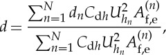3.10

where d_n is the centroid height of the drag force associated with the roughness of the nth generation.

Equations (3.7)–(3.10) can be used to solve for u_τ, U_h, z₀ and d. Define β_n=U(z=h_n)/U_h and γ_n=d_n/h_n. Equation (3.7) leads to

3.11

Rewriting equation (3.10) using β_n=U(z=h_n)/U_h and γ_n=d_n/h_n gives

3.12

Substituting equation (3.10) into equation (3.8) leads to

3.13

u_τ can be calculated using equation (3.9):

3.14

and U_h is

3.15

The effective frontal area is given by equation (3.5). With β_n and d_n known, equations (3.11)–(3.15) can be successively used to get α, d, z₀, u_τ and U_h.

However, β_n and γ_n still need to be estimated.

(c). Flow in the near-wall region

In this subsection, we estimate β_n and γ_n by examining the flow in the near-wall region. The mean flow in the near-wall region is known to be approximated well by exponential behaviour [17,60,61]:

3.16

where U_h is the velocity at the top of the roughness layer, h is the roughness layer height and a is the so-called ‘attenuation coefficient’. The overall shape of the exponential is controlled by this attenuation factor.

Also, d_n is the centroid of the drag force associated with the roughness of the nth generation. Because of self-similarity and scale invariance in the flow, it is reasonable to assume that γ_n=d_n/h_n is a constant (with respect to n). Therefore,

3.17

where C_d is the sectional drag coefficient. Roughness elements that contribute to the momentum balance and subsequently to equation (3.10) are unsheltered elements and produce as much drag as isolated elements. Therefore, in equation (3.17), the attenuation coefficient for a sheltered roughness element, a₀, needs to be used.

Equating the drag force over an isolated roughness element to the distributed canopy drag force generated by the average profile yields

3.18

Substituting equation (3.16) into equation (3.18), the attenuation coefficient for an unsheltered rectangular roughness element can be solved for. Using typically measured values for C_d=1 [15] and C_dh=0.7 [62–64], the attenuation factor for an isolated roughness element is a₀≈0.4, as shown in [17]. Substituting into equation (3.17) leads to

3.19

For an estimate of β_n, we use equation (3.16) with a=a₀:

3.20

Using h_n=h/2ⁿ⁻¹, equation (3.20) leads to

3.21

(d). Sheltering among roughness elements of the same size

So far we have neglected the sheltering among roughness elements of the same size. We can include this effect by considering the probability that a roughness element that is not sheltered by larger-size roughness elements is sheltered by an element of its same size. The corrected, reduced, effective frontal area A′_f,e is written as

3.22

where p_n is the probability that a roughness of scale R_n is not in the shade of R_n′ elements (where n′<n) nor in the shade of any roughness elements of scale R_n:

3.23

As expected from scale invariance, this probability remains a constant independent of n.

(e). Results

The analytical model is given by equations (3.6), (3.11)–(3.15), (3.19) and (3.21) (and equation (3.22) when including same-scale sheltering). Predictions of the analytical model include values of z₀, d, u_τ (and therefore the drag force) and U_h. The inputs required by the model include knowledge about the element's shape and density distribution, the number of generations captured (in the analytical model this is denoted by N), the boundary layer height δ and the free stream velocity U₀. The parameters used in this model include the von Karman constant for which a standard value κ=0.4 is here taken, the sectional drag coefficient C_d=1, drag coefficient defined based on the top velocity C_dh=0.7 and the strength of the wake function, for which we use Π=0.1 (for a mild wake function).

The analytical model is algebraic so that no differential equation solution or numerical integration is required, although because of the coupling in equations (3.6) and (3.11), the system needs to be solved iteratively, and therefore numerically (because of the exponential including a power, the sum in equation (3.6) is not a simple geometric sum). Equations (3.6) and (3.11) should be solved iteratively for α and A⁽ⁿ⁾_f,e. Once these are known, equations (3.12)–(3.15) can be sequentially used to solve for d, z₀, u_τ and U_h.

Figures 12a–d compare the model predictions against the measurements from LES with and without the DRM. In figure 12a we see that the model (solid line) accurately follows the initial increase in z₀ observed earlier in the LES without the DRM (for which n=N, as in LES without DRM the cases for generation n contained only up to n elements without additional SGS contributions). Once the DRM approach is implemented in LES, one may consider that the LES is simulating the asymptotic case with infinitely many SGS roughness elements, due to the recursive renormalization inherent in the DRM approach. The resulting z₀ is much larger, around 0.09h₁, and is plotted here at generation number N=25 as it appears that by then the trend has converged and the drag is not further increasing. Naturally, in physical scales, N=25 is unrealistic as by then the SGS elements would be far below the viscous range. Still the DRM in this case assumes arbitrarily high Reynolds number and so does the analytical model, so the comparison is still a fair one. Clearly, neglecting the sheltering effect (dashed line) yields slightly less accurate trends.

Figure 12.

A comparison of analytical model predictions and LES measurements. Symbols at N=25 are from LES with the dynamic model. The solid lines are predictions that include sheltering among roughness elements of the same size using equation (3.22) while the dashed lines are predictions without this correction. The symbols are LES measurements. For g1, g2, g3 and g4, the unresolved roughness is not included (no roughness wall model). Results shown are averaged among four LES runs gn-1,2,3,4. For g25, the average is among 16 LES. The error bar (the size of one leg) indicates the largest deviation from the mean in the LES measurements.

The model yields the displacement height as shown in figure 12b. As discussed before, this quantity is not measured from the LES but only modelled so no comparison can be made. The predictions of the friction velocity (drag) in figure 12c are rather excellent across all generations. The velocity at roughness height z=h₁ also agrees reasonably well with the model, as seen in figure 12d.

4. Conclusion

We conduct LES of turbulent boundary layers over random distributions of rectangular-prism roughness elements with a fractal-like, discrete, size distribution. First we consider finite hierarchies of scales. The flow response to the range of scales in ground roughness is investigated by successively adding roughness generations of decreasing scales on the bottom surface of the computational domain. A DRM is then developed to model the drag from unresolved roughness elements. The DRM assumes that the flow, by interacting with the self-invariant roughness element distribution, becomes itself scale-invariant. LES with this DRM yields mean flow profiles that show little or no dependence on the range of scales resolved in the simulation (grid resolution), allowing us to conclude that the DRM model is successful at reproducing the effects of SGS roughness elements regardless of how many generations are kept in the numerically resolved, and in the SGS, ranges, respectively.

Moreover, the flow interactions with fractal-like ground roughness are modelled using a fully analytical model that includes explicit accounting of sheltering and basic considerations of momentum balance and velocity continuity. It also includes a few required parameters such as the drag coefficient of individual rectangular-prism elements and the von Karman constant. Predictions from this analytical model depend explicitly on the number of generations included in the roughness. Thus, results could be compared with the LES at various resolutions, as well as with the DRM-based LES for the case that aims at representing the situation including a very large number of generations or roughness elements. Good agreement between the analytical model and LES results is found.

Limitations of the present study are that only rectangular-prism elements have so far been considered, and of a single aspect ratio. Also, only the limit of fully rough surfaces was considered here, in which no Reynolds-number dependences could be captured. Clearly further studies are needed to expand the formalism to more general geometries and Reynolds numbers. Ultimately, it is hoped that such models may help in the context of analytical wind farm models and LES of wind farms in complex terrain.

Authors' contributions

X.I.A.Y. carried out the simulations. C.M. and X.I.A.Y. jointly developed the dynamic roughness model, analysed the results, developed the analytical roughness model and wrote, read and approved the manuscript.

Competing interests

We declare we have no competing interests.

Funding

The authors thank the ONR and NSF (AGS-1045189) for financial support.

References

- 1.Palma J, Castro F, Ribeiro L, Rodrigues A, Pinto A. 2008. Linear and nonlinear models in wind resource assessment and wind turbine micro-siting in complex terrain. J. Wind Eng. Ind. Aerodyn. 96, 2308–2326. ( 10.1016/j.jweia.2008.03.012) [DOI] [Google Scholar]
- 2.Uchida T, Ohya Y. 2008. Micro-siting technique for wind turbine generators by using large-eddy simulation. J. Wind Eng. Ind. Aerodyn. 96, 2121–2138. ( 10.1016/j.jweia.2008.02.047) [DOI] [Google Scholar]
- 3.Politis ES, Prospathopoulos J, Cabezon D, Hansen KS, Chaviaropoulos P, Barthelmie RJ. 2012. Modeling wake effects in large wind farms in complex terrain: the problem, the methods and the issues. Wind Energy 15, 161–182. ( 10.1002/we.481) [DOI] [Google Scholar]
- 4.Santoni C, Ciri U, Leonardi S. 2015. Effect of topography on wind turbine power and load fluctuations. Bull. Am. Phys. Soc. 60, abstract L12.002. [Google Scholar]
- 5.Raupach M, Antonia R, Rajagopalan S. 1991. Rough-wall turbulent boundary layers. Appl. Mech. Rev. 44, 1–25. ( 10.1115/1.3119492) [DOI] [Google Scholar]
- 6.Jiménez J. 2004. Turbulent flows over rough walls. Annu. Rev. Fluid Mech. 36, 173–196. ( 10.1146/annurev.fluid.36.050802.122103) [DOI] [Google Scholar]
- 7.Castro IP. 2007. Rough-wall boundary layers: mean flow universality. J. Fluid Mech. 585,469–485. ( 10.1017/S0022112007006921) [DOI] [Google Scholar]
- 8.Castro IP. 2009. Turbulent flow over rough walls. In Advances in turbulence XII, pp. 381–388. Berlin, Germany: Springer.
- 9.Flack KA, Schultz MP. 2010. Review of hydraulic roughness scales in the fully rough regime. J. Fluids Eng. 132, 041203 ( 10.1115/1.4001492) [DOI] [Google Scholar]
- 10.Cheng H, Castro IP. 2002. Near wall flow over urban-like roughness. Bound.-Layer Meteorol. 104, 229–259. ( 10.1023/A:1016060103448) [DOI] [Google Scholar]
- 11.Castro IP, Cheng H, Reynolds R. 2006. Turbulence over urban-type roughness: deductions from wind-tunnel measurements. Bound.-Layer Meteorol. 118, 109–131. ( 10.1007/s10546-005-5747-7) [DOI] [Google Scholar]
- 12.Xie Z, Castro IP. 2006. LES and RANS for turbulent flow over arrays of wall-mounted obstacles. Flow Turbul. Combust. 76, 291–312. ( 10.1007/s10494-006-9018-6) [DOI] [Google Scholar]
- 13.Cheng WC, Porté-Agel F. 2015. Adjustment of turbulent boundary-layer flow to idealized urban surfaces: a large-eddy simulation study. Bound.-Layer Meteorol. 155, 249–270. ( 10.1007/s10546-015-0004-1) [DOI] [Google Scholar]
- 14.Grimmond C, Oke TR. 1999. Aerodynamic properties of urban areas derived from analysis of surface form. J. Appl. Meteorol. 38, 1262–1292. ( 10.1175/1520-0450(1999)038%3C1262:APOUAD%3E2.0.CO;2) [DOI] [Google Scholar]
- 15.Coceal O, Belcher S. 2004. A canopy model of mean winds through urban areas. Q. J. R. Meteorol. Soc. 130, 1349–1372. ( 10.1256/qj.03.40) [DOI] [Google Scholar]
- 16.Di Sabatino S, Solazzo E, Paradisi P, Britter R. 2008. A simple model for spatially-averaged wind profiles within and above an urban canopy. Bound.-Layer Meteorol. 127, 131–151. ( 10.1007/s10546-007-9250-1) [DOI] [Google Scholar]
- 17.Yang XIA, Sadique J, Mittal R, Meneveau C. 2016. Exponential roughness layer and analytical model for turbulent boundary layer flow over rectangular-prism roughness elements. J. Fluid Mech. 789, 127–165. ( 10.1017/jfm.2015.687) [DOI] [Google Scholar]
- 18.Yang XIA. 2016. On the mean flow behaviour in the presence of regional-scale surface roughness heterogeneity. Bound.-Layer Meteorol. 161, 127–143. ( 10.1007/s10546-016-0154-9) [DOI] [Google Scholar]
- 19.Schultz MP, Flack KA. 2009. Turbulent boundary layers on a systematically varied rough wall. Phys. Fluids 21, 015104 ( 10.1063/1.3059630) [DOI] [Google Scholar]
- 20.Bhaganagar K, Kim J, Coleman G. 2004. Effect of roughness on wall-bounded turbulence. Flow Turbul. Combust. 72, 463–492. ( 10.1023/B:APPL.0000044407.34121.64) [DOI] [Google Scholar]
- 21.Brown AR, Hobson J, Wood N. 2001. Large-eddy simulation of neutral turbulent flow over rough sinusoidal ridges. Bound.-Layer Meteorol. 98, 411–441. ( 10.1023/A:1018703209408) [DOI] [Google Scholar]
- 22.Nikuradse J. 1950. Laws of flow in rough pipes. Washington, DC: National Advisory Committee for Aeronautics. [Google Scholar]
- 23.Schultz M, Flack K. 2005. Outer layer similarity in fully rough turbulent boundary layers. Exp. Fluids 38, 328–340. ( 10.1007/s00348-004-0903-2) [DOI] [Google Scholar]
- 24.Schultz M, Flack K. 2007. The rough-wall turbulent boundary layer from the hydraulically smooth to the fully rough regime. J. Fluid Mech. 580, 381–405. ( 10.1017/S0022112007005502) [DOI] [Google Scholar]
- 25.Rodriguez-Iturbe I, Marani M, Rigon R, Rinaldo A. 1994. Self-organized river basin landscapes: fractal and multifractal characteristics. Water Resour. Res. 30, 3531–3539. ( 10.1029/94WR01493) [DOI] [Google Scholar]
- 26.Rodríguez-Iturbe I, Rinaldo A. 2001. Fractal river basins: chance and self-organization. Cambridge, UK: Cambridge University Press. [Google Scholar]
- 27.Mazzi B, Vassilicos J. 2004. Fractal-generated turbulence. J. Fluid Mech. 502, 65–87. ( 10.1017/S0022112003007249) [DOI] [Google Scholar]
- 28.Nicolleau F, Salim S, Nowakowski A. 2011. Experimental study of a turbulent pipe flow through a fractal plate. J. Turbul. 12, N44 ( 10.1080/14685248.2011.637046) [DOI] [Google Scholar]
- 29.Seoud R, Vassilicos J. 2007. Dissipation and decay of fractal-generated turbulence. Phys. Fluids 19, 105108 ( 10.1063/1.2795211) [DOI] [Google Scholar]
- 30.Staicu A, Mazzi B, Vassilicos J, van de Water W. 2003. Turbulent wakes of fractal objects. Phys. Rev. E 67, 066306 ( 10.1103/PhysRevE.67.066306) [DOI] [PubMed] [Google Scholar]
- 31.Hurst D, Vassilicos J. 2007. Scalings and decay of fractal-generated turbulence. Phys. Fluids 19, 035103 ( 10.1063/1.2676448) [DOI] [Google Scholar]
- 32.Bai K, Meneveau C, Katz J. 2012. Near-wake turbulent flow structure and mixing length downstream of a fractal tree. Bound.-Layer Meteorol. 143, 285–308. ( 10.1007/s10546-012-9700-2) [DOI] [Google Scholar]
- 33.Bai K, Meneveau C, Katz J. 2013. Experimental study of spectral energy fluxes in turbulence generated by a fractal, tree-like object. Phys. Fluids 25, 110810 ( 10.1063/1.4819351) [DOI] [Google Scholar]
- 34.Bai K, Katz J, Meneveau C. 2015. Turbulent flow structure inside a canopy with complex multi-scale elements. Bound.-Layer Meteorol. 155, 435–457. ( 10.1007/s10546-015-0011-2) [DOI] [Google Scholar]
- 35.Chester S, Meneveau C, Parlange MB. 2007. Modeling turbulent flow over fractal trees with renormalized numerical simulation. J. Comput. Phys. 225, 427–448. ( 10.1016/j.jcp.2006.12.009) [DOI] [Google Scholar]
- 36.Chester S, Meneveau C. 2007. Renormalized numerical simulation of flow over planar and non-planar fractal trees. Environ. Fluid Mech. 7, 289–301. ( 10.1007/s10652-007-9026-7) [DOI] [Google Scholar]
- 37.Graham J, Meneveau C. 2012. Modeling turbulent flow over fractal trees using renormalized numerical simulation: alternate formulations and numerical experiments. Phys. Fluids 24, 125105 ( 10.1063/1.4772074) [DOI] [Google Scholar]
- 38.Anderson W, Meneveau C. 2011. Dynamic roughness model for large-eddy simulation of turbulent flow over multiscale, fractal-like rough surfaces. J. Fluid Mech. 679, 288–314. ( 10.1017/jfm.2011.137) [DOI] [Google Scholar]
- 39.Anderson W, Passalacqua P, Porté-Agel F, Meneveau C. 2012. Large-eddy simulation of atmospheric boundary-layer flow over fluvial-like landscapes using a dynamic roughness model. Bound.-Layer Meteorol. 144, 263–286. ( 10.1007/s10546-012-9722-9) [DOI] [Google Scholar]
- 40.Frandsen S, Barthelmie R, Pryor S, Rathmann O, Larsen S, Hojstrup J, Thogersen M. 2006. Analytical modelling of wind speed deficit in large offshore wind farms. Wind. Energy 9, 39–53. ( 10.1002/we.189) [DOI] [Google Scholar]
- 41.Calaf M, Meneveau C, Meyers J. 2010. Large eddy simulation study of fully developed wind-turbine array boundary layers. Phys. Fluids 22, 015110 ( 10.1063/1.3291077) [DOI] [Google Scholar]
- 42.Meneveau C. 2012. The top-down model of wind farm boundary layers and its applications. J. Turbul. 13, N7 ( 10.1080/14685248.2012.663092) [DOI] [Google Scholar]
- 43.Raupach M. 1992. Drag and drag partition on rough surfaces. Bound.-Layer Meteorol. 60, 375–395. ( 10.1007/BF00155203) [DOI] [Google Scholar]
- 44.Shao Y, Yang Y. 2005. A scheme for drag partition over rough surfaces. Atmos. Environ. 39, 7351–7361. ( 10.1016/j.atmosenv.2005.09.014) [DOI] [Google Scholar]
- 45.Shao Y, Yang Y. 2008. A theory for drag partition over rough surfaces. J. Geophys. Res. 113, F02S05 ( 10.1029/2007JF000791) [DOI] [Google Scholar]
- 46.Mittal R, Dong H, Bozkurttas M, Najjar F, Vargas A, von Loebbecke A. 2008. A versatile sharp interface immersed boundary method for incompressible flows with complex boundaries. J. Comput. Phys. 227, 4825–4852. ( 10.1016/j.jcp.2008.01.028) [DOI] [PMC free article] [PubMed] [Google Scholar]
- 47.Yang XIA, Sadique J, Mittal R, Meneveau C. 2015. Integral wall model for large eddy simulations of wall-bounded turbulent flows. Phys. Fluids 27, 025112 ( 10.1063/1.4908072) [DOI] [Google Scholar]
- 48.Yang XIA, Meneveau C. 2016. Recycling inflow method for simulations of spatially evolving turbulent boundary layers over rough surfaces. J. Turbul. 17, 75–93. ( 10.1080/14685248.2015.1090575) [DOI] [Google Scholar]
- 49.Yang XIA, Sadique J, Meneveau C, Mittal R. 2015. Applications of the integral wall model in LES of flow over surfaces including resolved and subgrid roughness. In 22nd AIAA Computational Fluid Dynamics Conference, Dallas, TX ( 10.2514/6.2015-2919) [DOI]
- 50.Vedula V, Fortini S, Seo J, Querzoli G, Mittal R. 2014. Computational modeling and validation of intraventricular flow in a simple model of the left ventricle. Theor. Comput. Fluid Dyn. 28, 589–604. ( 10.1007/s00162-014-0335-4) [DOI] [Google Scholar]
- 51.Bhardwaj R, Mittal R. 2012. Benchmarking a coupled immersed-boundary–finite-element solver for large-scale flow-induced deformation. AIAA J. 50, 1638–1642. ( 10.2514/1.J051621) [DOI] [Google Scholar]
- 52.Zheng L, Hedrick TL, Mittal R. 2013. A multi-fidelity modelling approach for evaluation and optimization of wing stroke aerodynamics in flapping flight. J. Fluid Mech. 721, 118–154. ( 10.1017/jfm.2013.46) [DOI] [Google Scholar]
- 53.Meinders E, Hanjalić K. 1999. Vortex structure and heat transfer in turbulent flow over a wall-mounted matrix of cubes. Int. J. Heat Fluid Flow 20, 255–267. ( 10.1016/S0142-727X(99)00016-8) [DOI] [Google Scholar]
- 54.Graham J. et al. 2016. A web services accessible database of turbulent channel flow and its use for testing a new integral wall model for LES. J. Turbul. 17, 181–215. ( 10.1080/14685248.2015.1088656) [DOI] [Google Scholar]
- 55.Piomelli U. 2008. Wall-layer models for large-eddy simulations. Progr. Aerosp. Sci. 44, 437–446. ( 10.1016/j.paerosci.2008.06.001) [DOI] [Google Scholar]
- 56.Larsson J, Kawai S, Bodart J, Bermejo-Moreno I. 2016. Large eddy simulation with modeled wall-stress: recent progress and future directions. Mech. Eng. Rev. 3, 15-00418 ( 10.1299/mer.15-00418) [DOI] [Google Scholar]
- 57.Jackson P. 1981. On the displacement height in the logarithmic velocity profile. J. Fluid Mech. 111, 15–25. ( 10.1017/S0022112081002279) [DOI] [Google Scholar]
- 58.Leonardi S, Orlandi P, Antonia R. 2007. Properties of d- and k-type roughness in a turbulent channel flow. Phys. Fluids 19, 125101 ( 10.1063/1.2821908) [DOI] [Google Scholar]
- 59.Coles D. 1956. The law of the wake in the turbulent boundary layer. J. Fluid Mech. 1, 191–226. ( 10.1017/S0022112056000135) [DOI] [Google Scholar]
- 60.Cionco RM. 1965. A mathematical model for air flow in a vegetative canopy. J. Appl. Meteorol. 4, 517–522. ( 10.1175/1520-0450(1965)004%3C0517:AMMFAF%3E2.0.CO;2) [DOI] [Google Scholar]
- 61.Macdonald R, Griffiths R, Hall D. 1998. An improved method for the estimation of surface roughness of obstacle arrays. Atmos. Environ. 32, 1857–1864. ( 10.1016/S1352-2310(97)00403-2) [DOI] [Google Scholar]
- 62.Akins RE, Peterka JA, Cermak JE. 1977. Mean force and moment coefficients for buildings in turbulent boundary layers. J. Wind Eng. Ind. Aerodyn. 2, 195–209. ( 10.1016/0167-6105(77)90022-8) [DOI] [Google Scholar]
- 63.Curley A, Uddin M, Peters B. 2015. Direct numerical simulation of turbulent flow around a surface mounted cube. In 22nd AIAA Computational Fluid Dynamics Conference, paper 3431.
- 64.Hussain M, Lee B. 1980. A wind tunnel study of the mean pressure forces acting on large groups of low-rise buildings. J. Wind Eng. Ind. Aerodyn. 6, 207–225. ( 10.1016/0167-6105(80)90002-1) [DOI] [Google Scholar]