The organization of orientation and spatial frequency in primary visual cortex

Abstract

Many studies have demonstrated that the primary visual cortex contains multiple functional maps of visual properties (e.g., ocular dominance, orientation preference, and spatial-frequency preference), but as yet no consistent picture has emerged as to how these maps are related to one another. Three divergent, prior optical-imaging studies of spatial frequency are reanalyzed and critiqued in this article. Evidence is presented that a nonstimulus-specific response biased the interpretation of results in previous studies. In addition to reexamining four prior cat experiments, we carried out one new experiment. Through the use of different methods and a careful removal of the nonspecific response, we are led in all instances to a unique view of cortical organization for spatial-frequency preference. In particular, we find little apparent evidence for a columnar organization for spatial frequency. The response recorded by each image pixel may be viewed as arising from an admixture of low- and high-spatial-frequency populations. For most pixels, the ratio of these populations is 1:1.

The retinotopic map relates an element of visual space to an element of cortical tissue. Neurons in the primary visual cortex are known to be differentially sensitive to orientation, θ, and spatial frequency (SF), k, of corresponding image elements that appear in visual space.‡ Thus, it may be said that the primary visual cortex maps visual space through a local Fourier analysis (1, 2). The process by which this mapping takes place, although not fully understood, is known to involve information processing by the retina, lateral geniculate nucleus (LGN), and primary visual cortex area V1 (V1) and feedback from higher areas.

Casting aside the nature of neuronal circuitry, the functional layout of the primary visual cortex is well established for orientation preference and ocular dominance. Anatomical (3–5) and optical-imaging (6–9) studies have elaborated and extended the columnar view of V1 that emerged from electrophysiology (10, 11). Less can be said of the representation of SF. Extensive electrophysiological recordings (12–17) and optical-imaging experiments have not provided a consistent picture of SF layout. The situation can be further complicated if variations in the temporal properties of the stimuli are included (18).

One series of optical-imaging studies (7, 19–22) advanced the viewpoint that the orientation layout of V1 is organized into high- and low-SF preference columns. From this view, it follows that only a single map is needed to characterize SF. This map contains regions corresponding to high and low SF with opposite signs. Thus high- and low-SF stimuli result in responses of opposite signatures. An obvious shortcoming is that intermediate SF would lead to null or near-null results. On the other hand, Everson et al. (23) reported that SF preference is continuously distributed and that at least two maps are required to depict SF representation in the primary visual cortex. More recently, Issa et al. (24), while confirming that SF is continuously distributed, suggested that the pinwheel centers of the orientation layout alternate as loci for columns of relatively high- and low-SF preference. On this basis, Bressloff, Cowan, and colleagues (25) proposed a spherical model of orientation and SF, with orientation as the azimuthal variable and low and high SF in the polar regions. The earlier representation of De Valois and De Valois (17) suggests another geometric model for k and θ, namely an infinite cylinder in which ln k is the axial coordinate. Additionally, based on 2-deoxyglucose studies, De Valois and De Valois (17) suggest that CO blobs are loci of low-SF preference as well as pinwheel centers. The De Valois model also serves as a test-bed for the analysis presented below. (For additional information, see Supporting Appendix and Figs. 6–13, which are published as supporting information on the PNAS web site.)

It is our contention that the analysis used in previous optical-imaging studies was compromised by the “nonspecific response,” a blood-related artifact. This term (discussed below) refers to “a response evoked by the stimulus but which does not depend on the specific nature of the stimulus” (26). Here we demonstrate that, if the nonspecific response is removed, a different conceptual model of the functional architecture emerges.

In this article we (i) implement an objective method for the removal of the nonspecific response; (ii) apply a powerful new feature for analyzing optical images; and (iii) show that there is little evidence for SF columns on the scale of cortical orientation columns.

Methods

Experimental procedures were approved by the Mount Sinai School of Medicine Institutional Animal Care and Use Committee and were performed in compliance with guidelines established by the National Institutes of Health (Bethesda).

We report on experiments carried out on five adult cats. Details of the surgery and imaging are presented in Everson et al. (23) and Issa et al. (24). Previously reported data sets (four cats) have been reexamined. Specific details and results are contained in the text and in the supporting information. For purposes of this article, one further experiment was conducted to verify the new conclusions. For this experiment, surgery and imaging differed from the previous studies as described in the following sections.

Surgery. Anesthesia was maintained with i.v. infusion of a mixture of propofol (4 mg/kg per hr; Diprivan, AstraZeneca) and sufentanil (0.05 μg/kg per hr). The cranial chamber was filled with liquid silicone polymer (Klarisil-H, Dreve Otoplastik, Unna, Germany).

Visual Stimuli. Full-field stimuli consisted of drifting sinusoidal gratings presented binocularly at six orientations (0°, 30°, 60°, 90°, 120°, and 150°) and seven SFs [0.035, 0.07, 0.14, 0.28, 0.56, 1.12, and 2.24 cycles per degree (c/deg)]. The gratings drifted at 2 Hz and were of 100% contrast.

Image Analysis. In optical imaging, the background signal, because of diverse causes, confers an extremely small signal-to-noise ratio, O(10^-3), on the image data (26). For example, respiration and circulation are huge background sources of noise. All methods for extracting response maps from such images rely on some form of subtracting out the unwanted background signal, sometimes in a disguised form. A problematical noise source, termed the nonspecific response, is a component of the response that does not depend on the specific nature of the stimulus. To describe the origin of the nonspecific signal, we begin with the widely held view that the intrinsic signal arises largely from changes in the hemodynamic (and light-scattering) properties of cortical tissue and measures metabolic response caused by neuronal activity. In response to a stimulus, say, a drifting grating of fixed k, increased metabolic demand from neuronal activity originates in the relatively small patch of tissue that contains those neurons preferentially responding to this stimulus. However, a larger patch, the vascular bed, is mobilized to meet this metabolic demand (27, 28). Because all orientations are equally represented, one might expect roughly the same vascular bed to be active at all orientations at the same SF. This scenario leads to a picture of the response consisting of two elements: one small specific region dependent on θ and a larger region that is nonspecific to θ. Further, one should expect that the map of both regions depends on the strength of response, which in this instance implies a dependence on k. (In the experiments, contrast is fixed and does not enter.) We next present a general method for removing the nonspecific response.

Consider f = f(t, x, k, θ), a collection of intrinsic images at SF, k, and orientation, θ. f is the response, measured as a gray level at pixel location x at time t (t serves as an image index). If k is fixed, it then follows that the strength of the nonspecific response also is fixed. The response, cleansed of background and the nonspecific response, can be conveniently thought of as being given by§

[1]

The brackets, 〈 and 〉, denote an average. The difference inside the outer bracket indicates that the average over all orientations, 〈f(t, x, θ; k)〉_θ, at fixed k, is to be removed from every image. Because this process is carried out for fixed k, it serves to remove background (k follows the semicolon in Eq. 1 to emphasize that this is done at fixed SF). It also removes whatever nonspecific signal exists. The difference is then averaged over all time. The procedure contained in Eq. 1 is carried out for each k, and the assembled result is denoted by r = r(k, θ, x), in contrast with Eq. 1. A common error in dealing with SF data is the pooling of data at different SF. As discussed in more detail in Comparison with Previous Studies, this pooling leaves a residual nonspecific artifact in the results. In practice, the simple difference in Eq. 1 requires large amounts of data to be effective.

Virtually all analyses of optical imaging rely on some form of differencing, as indicated by Eq. 1. For unlimited data, Eq. 1 removes all artifacts, but limitless data are unrealistic, and a number of procedures have been proposed for accelerating the differencing process (26). A powerful method for accomplishing this outcome, based on multivariate statistics, is the GIFA procedure (29), which is briefly summarized in Supporting Appendix.

Results

We use the same notation as Eq. 1 and denote the cleansed response by r = r(k, θ, x), with r the gray level at pixel location x, due to a stimulus of SF k, at orientation θ.

The singular value decomposition (SVD) seeks a coordinate system that is intrinsic to the data and leads to an optimally concise representation of the data, an ideal framework for analysis. If applied to r(k, θ, x), it yields the series representation

[2]

The terms of the series are arranged in order of decreasing importance. The constants, , the spectrum of the decomposition, are variances that measure the energy in the corresponding components. A typical plot of μ_n is shown in Fig. 1. Orientation and SF dependence reside in the orthonormal set {a_n}, and pixel dependence is contained in the orthonormal maps {ϕ_n}.

Fig. 1.

Spectrum of coefficients, μ_n, for the expansion r = ∑_n a_n(θ, k)μ_nϕ_n(x). The μ_ns are the singular values obtained by performing an SVD on r. Variances are proportional to , and hence Eq. 3 captures ≈95% of the variance.

From Fig. 1, we see that the first two modes are dominant. A key insight is obtained by applying SVD to each a_n(k, θ). From this, we discover that a_n ≈ α_n(k)β_n(θ), where 99.5% of the variance is captured for n = 1, 99% for n = 2, 95% for n = 3, and 90% for n = 4. Thus, to relatively high accuracy, the coefficients a_n(k, θ) are factorable. Fig. 2 displays the plots of α_n(k) and β_n(θ) for n = 1,...,4.We easily see that β₁(θ) ≈ β₃(θ) and β₂(θ) ≈ β₄(θ) so that (β₁, β₂) ≈ (β₃, β₄). Further, from Fig. 2a, α₁(k) ≈ α₂(k) and α₃(k) ≈ α₄(k), i.e., the SF factors come in pairs. We can therefore write r in the form

[3]

This form captures ≈95% of the signal in r.

Fig. 2.

SF and orientation filters obtained by performing SVD on a_n(θ, k). (a) SF filters, α_n(k). Smooth curves are bicubic spline interpolations of data points (□). Note that α₁ ≈ α₂ and α₃ ≈ α₄. The green curve represents the average SF tuning curve over all pixels. (b) Orientation filters, β_n(θ). Note that β₁ and β₃ resemble cos(2θ - ϕ) and β₂ and β₄ resemble sin(2θ - ϕ).

The orientation functions β₁(θ) and β₂(θ), shown in Fig. 2, are to within 2% error, proportional to sin 2(θ - ϕ) and cos 2(θ - ϕ), where ϕ is a phase offset determined by the data. That a single harmonic, (sin 2θ, cos 2θ), dominates Eq. 3 is a consequence of the fact that, to good approximation, all orientations are represented equally on the cortex (8, 23).When equality holds, β_n is a sinusoid and separability is exact.

Because μ₅ and μ₆ are roughly the same order as μ₃ and μ₄, omission of the corresponding modes might seem arbitrary. Modes (a₅(k, θ), a₆(k, θ)) are approximately equal to α₁(k) × (β₁(2θ), β₂(2θ)), which, from above, are fourth harmonics in θ. When μ₅ and μ₆ are included in the calculation, these terms make a small correction to the first term of Eq. 3. Because orientation tuning width can be calculated from fourth harmonics, including these terms could be of value. However, in view of the noisy quality of ϕ₅(x) and ϕ₆(x), we have neglected these terms.

Coefficients of ϕ_n(x), in Eq. 3, are of product form, α_n(k)β_n(θ), and are orthonormal. The orthogonal separability of SF and orientation preference is an approximate property of a_n(k, θ) (Eq. 3). The approximate character of this feature may be traced to the lack of uniformity in orientation preference (oblique effect) and the degree to which individual neurons exhibit separability in SF and θ. This separability has been a disputed issue (30–32) with evidence on both sides (24, 33, 34). Recordings in a recent study by Mazer et al. (35) from awake behaving monkeys point toward separability, but Ringach et al. (36) arrive at a different conclusion.

Each bracketed term of Eq. 3, corresponding to the two SF factors α₁(k) and α₃(k), generates a preferred orientation map. Orientation space is covered twice by Eq. 3, i.e., each of the SF eigenfunctions has a corresponding pair of orientation eigen-functions.

A Transformation. In Fig. 2a we indicate, by the green curve, the global distribution of SF preference of the cortical region under investigation [the rms of r(k, θ, x) taken over all pixels and angles]. This curve is closely approximated by α₁(k) and also closely fits the standard cat contrast sensitivity function (17). From Eq. 3, each pixel can be regarded as an admixture of contributions from SF eigenfunctions α₁(k) and α₃(k), which reflect the distribution of underlying SF preference of the single units at that cortical location. The SF function α₁(k) attributes to each pixel the global SF distribution, whereas α₃(k) gives a pixel-dependent correction toward high or low SF. Because high and low SF are known to be segregated in the LGN, we explore this feature. For this purpose, we introduce a linear (orthogonal) transformation of α₁(k) and α₃(k) to yield distributions h(k) and l(k) that are well separated in SF and are minimally negative. The optimal result was determined to be α₁(k) = [h(k) + l(k)]/√2 and α₂(k) = [h(k) - l(k)]/√2, which yields

[4]

A speculation on the possible origin of this form is given below in A Model.

The functions h(k) and l(k), determined from α₁(k) and α₃(k), are plotted in Fig. 3 and show a superficial resemblance to SF filters, or tuning curves, but are broader than those that have been found experimentally (see ref. 17 and references therein).

Fig. 3.

Normalized tuning functions for the proposed high-SF [h(k)] and low-SF [l(k)] channels. These are constructed from the eigenfunctions shown in Fig. 2a: h(k) = (α₁ + α₃)/√2 and l(k) = (α₁ - α₃)/√2. Tuning curves of two representative cells taken from figure 1 of Tolhurst and Thompson (13) are shown for comparison. In all cases, smooth curves are cubic polynomial fits to the data points.

The high-SF distribution, h(k), has a maximum at 1.25 c/deg and a normalized bandwidth¶ of 1.22; and the low-SF distribution, l(k), has an optimal SF of 0.41 c/deg and a normalized bandwidth of 1.63. Under this transformation, α₁(k) and α₃(k) may be regarded as the sum and difference of high- and low-SF response functions. We emphasize that Eq. 4 is just a reassembly of Eq. 3 and not an approximation to it. Thus Eq. 4, which is equivalent to Eq. 3, allows us to view each pixel as containing the total weighted response to both high- and low-SF stimuli.

A histogram of the fraction of high-SF response per pixel (Fig. 4f) shows a Gaussian-like distribution centered at equal contributions from each source. In Fig. 5, we present the information contained in Fig. 4f in the form of an equivalent map of high- and low-SF activity. To obtain Fig. 5, each pixel was subdivided into 5 × 5 subpixels, and a subpixel was coded as red (low) or green (high) SF preference at random but so that the appropriate fraction for the pixel was achieved. Fig. 5 exhibits local over-densities of low and high SF, which to the eye show no orderly pattern of SF preference.

Fig. 4.

Cortical maps. (a and c) Maps of orientation preference for the high- and low-SF channels, respectively. Black contours are drawn around those pixels for which the preferred orientation differs by >45° between the two channels. (Scale bar: 1 mm.) (b and d) Maps of the squared orientation response amplitude displayed with logarithmic stretch for the high- and low-SF channels, respectively. White regions denote strong response, and dark regions indicate poor response. Green contours enclose pixels with high-SF preference, and red contours enclose pixels with low-SF preference. These pixels are drawn from the tails of the histogram shown in f.(e) Detailed views of the regions enclosed by black squares in a and c. Upper and Lower are views of the upper and lower boxes in a and c, respectively. The high-frequency map is presented at Left, and the low-frequency map is presented at Right. (f) Histogram of the relative contribution of the h(k) channel to the response at each pixel. A value of 1 corresponds to a response solely in the high-SF channel, and, similarly, a value of 0 corresponds to solely low-SF response. The solid line is a Gaussian distribution with μ = 0.503 and σ = 0.159.

Fig. 5.

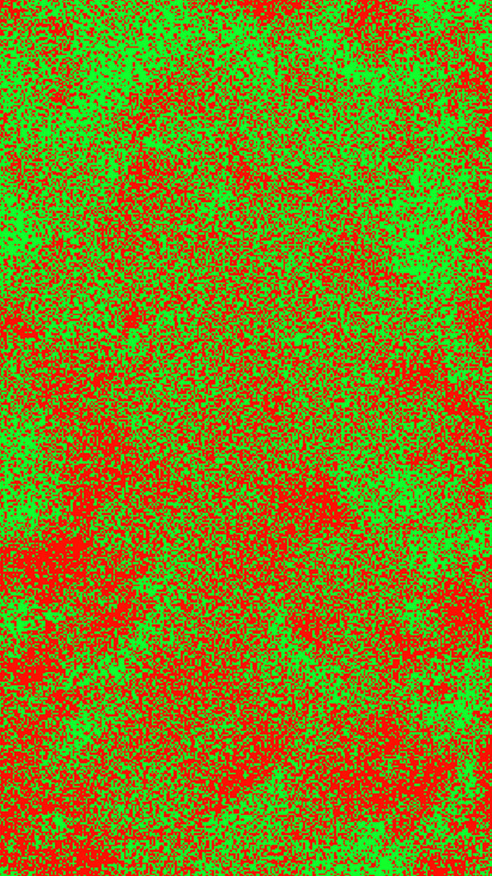
Distribution of high- and low-SF preference. Each imaging pixel has been subdivided into 5 × 5 subpixels, and each subpixel has been colored red (low-SF preference) or green (high-SF preference) at random but so that the appropriate fraction of h(k) response for the pixel was achieved. This is an equivalent representation of the information contained in Fig. 4f.

Each bracketed term of Eq. 4 leads to a preferred orientation map, and these maps are shown in Fig. 4 a and c. The two maps are similar to one another, but there are clear and discernable differences (Fig. 4e). To explore the differences systematically consider Fig. 4 b and d, the amplitude maps associated with the two orientation maps. On each of these maps we have indicated pixels (7% of the total) that come from the tails of the Gaussian distribution shown in Fig. 4f. Red contours surround regions of low-SF preference, and green contours surround regions of high-SF preference. In virtually all cases, the low-k (or high-k) orientation maps contain small regions of robust, pure low-k (or high-k) activity. The same regions contain fractures (i.e., linear loci of discontinuity in preferred orientation) in the complementary high-k (or low-k) maps. To a lesser extent, there are associations of the extreme pixels with pinwheel centers, as expected from the fact that response there tends to zero. It is worth noting that the high- and low-k orientation maps do not share fractures, which might be regarded as evidence of independence. Another discernible difference in the two maps is the presence of small areas for which the preferred orientation of pixels differs by >45° between the high- and low-k orientation maps. These account for ≈12% of the pixels and are not significant because they tend to occur in regions of poor response.

Extensions. In approximating Eq. 2 by the reduced form given by Eq. 3, we have considered those modes that capture the most energy (≈95%) in the signal. It is noteworthy that Eq. 2 has, potentially, more information content. As is clear from Fig. 2, essentially just second harmonics appear in Eq. 3. These second harmonics are enough to determine preferred orientation but not orientation tuning, which requires the above-mentioned fourth harmonics. Similarly, we found two SF frequency functions, α₁(k) and α₃(k), which in turn gave rise to h(k) and l(k). In principle, the number of SF functions, α_n(k), is limited only by the resolution of SF sampling in experiments. Additional SF functions would only modify the SF distribution for a pixel. In general, the distribution of SF preferences for a pixel will be given by a sum over all of the SF functions generated by the data. For Eq. 3 just two dominate but, generally, more can play a role. A unique admixture of all SF functions specifies the SF preference of a single pixel.

These observations can be more fully appreciated in the framework of the concrete model proposed by De Valois and De Valois (17). As shown in the supporting information, application of SVD, Eq. 2, to the model results in a form having coefficients that are exactly factorable. Because the data generated by the model are virtually noise-free, many more terms can be carried in the counterpart of Eq. 3. For example, fourth harmonics yield the inputted tuning width, and higher-order SF eigenfunctions clearly contribute. (See the supporting information for further observations and maps demonstrating convergence to the model itself.)

Comparison with Previous Studies

There have been three key optical-imaging studies that sought to represent SF selectivity in V1 (20, 23, 24). We now compare the results of each of the prior studies with the present results.

In Shoham et al. (20) and related studies (7, 21, 22), orientation images at different SFs were pooled, and maps were obtained by taking their ratios (equivalent to differential imaging). Issa et al. (24) already have shown that such procedures lead to a disproportionate emphasis on high and low SF. As mentioned, pooling over SF generally leads to contamination by the nonspecific response. Because the nonspecific response dominates the specific response, this leads to even more emphasis on high and low SF. In another vein, we point out that the Shoham et al. (20) studies produced putative SF maps with characteristic features on the order of 1 mm. We performed an analysis on our data, in a manner equivalent to that used by Shoham et al. (20), namely without removal of the nonspecific response from our SF maps, and then we followed their procedures for constructing ratios. The result was consistent with that reported by Shoham et al. (20) (see Fig. 6), namely, we obtained blob-like shapes similar in scale to what they interpreted as SF columns.

Substantial use of SVD was made in Everson et al. (23) but without the decomposition shown in Eq. 2. In their study, SFs were pooled, which therefore places the results in doubt. Because their raw data were available to us, we were able to reanalyze them by the methods of the present article. This reanalysis produced results consistent with those reported here (see Figs. 7–10). The two SF functions we obtained have some features in common with the two presented in figure 1j of Everson et al. (23) but are, by and large, significantly different. Despite their concerted effort to remove artifacts, we conclude that the nonspecific response was still present in their results.

Unlike Issa et al. (24), we do not find that orientation pinwheels are loci of either high or low SF [also see Hubener et al. (21)]. We were able to explore this discrepancy because these authors generously furnished us with the data reported in Issa et al. (24). We were given single-condition maps for two of their cat experiments. The data we received already were averaged, and we were not able to apply the GIFA procedure. Although Issa et al. (24) made an effort to remove what we term the nonspecific response, a direct application of SVD analysis to their data demonstrates that they were not entirely successful.

As shown in Fig. 11, vasculature continued to play a dominant role. This finding led us to reprocess their data along the lines indicated in Eq. 1. Although the GIFA procedure could not be performed, we could remove the average map over all eight orientations separately at each SF. This process furnished us with an equivalent to r(k, θ, x) for the Issa et al. (24) data. A decomposition of the form shown in Eq. 2 gave rise to just two significant eigenfunctions, at virtually equal eigenvalues. The coefficients a₁(k, θ) and a₂(k, θ) were both ≈97% factorable. The orientation curves are nicely sinusoidal, and the two SF functions are again almost identical. All of this is in keeping with our results. The peak SF is in agreement with figure 9e of Issa et al. (24) (see Fig. 11 for details).

Discussion

The view that SF preference, in V1, is organized as an admixture of high- and low-frequency distributions resulted from a simple transformation of the naturally occurring functions, {α_n(k)}, and gave us a convenient way by which to regard the results. As indicated previously, the distribution of SF preference in a pixel may be modified by additional SF functions when resolution and signal strength permit these.

As is well known, V1 receives LGN input from X and Y cells, which themselves carry high- and low-SF input from retina with a ratio of ≈3:1 in optimal SF (37, 38), which is similar to the ratio observed for our data (Fig. 3).∥ Tolhurst and Thompson (13) studied the distribution and variety of SF selectivity in the primary visual cortex of cat and found a range of preferred SFs that is comparable to that found in LGN. In Fig. 3, we show SF tuning of two cells (redrawn from their figure 1). In comparing the narrow single-electrode tuning curves with our broader tuning curves in Fig. 3, it is important to bear in mind that for a given retinal eccentricity, the functions h(k) and l(k) likely represent population averages and as such should be broader than single-unit tuning curves (cf. figure 6.1 of ref. 17).

Lack of columnar structure in the SF layout is consistent with the limited experimental results that have been reported. There is anatomical evidence that X and Y streams enter V1 in different, but nearby, layers (40, 41). Optical imaging is unable to resolve such stratification and would show high and low SF as being intermingled. The lack of columnar SF organization in Fig. 5 also is consistent with a variety of electrophysiological accounts that have been reported. For example, Tolhurst and Thompson (14) concluded from their electrophysiological recordings that “organization for optimal SF is neither columnar nor laminar.” De Angelis et al. (16) found pairwise correlations in preferred SF from cortical multiunit recordings, but these occur on scales that are on the order of our imaging pixels (60 μm). Maffei and Fiorentini (42) found significant variation in SF preference in vertical penetrations in V1, which might be indicative of stratification of LGN X and Y input, although Tolhurst and Thompson (14) were not able to replicate this observation.

A Model

We conclude with a speculation, in the form of a model, which fits the results of our analysis and has been hinted at in the prior studies mentioned above.

We start with the anatomical observation that LGN X and Y streams synapse in nearby V1 layers (40, 41) and, perhaps, even in the same layer. This limited evidence indicates twice as many X as Y afferents to V1, which is offset by the observation that there is twice as much Y arborization as X (40, 41). [Reservations about the role of Y input to area 17 have been expressed (43, 44), but the recent article by Yeh et al. (39) appears to have resolved the issue.] These proportions are in agreement with the transformation given by Eq. 4.

The basic premise of our speculation is that the two streams might maintain some limited integrity as subnetworks. The impact of this arrangement would be that orientation preference can be established separately by each subnetwork. There are presently at least two views of how orientation preference is established (45). Under the feedforward orientation model (46, 47), our speculation suggests that X and Y streams each establish oriented on–off Gabor (48, 49) patterns in the primary visual cortex. Under the recurrent orientation model (30, 50, 51), orientation preference is established by disparate orientation opponency. In keeping with our speculation, we point out that this computation might be carried out efficiently by subnetworks because each network operates in only a part of the entire SF range.

Under the proposed model, the h(k) and l(k) distributions might be a consequence of the X and Y subnetworks, each of which establishes its own orientation preference patterns (as typified by Fig. 4 a and c). However, as is well known, SF tuning curves in cortex are band-pass (17), unlike the relatively low-pass SF curves in the LGN. Ringach and colleagues (36, 52) have demonstrated, in macaque, the presence of cortical interactions involving SF preference, and they have argued that this underlies the cortical shaping of SF tuning. Application of these deliberations to our model suggest interactions between the h(k) and l(k) populations of like-orientation preference. Issues of wiring then would argue for the two subnetworks to be similarly aligned, or correlated, in regard to orientation preference, as indeed Fig. 4 a and c are. A consequence of this arrangement would be images that have h(k) and l(k) neurons in close proximity, as depicted in Fig. 5. There would be little reason to expect SF columns in such a framework.

It is important to observe that the evidence for segregated X/Y cortical targets is scant. It may be the case that X and Y LGN afferents do not target different cortical cells. In this event, there would be only one network, and a model of it would need to account for the complementary structure of Fig. 4 b and d.

Conclusions

We contend that the intrinsic optical signal in response to the presentation of a stimulus is contaminated by a component that we have termed the nonspecific response. We have presented a procedure, free of any subjective cosmetic manipulation (e.g., band-pass or Gaussian filtering), for removing this contaminant in the context of a study of orientation and SF preference in the cat primary visual cortex. We stress, however, that this procedure is general and can be applied to the analysis of other types of optical imaging, and possibly functional MRI, experiments. Further analysis of the cleansed response leads to the result that SF preference appears not to be organized in a columnar fashion. Rather, we are led to the speculation that each imaging pixel contains the response from an admixture of high- and low-SF distributions. If there is indeed some linkage in the layout of SF and orientation, it will require more analysis.

We have presented a speculative model, based on previous anatomical and physiological findings, that suggests that our results may be consistent with the view that SF tuning of single cells in the primary visual cortex is shaped by interactions between high- and low-SF populations, which could originate in the X and Y streams incident from the LGN. However, our results do not exclude a single network model, and further experimentation is needed.

References

- 1.Campbell, F. & Robson, J. (1968) J. Physiol. 197, 551-556. [DOI] [PMC free article] [PubMed] [Google Scholar]
- 2.Ginsburg, A. (1971) IEEE Trans. Aerosp. Electron. Syst. 71-C, 283-290. [Google Scholar]
- 3.LeVay, S. & Nelson, S. (1991) in The Neural Basis of Visual Function, ed. Leventhal, A.G. (CRC, Boston), pp. 266-315.
- 4.Thompson, I., Kossut, M. & Blakemore, C. (1983) Nature 301, 712-715. [DOI] [PubMed] [Google Scholar]
- 5.Anderson, P., Olavarria, J. & Van Sluyters, R. (1988) J. Neurosci. 8, 2183-2200. [DOI] [PMC free article] [PubMed] [Google Scholar]
- 6.Blasdel, G. (1992) J. Neurosci. 12, 3115-3138. [DOI] [PMC free article] [PubMed] [Google Scholar]
- 7.Bonhoeffer, T. & Grinvald, A. (1991) Nature 353, 267-294. [DOI] [PubMed] [Google Scholar]
- 8.Sirovich, L., Everson, R., Kaplan, E., Knight, B., O'Brien, E. & Orbach, D. (1996) Physica D 96, 355-366. [Google Scholar]
- 9.Bosking, W., Zhang, Y., Schofield, B. & Fitzpatrick, D. (1997) J. Neurosci. 17, 2112-2127. [DOI] [PMC free article] [PubMed] [Google Scholar]
- 10.Mountcastle, V. (1957) J. Neurophysiol. 20, 408-434. [DOI] [PubMed] [Google Scholar]
- 11.Hubel, D. & Wiesel, T. (1962) J. Physiol. (London) 160, 106-154. [DOI] [PMC free article] [PubMed] [Google Scholar]
- 12.Movshon, J., Thompson, I. & Tolhurst, D. (1978) J. Physiol. (London) 283, 79-99. [DOI] [PMC free article] [PubMed] [Google Scholar]
- 13.Tolhurst, D. & Thompson, I. (1981) Proc. R. Soc. London B 213, 183-199. [DOI] [PubMed] [Google Scholar]
- 14.Tolhurst, D. & Thompson, I. (1982) Exp. Brain Res. 48, 217-227. [DOI] [PubMed] [Google Scholar]
- 15.Tootell, R., Silverman, M. & De Valois, R. (1981) Science 214, 813-815. [DOI] [PubMed] [Google Scholar]
- 16.De Angelis, G., Ghose, G., Ohzawa, I. & Freeman, R. (1999) J. Neurosci. 19, 4046-4064. [DOI] [PMC free article] [PubMed] [Google Scholar]
- 17.De Valois, R. & De Valois, K. (1988) Spatial Vision (Oxford Univ. Press, Oxford).
- 18.Basole, A., White, L. & Fitzpatrick, D. (2003) Nature 423, 986-990. [DOI] [PubMed] [Google Scholar]
- 19.Bonhoeffer, T., Kim, D.-S., Malonek, D., Shoham, D. & Grinvald, A. (1995) J. Neurosci. 7, 1973-1988. [DOI] [PubMed] [Google Scholar]
- 20.Shoham, D., Hubener, M., Schulze, S., Grinvald, A. & Bonhoeffer, T. (1997) Nature 385, 529-533. [DOI] [PubMed] [Google Scholar]
- 21.Hubener, M., Shoham, D., Grinvald, A. & Bonhoeffer, T. (1997) J. Neurosci. 17, 9270-9284. [DOI] [PMC free article] [PubMed] [Google Scholar]
- 22.Bonhoeffer, T. & Grinvald, A. (1993) J. Neurosci. 13, 4157-4180. [DOI] [PMC free article] [PubMed] [Google Scholar]
- 23.Everson, R., Prashanth, A., Gabbay, M., Knight, B., Sirovich, L. & Kaplan, E. (1998) Proc. Natl. Acad. Sci. USA 95, 8334-8338. [DOI] [PMC free article] [PubMed] [Google Scholar]
- 24.Issa, N., Trepel, C. & Stryker, M. (2000) J. Neurosci. 20, 8504-8514. [DOI] [PMC free article] [PubMed] [Google Scholar]
- 25.Bressloff, P., Cowan, J., Golubitsky, M., Thomas, P. & Wiener, M. (2001) Philos. Trans. R. Soc. London B 356, 299-330. [DOI] [PMC free article] [PubMed] [Google Scholar]
- 26.Sirovich, L. & Kaplan, E. (2002) in In Vivo Optical Imaging of Brain Function, ed. Frostig, R. D. (CRC, Boca Raton, FL), pp. 43-76.
- 27.Frostig, D., Lieke, E., Ts'o, D. & Grinvald, A. (1990) Proc. Natl. Acad. Sci. USA 87, 6082-6086. [DOI] [PMC free article] [PubMed] [Google Scholar]
- 28.Malonek, D. & Grinvald, A. (1996) Science 272, 551-554. [DOI] [PubMed] [Google Scholar]
- 29.Yokoo, T. (2003) Ph.D. thesis (Mount Sinai School of Medicine, New York).
- 30.Troyer, T., Krukowski, A., Priebe, N. & Miller, K. (1998) J. Neurosci. 18, 5908-5927. [DOI] [PMC free article] [PubMed] [Google Scholar]
- 31.Geisler, W. & Albrecht, D. (1997) Visual Neurosci. 14, 897-919. [DOI] [PubMed] [Google Scholar]
- 32.Ferster, D. & Miller, K. (2000) Annu. Rev. Neurosci. 23, 441-471. [DOI] [PubMed] [Google Scholar]
- 33.Hammond, P. & Pomfrett, C. (1990) Vision Res. 30, 359-369. [DOI] [PubMed] [Google Scholar]
- 34.Webster, M. & De Valois, R. (1985) J. Opt. Soc. Am. A 2, 1124-1132. [DOI] [PubMed] [Google Scholar]
- 35.Mazer, J., Vinje, W., McDermott, J., Schiller, P. & Gallant, J. (2002) Proc. Natl. Acad. Sci. USA 99, 1645-1650. [DOI] [PMC free article] [PubMed] [Google Scholar]
- 36.Ringach, D., Bredfeldt, C., Shapley, R. & Hawken, M. (2002) J. Neurophysiol. 87, 1018-1027. [DOI] [PubMed] [Google Scholar]
- 37.Derrington, A. & Fuchs, A. (1979) J. Physiol. (London) 293, 347-364. [DOI] [PMC free article] [PubMed] [Google Scholar]
- 38.So, Y. & Shapley, R. (1979) Exp. Brain Res. 36, 533-550. [DOI] [PubMed] [Google Scholar]
- 39.Yeh, C.-I., Stoelzel, C. & Alonso, J.-M. (2003) J. Neurophysiol. 90, 1852-1864. [DOI] [PubMed] [Google Scholar]
- 40.Humphrey, A., Sur, M., Uhlrich, D. & Sherman, S. (1985) J. Comp. Neurol. 233, 159-189. [DOI] [PubMed] [Google Scholar]
- 41.Freund, T., Martin, K. & Whitteridge, D. (1985) J. Comp. Neurol. 242, 263-274. [DOI] [PubMed] [Google Scholar]
- 42.Maffei, L. & Fiorentini, A. (1977) Vision Res. 17, 257-264. [DOI] [PubMed] [Google Scholar]
- 43.Ferster, D. (1990) Visual Neurosci. 4, 115-133. [DOI] [PubMed] [Google Scholar]
- 44.Ferster, D. (1990) Visual Neurosci. 4, 135-145. [DOI] [PubMed] [Google Scholar]
- 45.Sompolinsky, H. & Shapley, R. (1997) Curr. Opin. Neurobiol. 7, 514-522. [DOI] [PubMed] [Google Scholar]
- 46.Ferster, D., Chuing, S. & Wheat, H. (1996) Nature 380, 249-252. [DOI] [PubMed] [Google Scholar]
- 47.Reid, R. & Alonso, J.-M. (1996) Curr. Opin. Neurobiol. 6, 475-480. [DOI] [PubMed] [Google Scholar]
- 48.DeAngelis, G., Ohzawa, I. & Freeman, R. (1993) J. Neurophysiol. 69, 1091-1117. [DOI] [PubMed] [Google Scholar]
- 49.DeAngelis, G., Ohzawa, I. & Freeman, R. (1993) J. Neurophysiol. 69, 1118-1135. [DOI] [PubMed] [Google Scholar]
- 50.Somers, D. Nelson, S. & Sur, M. (1995) J. Neurosci. 15, 5448-5465. [DOI] [PMC free article] [PubMed] [Google Scholar]
- 51.Omurtag, A., Kaplan, E., Knight, B. & Sirovich, L. (2000) Network 11, 247-260. [PubMed] [Google Scholar]
- 52.Bredfeldt, E. & Ringach, D. (2002) J. Neurosci. 22, 1976-1984. [DOI] [PMC free article] [PubMed] [Google Scholar]
Associated Data
This section collects any data citations, data availability statements, or supplementary materials included in this article.