Meta‐analysis of few small studies in orphan diseases

Abstract

Meta‐analyses in orphan diseases and small populations generally face particular problems, including small numbers of studies, small study sizes and heterogeneity of results. However, the heterogeneity is difficult to estimate if only very few studies are included. Motivated by a systematic review in immunosuppression following liver transplantation in children, we investigate the properties of a range of commonly used frequentist and Bayesian procedures in simulation studies. Furthermore, the consequences for interval estimation of the common treatment effect in random‐effects meta‐analysis are assessed. The Bayesian credibility intervals using weakly informative priors for the between‐trial heterogeneity exhibited coverage probabilities in excess of the nominal level for a range of scenarios considered. However, they tended to be shorter than those obtained by the Knapp–Hartung method, which were also conservative. In contrast, methods based on normal quantiles exhibited coverages well below the nominal levels in many scenarios. With very few studies, the performance of the Bayesian credibility intervals is of course sensitive to the specification of the prior for the between‐trial heterogeneity. In conclusion, the use of weakly informative priors as exemplified by half‐normal priors (with a scale of 0.5 or 1.0) for log odds ratios is recommended for applications in rare diseases. © 2016 The Authors. Research Synthesis Methods published by John Wiley & Sons Ltd.

1. Introduction

In the European Union, a disease affecting 5 in 10 000 people is considered rare, whereas in the USA, a condition affecting fewer than 200 000 people is defined as rare. As these examples show, no universal definition of rare diseases (also referred to as orphan diseases) exists (Aronson, 2006). It is estimated that 6000 to 8000 rare diseases are known today, with numbers increasing as more diseases are discovered. Many of these have a genetic component, are chronic as well as life‐threatening and affect children (refer to e.g. rarediseases.org or www.orpha.net). Examples of rare diseases include childhood cancers, amyotrophic lateral sclerosis and Creutzfeldt–Jacob disease. More generally, small populations can occur by rare conditions or by stratification of more common diseases by, for example, genetic markers.

Because rare diseases and small populations pose particular problems to design, conduct and analysis of clinical research as a result of the small sizes, various efforts have been undertaken in tailoring methods specific for the application in these populations (Gagne et al., 2014). Recent publications such as Hampson et al. (2014) and Speiser et al. (2015) demonstrate that this is an ongoing effort, which is also reflected in a recent funding initiative of the European Commission supporting three research networks in developing clinical research methodology suitable for rare diseases and small populations, namely “Integrated Design and Analysis of Small Population Group Trials”, “Advances in Small Trials Design for Regulatory Innovation and Excellence” and “Innovative Methodology for Small Population Research”. Also, regulatory authorities acknowledge the need for innovative approaches to clinical trials in rare and very rare diseases (European Medicines Agency (EMEA), 2006). To our knowledge, however, neither have the standard methods of meta‐analysis been assessed for their suitability to be applied in small populations and rare diseases nor have any specific methods for meta‐analysis been developed for these populations. This is surprising, because it is generally accepted that meta‐analytic methods are a powerful tool to guide objective decision‐making by allowing for the formal, statistical combination of information to merge data from individual experiments to a joint result.

There are some specific challenges for meta‐analyses in small populations and rare diseases. As will be seen in the motivating example of Section 2, the number of studies included in meta‐analyses is typically small, and the studies themselves are rather small, with many of them being inconclusive. In this situation, a formal synthesis of the available evidence is highly desirable. However, the study designs often vary, for instance, with regard to the type of control groups (historical vs. concurrent controls) and treatment allocation (non‐randomized vs. randomized; allocation ratio), making between‐trial heterogeneity with regard to the treatment effects very likely. In fact, smaller studies have empirically been found to exhibit more heterogeneity than large ones (IntHout et al., 2015). The situation gets even more difficult for rare events (Sweeting et al., 2004; Bradburn et al., 2007; Kuß, 2015), but this is not our scope here.

Many meta‐analyses may be approached using approximately normal effect estimates and a normal random‐effects model, the normal–normal hierarchical model (NNHM) (Hedges and Olkin, 1985). The between‐study heterogeneity plays a central role in this context. Estimation of the heterogeneity variance component based on only a few studies, however, is particularly challenging, as the resulting uncertainty is often substantial and consistent with small to large heterogeneity. Proper accounting for this uncertainty is crucial when estimating effect sizes. Especially when the analysis is based on few studies, which is a common problem not only for orphan diseases, the utilization of a priori information on heterogeneity may be helpful (Sutton and Abrams, 2001).

Our aim is to assess the properties of Bayesian and popular frequentist methods in a simulation study covering typical scenarios for rare disease as well as in a case study. We have developed a method to substantially ease the computational burden of a Bayesian random‐effects meta‐analysis, which avoids Markov chain Monte Carlo computations and facilitates large‐scale simulations. The method has been implemented in the R package bayesmeta publicly available for download from CRAN (Röver, 2015).

The paper is organized as follows. In Section 2, we introduce a case study in paediatric transplantation, motivating our investigations. In Section 3, the statistical model as well as the methods for meta‐analysis are introduced and are compared in a simulation study in Section 4. The findings are illustrated by revisiting the systematic review in paediatric transplantation in Section 5. We close with a brief discussion.

2. A case study in paediatric transplantation

Several rare paediatric liver diseases can nowadays be successfully treated by liver transplantation with good long‐term outcomes (Spada et al., 2009; Kosolo, 2013). One key component of a successful treatment is effective and safe immunosuppression after transplantation. A number of immunosuppressant drugs with different mechanisms of action and associated adverse event profiles are available and are given either as monotherapy or in combination (for an overview, refer to e.g. Table 1 in Kosolo, 2013). Relatively new are the Interleukin‐2 receptor antibodies (IL‐2RA) Basiliximab and Daclizumab. Recently, Crins et al. (2014) conducted a systematic review of controlled but not necessarily randomized studies of IL‐2RA in paediatric liver transplantation. Primary outcomes were acute rejections (ARs), steroid‐resistant rejections (SRRs), graft‐loss and death. For illustrative purposes, we focus here on ARs and SRRs. A total of six studies (Heffron et al., 2003; Gibelli et al., 2004; Schuller et al., 2005; Ganschow et al., 2005; Spada et al., 2006; Gras et al., 2008) were included in a meta‐analysis assessing the risk of acute rejections on treatments with IL‐2RA in comparison with control, whereas only three of these six studies reported data on steroid‐resistant rejections.

Table 1.

Between‐trial heterogeneity for log‐odds ratios: τ values representing small to very large heterogeneity, with 95% intervals for across‐trial odds ratios (exp (θ_j)).

Heterogeneity		95% interval
Small:	τ = 0.125	0.783–1.28
Moderate:	τ = 0.25	0.613–1.63
Substantial:	τ = 0.5	0.325–2.66
Large:	τ = 1	0.141–7.10
Very large:	τ = 2	0.020–50.4

Crins et al. used the DerSimonian–Laird (DerSimonian and Laird, 1986) method and the restricted maximum‐likelihood (REML) approach to estimate the between‐study variance. Although they reported treatment effects in terms of relative risks, we use here the odds ratio, as it is the more commonly used measure. Figure 1 gives the numbers of patients and events by treatment group and depicts the odds ratios comparing IL‐2RA treatment with control in forest plots. The 95% confidence intervals (CIs) of the odds ratios were computed using normal approximation on the log‐scale (zero cell entries here were treated by adding $\frac{1}{2}$ to each cell of the corresponding contingency table).

Figure 1.

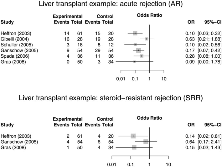
Forest plots of odds ratios for acute rejections and steroid‐resistant rejections based on data from the systematic review by Crins et al. (2014).

The specific problems with meta‐analyses in rare diseases outlined in Section 1 are prominent here. First, the number of controlled studies is with 6 and 3 rather small, although the search was not restricted to randomized studies only. Second, the total sample sizes varied from only 30 to 108. Third, there are some marked differences in the designs employed. For instance, only the studies by Heffron (2003) and Spada (2006) were randomized, and some of the non‐randomized studies used concurrent controls, whereas others relied on historical control data. Finally, the allocation ratios ranged between 1:1 and 3:1. These variations in design lead to some heterogeneity in the results as is apparent from the forest plots. In the next section, we will summarize a number of methods to quantify this heterogeneity.

3. Methods

The vast majority of meta‐analyses use common effect (fixed‐effect) or random‐effects models. For the latter, the NNHM is the most popular. It has two parts: a sampling and a parameter model. The sampling model assumes approximately normally distributed estimates Y ₁, …, Y _k for the trial‐specific parameters θ ₁, …, θ _k

$$Y_{\mathrm{j}}|{\theta }_{\mathrm{j}}\sim N\left({\theta }_{\mathrm{j}},s_{\mathrm{j}}^2\right),j=1,\dots ,k\text{.}$$ (1)

Any estimation uncertainty in the standard errors s _j is neglected here. The parameter model softens the strong (common effect) assumption of parameter equality to parameter similarity. The simplest similarity model assumes the parameters as random (or exchangeable) effects

$${\theta }_{\mathrm{j}}|\mu ,\tau \sim N\left(\mu ,{\tau }^2\right),j=1,\dots ,k\text{.}$$ (2)

Equivalently, this model introduces a variance component for between‐trial variability, θ _j = μ + ε_j, with ε_j ∼ N(0, τ ²). The between‐trial standard deviation τ determines the degree of similarity across parameters; the special case τ = 0 corresponds to the common effect model.

The scope of the NNHM is broad. The focus can be on the trial‐specific parameters θ _j, the predicted parameter θ _k + 1 in an new trial or the mean parameter μ. Here, we will be concerned with the latter. For this case, inference can be simplified by considering only the marginal model

$$Y_{\mathrm{j}}|\mathrm{\mu },\tau \sim N\left(\mathrm{\mu },s_{\mathrm{j}}^2+{\tau }^2\right),j=1,\dots ,k\text{.}$$ (3)

The two ways to infer the parameter of interest μ and the nuisance parameter τ are classical and Bayesian. If τ were known, they would lead to the same conclusions for μ. Classically,

$$\widehat{\mu }={\displaystyle \sum _{j=1}^k}{w}_{\mathrm{j}}{Y}_{\mathrm{j}}/{\displaystyle \sum _{j=1}^k}{w}_{\mathrm{j}}\sim N\left(\mu ,1/w_{+}\right)$$ (4)

where w _j are the inverse‐variance (precision) weights

$$w_{\mathrm{j}}=1/\left(s_{\mathrm{j}}^2+{\tau }^2\right),j=1,\dots k\text{,}$$ (5)

and the total precision of the estimate is the sum of the marginal precisions, $w_{+}={\displaystyle {\sum }_{j=1}^k{w}_j}$. For known τ and a non‐informative (improper) prior on μ, the Bayesian result is

$$\mathrm{\mu }|Y_1,\dots ,Y_{\mathrm{k}}\sim N\left({\displaystyle \sum _{j=1}^k}{w}_{\mathrm{j}}{Y}_{\mathrm{j}}/{\displaystyle \sum _{j=1}^k}{w}_j,1/w_{+}\right)\text{.}$$ (6)

While this “equivalence” of classical and Bayesian results for μ is comforting, it breaks down if τ is not known. For this case, classical methods to infer μ involve two steps:

1. An estimate $\widehat{\tau }$ is derived, which is then used to obtain the weights (5) and the corresponding estimate for μ in (4).

2. A confidence interval (CI) is derived. In this step, the uncertainty for the estimate $\widehat{\tau }$ is sometimes ignored, that is, the normal approximation in (4) with the plug‐in estimate $\widehat{\tau }$ is used, or the uncertainty of $\widehat{\tau }$ is taken into account, for example, by the t _k − 1 approximation (Follmann and Proschan, 1999), the profile likelihood method (Hardy and Thompson, 1996) or the method by Hartung and Knapp (Hartung and Knapp, 2001a,2001b; Knapp and Hartung, 2003).

For step (i), many methods have been proposed (e.g. DerSimonian and Kacker, 2007; Chung et al., 2013). In the following sections, we will use four estimates:

• DL: The frequently used DerSimonian–Laird estimate (DerSimonian and Laird, 1986) is a moment‐based estimate for τ. The DL estimate does not require distributional assumptions and is available in closed form. However, it tends to underestimate τ. It often leads to zero estimates for τ (particularly for small numbers of trials), and thus results in a common effect meta‐analysis with potentially too optimistic CIs for μ.

• REML: The restricted (or residual) maximum likelihood estimate has been proposed as an improvement over the standard ML estimate (Viechtbauer, 2005). The REML estimate requires iterative computations. It has the advantage of being less downward biased compared with the DL and ML estimates.

• MP: The Mandel–Paule (Paule and Mandel, 1982) estimate provides an approximation to the REML estimate (Rukhin et al., 2000; DerSimonian and Kacker, 2007); like the DL estimate, it does not require distributional assumptions, and it has been recommended for use in meta‐analysis (Veroniki et al., 2015).

• BM: The Bayes modal estimate (Chung et al., 2013) is an example of a hybrid approach. In the first step, it derives a non‐zero Bayesian estimate for τ using a gamma prior with shape parameter α > 1, and then proceeds in a classical way to infer μ in step (2). Effectively, this is a penalized likelihood approach.

For step (ii), we will use two methods to derive CIs for μ for each of the four τ estimates.

• The simple normal approximation (4), which ignores the uncertainty for $\widehat{\tau }$. The 1 − α CI is constructed as $\widehat{\mathrm{\mu }}\pm z_{1-\mathrm{\alpha }/2}{\sigma }_{\mathrm{\mu }}$, where z _γ is the γ‐quantile of the standard normal distribution, and σ _μ is the standard error of $\widehat{\mathrm{\mu }}$ given by ${\sigma }_{\mathrm{\mu }}=\sqrt{\frac{1}{w_{+}}}$.

• The method by Hartung and Knapp (Hartung and Knapp, 2001a,2001b; Knapp and Hartung, 2003). Their method assumes that an estimate $\widehat{\mathrm{\mu }}$ has been obtained (e.g. based on the DL estimate for τ, which also implies weights w _j in (5)). Based on these quantities, the variance estimate for $\widehat{\mathrm{\mu }}$ is obtained as $q{\sigma }_{\mathrm{\mu }}^2$ with

  $$q=\frac{1}{k-1}{\displaystyle \sum _j}{w}_{\mathrm{j}}{\left(y_{\mathrm{j}}-\widehat{\mathrm{\mu }}\right)}^2\text{.}$$ (7)

  The variance estimator $q{\sigma }_{\mathrm{\mu }}^2$ can be interpreted as a weighted extension of the usual empirical variance of the study‐specific estimator. However, there are additional results which make $q{\sigma }_{\mathrm{\mu }}^2$ attractive (Hartung and Knapp, 2001a,2001b; Knapp and Hartung, 2003): $q{\sigma }_{\mathrm{\mu }}^2$ is an unbiased estimate of $\mathrm{V}\mathrm{a}\mathrm{r}\left(\widehat{\mathrm{\mu }}\right)$, and $w_{+}\left(k-1\right)q{\sigma }_{\mathrm{\mu }}^2$ follows a ${\chi }_{\mathrm{k}-1}^2$ distribution. This, in turn, leads to the construction of an 1 − α CI for μ as $\widehat{\mathrm{\mu }}\pm t_{\mathrm{k}-1;1-\mathrm{\alpha }/2}\sqrt{q}{\sigma }_{\mathrm{\mu }}$. Here, we use the modified version, replacing q by q ^⋆ with q ^⋆ = max {1, q} (Röver et al., 2015). Furthermore, this interval provides coverage for μ close to the nominal level (Sidik and Jonkman, 2003), at least when the number of studies is sufficiently large.

In the Bayesian approach, uncertainty about τ is automatically accounted for when estimating μ. However, the choice of prior matters, particularly if the number of studies is small. This case has been discussed in Turner et al. (2015), Section 2 of Dias et al. (2012) and Section 6.2 of Dias et al. (2014). While we suggest to use informative priors for τ if solid information about between‐trial heterogeneity is available, in what follows, we will only consider the case where prior information is weak. For this case, we recommend to use priors that put most of their probability mass to values that represent small to large between‐trial heterogeneity and leave the remaining probability (e.g. 5%) to values that reflect very large heterogeneity. These weakly informative priors can be represented by half‐normal, half‐Cauchy or half‐t distributions (Spiegelhalter et al., 2004; Gelman, 2006; Polson and Scott, 2012).

What constitutes small to large heterogeneity depends on the parameter scale. The situation we consider here is the two‐group (test vs. control) binomial case with parameters π _Tj and π _Cj for study j. The numbers of patients in the test and control group are denoted by n _Tj and n _Cj respectively, while the numbers of events are denoted by r _Tj and r _Cj. Here the log‐odds ratio θ _j is used for comparison. The corresponding approximate NNHM assumes exchangeable log‐odds ratios across trials

$${\theta }_{\mathrm{j}}=\log \left(\frac{{\pi }_{\mathrm{T}\mathrm{j}}\left(1-{\pi }_{\mathrm{C}\mathrm{j}}\right)}{{\pi }_{\mathrm{C}\mathrm{j}}\left(1-{\pi }_{\mathrm{T}\mathrm{j}}\right)}\right)\sim N\left(\mathrm{\mu },{\tau }^2\right)$$ (8)

and approximately normal log‐odds ratio estimates Y _j with standard errors s _j

$$Y_{\mathrm{j}}=\log \left(\frac{r_{\mathrm{T}\mathrm{j}}\left(n_{\mathrm{C}\mathrm{j}}-r_{\mathrm{C}\mathrm{j}}\right)}{r_{\mathrm{C}\mathrm{j}}\left(n_{\mathrm{T}\mathrm{j}}-r_{\mathrm{T}\mathrm{j}}\right)}\right),s_{\mathrm{j}}^2=1/r_{\mathrm{T}\mathrm{j}}+1/\left(n_{\mathrm{T}\mathrm{j}}-r_{\mathrm{T}\mathrm{j}}\right)+1/r_{\mathrm{C}\mathrm{j}}+1/\left(n_{\mathrm{C}\mathrm{j}}-r_{\mathrm{C}\mathrm{j}}\right)\text{.}$$ (9)

We will use half‐normal priors HN(φ) that cover the range of typical τ values representing small to very large heterogeneity: 0.125 (small), 0.25 (moderate), 0.5 (substantial), 1 (large) and 2 (very large); refer to Section 5.7 in Spiegelhalter et al. (2004). A half‐normal distribution HN(φ) with scale φ results from taking absolute values of observations sampled from a normal distribution with an expectation of 0 and a variance of φ ². To illustrate between‐trial heterogeneity for these τ values, Table 1 shows 95% intervals for across‐trial odds ratios (conditional on μ = 0). In Table 2, the three “weakly informative” priors are shown, which we will use in the following sections. These are two half‐normal priors with scales of 0.5 and 1 and a uniform (0, 4) prior. The latter, which puts 50% prior probability on very large between‐trial heterogeneity (in most cases, a rather unrealistic assumption), will be used to assess prior sensitivity.

Table 2.

Between‐trial heterogeneity for log‐odds ratios: three priors covering small to large heterogeneity.

Prior distribution	Median	95% interval
Half normal (scale = 0.5)	0.337	(0.016, 1.12)
Half normal (scale = 1.0)	0.674	(0.031, 2.24)
Uniform (0, 4)	2.0	(0.1, 3.9)

4. Simulation study

In order to compare the performance of the different approaches to construct credibility or confidence intervals for the treatment effect μ introduced in Section 3, we conducted a simulation study. The simulation scenarios are similar to those considered in Chung et al. (2013) and Brockwell and Gordon (2001) but extend to smaller numbers of studies included in the meta‐analyses and to more pronounced between‐trial heterogeneity to reflect the particular circumstances frequently encountered in small populations and rare diseases. We generated data according to the model described in Section 3, where we varied the number of studies involved (k ∈ {3, 5, 10}), the true heterogeneity present (τ ² ∈ {0, 0.01, 0.02, 0.05, 0.1, 0.2, 0.5, 1.0, 2.0}), and where the individual studies' associated standard errors are generated based on draws from a χ ² distribution as described in Brockwell and Gordon (2001). We then investigated the estimation accuracy for heterogeneity τ and effect μ by logging the resulting estimates (marginal posterior median in case of the Bayesian methods) and the coverage of true values for confidence and credibility intervals. The simulations were carried out with 10 000 replications per scenario.

Because some readers might be more familiar with the I ² measure to capture the extent of heterogeneity than τ ², we report here median values of the simulated I ² depending on τ ² for illustrative purposes. For instance, τ ² = 0.02, 0.10, 0.5, 2 resulted in median I ² of 0.11, 0.37, 0.75 and 0.92.

Figure 2 shows the bias of several estimators of τ, given various numbers of studies k included in the meta‐analyses and a range of true values of τ. The extent of bias strongly depends on the number of studies k for all estimators considered with small bias for large k and substantial bias in situations typically encountered in small population research. Here, the direction and size of bias largely depend on the value of τ itself and the estimator. For small τ, the bias can naturally be only positive. For medium to large between‐trial heterogeneity, the likelihood estimators and the DL estimator tend to underestimate τ, whereas the Bayesian methods tend to overestimate the between‐trial heterogeneity. For very large τ, the picture changes again, with some of the Bayesian methods leading to estimates which are in expectation well below the true value depending on the choice of prior. For large and very large τ, the likelihood‐based estimators and the DL display substantial negative bias.

Figure 2.

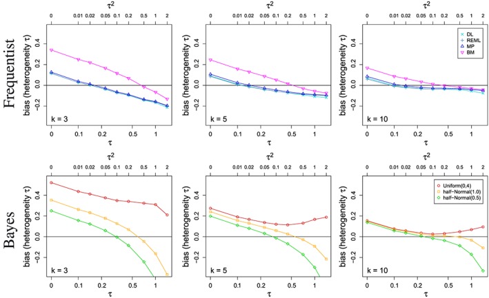
Bias in estimating the between‐study heterogeneity τ for various estimators and for several numbers k of studies included in the meta‐analyses.

For those estimators that are not strictly positive by construction (i.e. DL, REML and MP), Figure 3 shows the proportion of estimates of the between‐study heterogeneity τ equal to zero, depending on the number k of studies included in the meta‐analyses. In particular, for small k, the proportion of estimates being equal to 0 is substantial for small to moderate τ. This effect diminishes with increasing k. As for the bias, the differences between the three estimators are rather small.

Figure 3.

Proportion of estimates of the between‐study heterogeneity τ equal to zero for those estimators that are not strictly positive by construction depending on the number k of studies included in the meta‐analyses.

Given the differences between the seven estimators of τ, one might expect that this would result in differences in estimating μ. Interestingly, we did not observe any marked differences in the root mean squared error for the corresponding estimators of the treatment effect μ, with all differences being below 9% and discrepancies vanishing with increasing τ and larger k (data not shown).

Figure 4 shows the coverage of several credibility and confidence intervals for the treatment effect μ depending on the between‐trial heterogeneity τ ² and the number of included studies k. When considering the bias in estimating τ above, no estimator outperformed the others over the range of the considered scenarios. Comparing the various approaches with regard to the coverage probabilities of the credibility and confidence intervals for μ, however, the picture becomes much clearer. The frequentist methods based on normal approximation achieve coverage probabilities at or above the nominal level only for relatively small τ (i.e. τ ≤ 0.1), for which the Bayesian methods as well as the Knapp–Hartung method are conservative. For most other values of τ, the Bayes and Knapp–Hartung methods outperform the normal approximation approaches in that they provide higher coverage probabilities. However, also for Bayesian and Knapp–Hartung methods, the actual coverage can deviate from the nominal confidence level substantially. With appropriate choice of the prior distribution, the coverage probabilities of the Bayesian credibility intervals are often closer to the nominal level than the Knapp–Hartung method. The differences between the various methods are not only a result of differences in estimating τ but also reflect differences in the construction of the intervals. By construction, the Bayesian credibility intervals are guaranteed to produce coverage probabilities of the nominal level when averaged over the prior distribution. Here, we consider coverage probabilities at fixed τ, and therefore expect the coverage probabilities to vary with τ. The frequentist methods considered achieve the coverage probability asymptotically, but their characteristics for finite samples are not obvious. This can be seen in Figure 4, where the coverage probabilities are closer to the nominal level for larger k.

Figure 4.

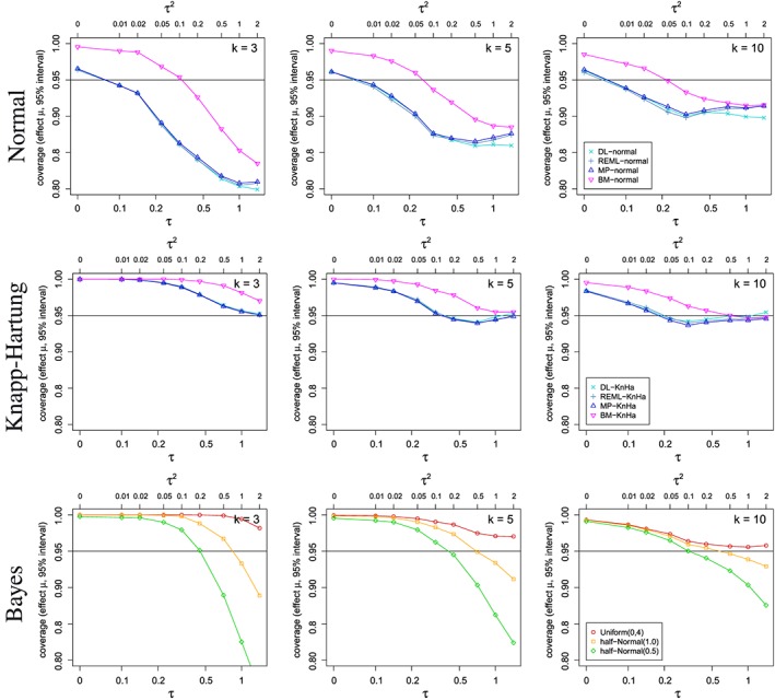
Coverage probability for credibility/confidence intervals for the overall treatment effect μ depending on the between‐study heterogeneity τ and several numbers k of studies included in the meta‐analyses using various estimators.

Figure 5 shows the simulated mean lengths of several credibility and confidence intervals for the treatment effect μ depending on the between‐trial heterogeneity τ ² and the number of included studies k. By construction, the CIs based on normal approximation are shorter than the Knapp–Hartung intervals. The Bayesian intervals tend to be shorter than the Knapp–Hartung intervals, also in situations with similar or even larger coverage probability.

Figure 5.

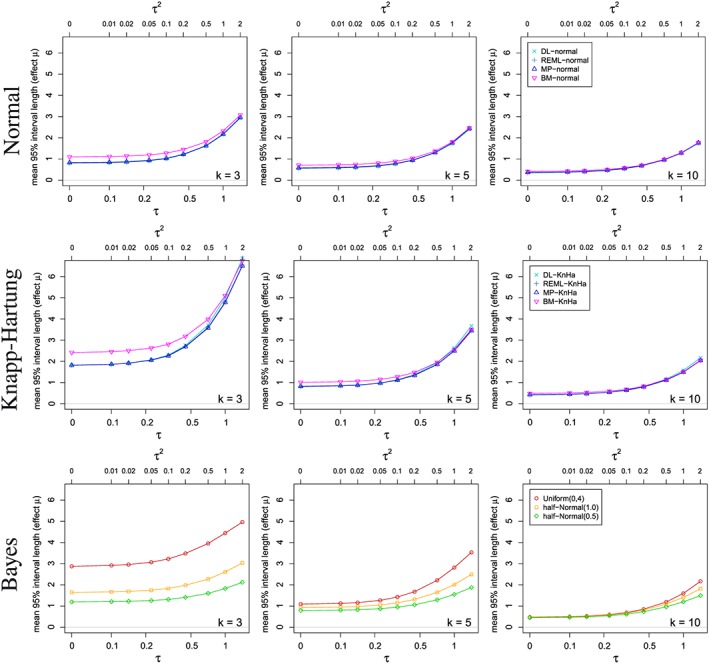
Mean lengths of the credibility/confidence intervals for the overall treatment effect μ depending on the between‐study heterogeneity τ and several numbers k of studies included in the meta‐analyses using various estimators.

In conclusion, the method based on normal quantiles cannot be recommended for use with small numbers of studies because the observed coverage was often well below the nominal level. The Knapp–Hartung approach leads to coverage at or above the nominal level, but in cases with very few studies results in extremely long CIs. Bayesian credibility intervals with appropriate choice of prior performed well and can be recommended for application in rare diseases. However, with very small number of studies included, the results are sensitive to the prior specification.

5. The motivating case study revisited

In this section, we are returning to the case study by Crins et al. (2014) introduced in Section 2. Crins et al. investigated immunosuppressive therapies in paediatric liver transplantation with regard to acute and steroid‐resistant rejections. In the first part of this section, we will apply the methods introduced in Section 3 to these data and discuss the results. In the second part, we will investigate the long‐run behaviour of the different meta‐analysis procedures based on scenarios motivated by the liver transplant example simulating binomial data rather than normal test statistics and their standard errors. Although simulating from binomial distributions, we will keep to the standard NNHM for analysis. Alternatively, one could model the counts directly using binomial distributions (Spiegelhalter et al., 2004; Böhning et al., 2008; Kuß, 2015).

Figure 6 shows the results of applying the various methods introduced in Section 3 to the paediatric liver transplant data presented in Section 2. In the figure, the treatment effect estimates are shown on the log‐odds ratio scale with 95% CI for the individual studies as well as for the meta‐analyses. The estimates $\widehat{\tau }$ of the between‐trial heterogeneity are also included in the figure. For the Bayes methods, the posterior medians are given. Whereas in the case of acute rejections, the results are fairly similar across the various methods with statistically significant combined treatment effects as reported in Crins et al. (2014), there are some marked differences between the methods in the case of steroid‐resistant rejections. On the whole, the methods based on normal approximation lead to the shortest CIs, which are indicating statistically significant effects with the exception of the BM method. The Knapp–Hartung approach leads to intervals including 0 independent of the heterogeneity estimation method and are among the longest intervals obtained. With only three studies included in the SRR meta‐analyses, the differences between the Knapp–Hartung and the normal approaches are more pronounced than in the AR example. In this example, the Bayes methods provide a middle ground with credibility intervals which are on the whole shorter than those obtained by the Knapp–Hartung method and upper credibility limits close to 0, with the only exception being the estimate based on the conservative uniform prior. However, because of the very small number of studies, the Bayes estimators are more sensitive to the specification of prior than in the AR example with six trials.

Figure 6.

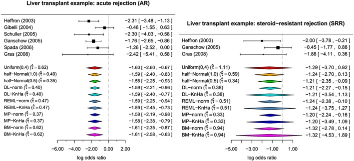
Paediatric transplant example: Treatment effect estimates on the log‐odds ratio scale with 95% confidence intervals for the individual studies and meta‐analyses as well as estimates $\widehat{\tau }$ of the between‐trial heterogeneity. For the Bayes methods, the posterior medians are given.

In the AR example, the estimates of the between‐trial heterogeneity τ centre around 0.5 and vary from 0.37 with the MP estimator to 0.62 for the BM estimator and the Bayes estimator with uniform prior on the interval from 0 to 4. In the SRR data, the observed heterogeneity is somewhat higher in comparison with estimates ranging from 0.33 for the MP estimator to 1.11 for the Bayes estimator with uniform prior. All these estimates come with a considerable degree of uncertainty reflected in the length of the confidence/credibility intervals. For the acute rejections, the 95% credibility intervals of τ are 0 to 1.848 with uniform prior, to 1.260 with half‐normal prior with scale 1, and to 0.862 for half‐normal prior with scale 0.5, whereas the 95% CI using the Q‐profile method extends from 0 to 1.726. For the steroid‐resistant rejections, the 95% credibility intervals range from 0 to 3.368, 1.652 and 0.941 for the uniform and the two half‐normal priors with scales 1 and 0.5 respectively. The 95% Q‐profile interval even extends from 0 to 5.365. As can be seen from this example, the credibility intervals depend very much on the choice of prior, particularly with very small numbers of studies. The frequentist Q‐profile method gives CIs as wide or as wider than the credibility intervals based on the conservative uniform prior.

We exemplarily investigated the long‐run behaviour of the different meta‐analysis procedures based on scenarios motivated by the liver transplant example. For this purpose, we simulated data similar to the meta‐analyses of acute rejections and steroid‐resistant rejections. The former included six studies; the latter included only three. In each simulation iteration, first true group‐specific odds were generated as normally distributed on the log‐odds scale; for AR with means μ_control = 0.0 and μ_treatment = − 1.5 and for SR with μ_control = − 2.0 and μ_treatment = − 3.0. Variances were equal to 1, and the log‐odds were positively correlated with correlation coefficients 0.875 and 0.719 for AR and SRR respectively. The resulting between‐trial heterogeneity in terms of log‐odds ratios is τ = 0.5 for AR and τ = 0.75 for SRR, which are substantial and substantial to large levels of heterogeneity according to Table 1. Resulting log‐odds were then used to generate study results (contingency tables) based on a binomial distribution and patient numbers as given in the examples. The corresponding effect size estimates and standard errors were computed using the escalc() function from the metafor package (Viechtbauer, 2010), which were then analysed using the different methods. The results of these simulations are summarized in Table 3, where the coverage probabilities and mean lengths of the 95% CIs for the treatment effect μ are given. As with the simulation study presented in Section 4, 10 000 trials were simulated for each scenario.

Table 3.

Comparison of different methods using simulations of binary data imitating the example settings. Coverage probabilities (mean lengths) of 95% confidence intervals for the treatment effect µ are given.

	AR	SRR
DL‐norm	93.1 (1.28)	91.7 (2.51)
REML‐norm	92.8 (1.27)	91.7 (2.50)
EB‐norm	93.2 (1.29)	91.7 (2.51)
BM‐norm	96.7 (1.46)	97.9 (3.24)
DL‐KnHa	98.0 (1.71)	99.9 (5.58)
REML‐KnHa	98.1 (1.71)	100.0 (5.58)
EB‐KnHa	98.0 (1.70)	99.9 (5.52)
BM‐KnHa	99.4 (1.92)	100.0 (7.12)
Uniform (0.4)	99.0 (1.91)	100.0 (4.84)
Half normal (1.0)	97.8 (1.55)	98.0 (3.00)
Half normal (0.5)	95.5 (1.30)	94.2 (2.38)

Looking at Table 3, it is apparent that the CIs based on the normal quantiles have coverages below the nominal level of 0.95, with the exception of the interval using the BM estimator of the between‐trial heterogeneity τ, which is slightly conservative in both scenarios. The Knapp–Hartung CIs are in comparison much longer and fairly conservative. In the SRR scenario, this is more extreme because of the very small number of trials. Although the true between‐trial heterogeneity is substantial (τ = 0.5) in the AR scenario and substantial to large (τ = 0.75) in the SRR scenario, the proportion of estimating 0 for τ is relatively large, explaining partly the disappointing performance of some frequentist procedures. In the AR scenario, the proportions are 0.333, 0.255 and 0.292 with the DL, REML and MP estimators respectively. In the SRR setting, the proportions are 0.523, 0.447 and 0.487. The interval with the coverage probabilities closest to the nominal level of 0.95 out of all interval estimators investigated is the Bayes credibility interval with half normal prior and a scale of 0.5. The more conservative choices of prior distributions of τ, that is, uniform on the interval from 0 to 4 and half‐normal with scale 1, lead to longer and more conservative credibility intervals. Again, the dependence of the coverage probabilities on the prior selected is more pronounced in the SRR scenario, with fewer studies than in the AR scenario.

The results of this small simulation generating data from binomial distributions tie in nicely with the simulation study presented in Section 4, where effect estimates and their standard errors were sampled directly. In comparing back, one should note that the magnitude of the heterogeneity τ may not be directly comparable to the values used in the simulations in Section 4. In the simulations, the studies' standard errors σ _i were drawn from a distribution ranging from 0.095 to 0.775 (with median 0.35), while in the paediatric transplantation example, the standard errors ranged from 0.056 to 1.529 for AR and from 0.676 to 1.142 for SRR, so that the same absolute heterogeneity τ corresponds to a smaller relative amount of heterogeneity (e.g. I ²) in the transplantation example than in the previous simulations.

6. Discussion

In rare diseases and small populations, data and biomaterial of a patient are even more precious because of their rarity. In these circumstances, the synthesis of the evidence available is an important step in the development of new treatments. Meta‐analyses in rare diseases and small populations face particular problems, which can be characterized by a small number of studies included in the meta‐analysis, relatively small study sizes and heterogeneity between study results, which might be a result of a variety of study designs employed. In this paper, we reviewed a number of frequentist and Bayesian procedures and investigated their suitability for meta‐analyses in rare diseases and small populations.

In summary, we found that frequentist estimators of the between‐trial heterogeneity often fail to pick up the variation present in the data, particularly when the number of trials is very small (e.g. k = 3), resulting in a relatively high proportion of estimates being 0. The observed downward bias is in agreement with previous findings (refer to e.g. Chung et al., 2013; Böhning et al., 2002). Furthermore, the commonly applied approach of constructing CIs using normal quantiles fails to reflect the uncertainty in the estimation of the between‐trial heterogeneity. This has been recognized before, and methods based on t‐distributions have been proposed to tackle the problem (Follmann and Proschan, 1999; Hartung and Knapp, 2001a,2001b; Knapp and Hartung, 2003; Higgins et al., 2009). Here, we included the method by Knapp–Hartung in our investigations. Their approach yields more favourable results in terms of coverage probabilities of the CIs than the standard approach based on normal quantiles (Hartung and Knapp, 2001a,2001b). As we have seen in the simulations presented here, the Knapp–Hartung approach controls the coverage probability even in settings with very few small studies, which was also demonstrated in a very recent commentary for the case of only two studies (k = 2) (Gonnermann et al., 2015). As we have seen here, however, these intervals are often very long and fairly conservative, which again is in agreement with previous findings (Gonnermann et al., 2015; Harbord and Higgins, 2008).

The Bayesian credibility intervals based on uniform and half‐normal priors also exhibited coverage probabilities in excess of the nominal level for a range of scenarios considered. However, they tended to be shorter than those obtained by the Knapp–Hartung method while producing coverage probabilities either similar to the Knapp–Hartung method or closer to the nominal level. With very few studies, the performance of the Bayesian credibility intervals is of course sensitive to the specification of the prior for the between‐trial heterogeneity (Lambert et al., 2005). On the whole, the proposed half‐normal priors with a scale of 0.5 or 1 performed well across the scenarios considered, which we believe reflects typical situations encountered in rare diseases as evidenced by our example in immunosuppression after liver transplantation in children. Therefore, we would recommend this choice of prior for applications in rare diseases and small populations. Furthermore, these priors are also supported by empirical evidence reported in Turner et al. (2015). With larger numbers of studies of course, the prior specification becomes less important.

Frequentist and Bayesian approaches to interval estimation in meta‐analyses have been compared elsewhere (Chung et al., 2013). However, our comparisons were not only different by focusing on scenarios typical for rare diseases and small populations but also in the range of scenarios considered and number of simulation replications performed. We were able to run this relatively extensive simulation study including computationally intensive fully Bayesian approaches because of an advance in their implementation resulting in the bayesmeta R package. With that we are moving away from standard Monte Carlo techniques, as suggested by Turner et al. (2015).

Our investigations were limited to a small number of estimators of the between‐trial heterogeneityτ. These included not only standard estimators commonly applied in meta‐analyses such as the DL estimator but also the recently proposed Bayes modal estimator by Chung et al., (2013). However, a number of alternative estimators of τ have been proposed, which have been compared elsewhere (Veroniki et al., 2015). Furthermore, we focused here on meta‐analyses including a small number of studies (k ≤ 10), which were motivated by rare diseases and small populations. However, this is also otherwise not uncommon, as a review by Turner et al. of the Cochrane Database shows (Turner et al., 2012). Apart from the small simulation study when revisiting the example, we restricted simulations to normally distributed outcomes without considering the effects of transforming other types of outcome to a continuous scale. Such effects become especially relevant when approximate normality breaks down, as for example, when dealing with data on rare events (Bradburn et al., 2007). In the application, we considered data consisting of log‐odds ratios and their standard errors. In practice, often the counts (2 × 2 tables) for the individual studies are available. These counts could be modelled directly based on binomial distributions, using likelihood or Bayesian methods. This may further improve the accuracy of the inference (Spiegelhalter et al., 2004; Böhning et al., 2008; Kuß, 2015).

Friede, T. , Röver, C. , Wandel, S. , and Neuenschwander, B. (2017) Meta‐analysis of few small studies in orphan diseases. Res. Syn. Meth., 8: 79–91. doi: 10.1002/jrsm.1217.

References

- Aronson JK 2006. Rare diseases and orphan drugs. British Journal of Clinical Pharmacology 61: 243–245. DOI:10.1111/j.1365-2125.2006.02617.x. [DOI] [PMC free article] [PubMed] [Google Scholar]
- Böhning D, Malzahn U, Dietz E, Schlattmann P, Viwatwongkasem C, Biggeri A 2002. Some general points in estimating heterogeneity variance with the DerSimonian–Laird estimator. Biostatistics 3: 445–457. DOI:10.1093/biostatistics/3.4.445. [DOI] [PubMed] [Google Scholar]
- Böhning D, Kuhnert R, Rattanasiri S 2008. Meta‐Analysis of Binary Data Using Profile Likelihood. Boca Raton, FL: Chapman and Hall / CRC. [Google Scholar]
- Bradburn MJ, Deeks JJ, Berlin JA, Localio AR 2007. Much ado about nothing: a comparison of the performance of meta‐analytical methods with rare events. Statistics in Medicine 26: 53–77. DOI:10.1002/sim.2528. [DOI] [PubMed] [Google Scholar]
- Brockwell SE, Gordon IR 2001. A comparison of statistical methods for meta‐analysis. Statistics in Medicine 20: 825–840. DOI:10.1002/sim.650. [DOI] [PubMed] [Google Scholar]
- Chung Y, Rabe‐Hesketh S, Choi I‐H 2013. Avoiding zero between‐study variance estimates in random‐effects meta‐analysis. Statistics in Medicine 32: 4071–4089. DOI:10.1002/sim.5821. [DOI] [PubMed] [Google Scholar]
- Crins ND, Röver C, Goralczyk AD, Friede T 2014. Interleukin‐2 receptor antagonists for pediatric liver transplant recipients: a systematic review and meta‐analysis of controlled studies. Pediatric Transplantation 18: 839–850. DOI:10.1111/petr.12362. [DOI] [PubMed] [Google Scholar]
- DerSimonian R, Kacker R 2007. Random‐effects model for meta‐analysis of clinical trials: an update. Contemporary Clinical Trials 28: 105–114. DOI:10.1016/j.cct.2006.04.004. [DOI] [PubMed] [Google Scholar]
- DerSimonian R, Laird N 1986. Meta‐analysis in clinical trials. Controlled Clinical Trials 7: 177–188. DOI:10.1016/0197-2456(86)90046-2. [DOI] [PubMed] [Google Scholar]
- Dias S, Sutton AJ, Welton NJ, Ades AE 2012. Heterogeneity: subgroups, meta‐regression, bias and bias‐adjustment. NICE DSU Technical Support Document 3, National Institute for Health and Clinical Excellence (NICE), April. [PubMed]
- Dias S, Sutton AJ, Welton NJ, Ades AE 2014. A generalized linear modelling framework for pairwise and network meta‐analysis of randomized controlled trials. NICE DSU Technical Support Document 2, National Institute for Health and Clinical Excellence (NICE), April. [PubMed]
- European Medicines Agency (EMEA) 2006. Guideline on clinical trials in small populations. CHMP/EWP/83561/2005.
- Follmann DA, Proschan MA 1999. Valid inference in random effects meta‐analysis. Biometrics 55: 732–737. DOI:10.1111/j.0006-341X.1999.00732.x. [DOI] [PubMed] [Google Scholar]
- Gagne JJ, Thompson L, O'Keefe K, Kesselheim AS 2014. Innovative research methods for studying treatments for rare diseases: methodological review. BMJ 349: g6802 DOI:10.1136/bmj.g6802. [DOI] [PMC free article] [PubMed] [Google Scholar]
- Ganschow R, Grabhorn E, Schulz A, Von Hugo A, Rogiers X, Burdelski M 2005. Long‐term results of basiliximab induction immunosuppression in pediatric liver transplant recipients. Pediatric Transplantation 9: 741–745. [DOI] [PubMed] [Google Scholar]
- Gelman A 2006. Prior distributions for variance parameters in hierarchical models. Bayesian Analysis 1: 515–534. [Google Scholar]
- Gibelli NE, Pinho‐Apezzato ML, Miyatani HT, Maksoud‐Filho JG, Silva MM, Ayoub AA, Santos MM, Velhote MC, Tannuri U, Maksoud JG 2004. Basiliximab‐chimeric anti‐IL2‐R monoclonal antibody in pediatric liver transplantation: comparative study. Transplantation Proceedings 36: 956–957. [DOI] [PubMed] [Google Scholar]
- Gonnermann A, Framke T, Großhennig A, Koch A 2015. No solution yet for combining two independent studies in the presence of heterogeneity. Statistics in Medicine 34: 2476–2480. DOI:10.1002/sim.6473. [DOI] [PMC free article] [PubMed] [Google Scholar]
- Gras JM, Gerkens S, Beguin C, Janssen M, Smets F, Otte JB, Sokal E, Reding R 2008. Steroid‐free, tacrolimus‐basiliximab immunosuppression in pediatric liver transplantation: Clinical and pharmacoeconomic study in 50 children. Liver Transplantation 14: 469–477. [DOI] [PubMed] [Google Scholar]
- Hampson LV, Whitehead J, Eleftheriou D, Brogan P 2014. Bayesian methods for the design and interpretation of clinical trials in very rare diseases. Statistics in Medicine 33: 4186–4201. DOI:10.1002/sim.6225. [DOI] [PMC free article] [PubMed] [Google Scholar]
- Harbord RM, Higgins JPT 2008. Meta‐regression in Stata. The Stata Journal 8: 493–519. (Available from: http://www.stata‐journal.com/article.html?article=sbe23_1). [Google Scholar]
- Hardy RJ, Thompson SG 1996. A likelihood approach to meta‐analysis with random effects. Statistics in Medicine 15: 619–629. DOI:10.1002/(SICI)1097-0258(19960330)15:6<619::AID-SIM188>3.0.CO;2-A. [DOI] [PubMed] [Google Scholar]
- Hartung J, Knapp G 2001a. On tests of the overall treatment effect in meta‐analysis with normally distributed responses. Statistics in Medicine 20: 1771–1782. DOI:10.1002/sim.791. [DOI] [PubMed] [Google Scholar]
- Hartung J, Knapp G 2001b. A refined method for the meta‐analysis of controlled clinical trials with binary outcome. Statistics in Medicine 20: 3875–3889. DOI:10.1002/sim.1009. [DOI] [PubMed] [Google Scholar]
- Hedges LV, Olkin I 1985. Statistical Methods for Meta‐Analysis. San Diego, CA, USA: Academic Press. [Google Scholar]
- Heffron T, Pillen T, Smallwood G, Welch D, Oakley B, Romero R 2003. Pediatric liver transplantation with daclizumab induction. Transplantation 75: 2040–2043. [DOI] [PubMed] [Google Scholar]
- Higgins JPT, Thompson SG, Spiegelhalter DJ 2009. A re‐evaluation of random‐effects meta‐analysis. Journal of the Royal Statistical Society, Series A 172: 137–159. DOI:10.1111/j.1467-985X.2008.00552.x. [DOI] [PMC free article] [PubMed] [Google Scholar]
- IntHout J, Ioannidis JPA, Borm GF, Goeman JJ 2015. Small studies are more heterogeneous than large ones: a meta‐meta‐analysis. Journal of Clinical Epidemiology 68: 860–869. DOI:10.1016/j.jclinepi.2015.03.017. [DOI] [PubMed] [Google Scholar]
- Knapp G, Hartung J 2003. Improved tests for a random effects meta‐regression with a single covariate. Statistics in Medicine 22: 2693–2710. DOI:10.1002/sim.1482. [DOI] [PubMed] [Google Scholar]
- Kosolo S 2013. Long‐term outcomes after pediatric liver transplantation. PhD thesis, University of Helsinki, Helsinki, Finland, April. (Available from: http://urn.fi/URN:ISBN:978‐952‐10‐8659‐5).
- Kuß O 2015. Statistical methods for meta‐analyses including information from studies without any events—add nothing to nothing and succeed nevertheless. Statistics in Medicine 34: 1097–1116. DOI:10.1002/sim.6383. [DOI] [PubMed] [Google Scholar]
- Lambert PC, Sutton AJ, Burton PR, Abrams KR, Jones DR 2005. How vague is vague? A simulation study of the impact of the use of vague prior distributions in MCMC using WinBUGS. Statistics in Medicine 24: 2401–2428. DOI:10.1002/sim.2112. [DOI] [PubMed] [Google Scholar]
- Paule RC, Mandel J 1982. Consensus values and weighting factors. Journal of Research of the National Bureau of Standards 87: 377–385. [DOI] [PMC free article] [PubMed] [Google Scholar]
- Polson NG, Scott JG 2012. On the half‐Cauchy prior for a global scale parameter. Bayesian Analysis 7: 887–902. [Google Scholar]
- Röver C 2015. bayesmeta: Bayesian random‐effects meta analysis. R package. (Available from: http://cran.r‐project.org/package=bayesmeta).
- Röver C, Knapp G, Friede T 2015. Hartung–Knapp–Sidik–Jonkman approach and its modification for random‐effects meta‐analysis with few studies. BMC Medical Research Methodology 15: 99. [DOI] [PMC free article] [PubMed] [Google Scholar]
- Rukhin AL, Biggerstaff BJ, Vangel MG 2000. Restricted maximum‐likelihood estimation of a common mean and the Mandel–Paule algorithm. Journal of Statistical Planning and Inference 83: 319–330. DOI:10.1016/S0378-3758(99)00098-1. [Google Scholar]
- Schuller S, Wiederkehr JC, Coelho‐Lemos IM, Avilla SG, Schultz C 2005. Daclizumab induction therapy associated with tacrolimus‐MMF has better outcome compared with tacrolimus‐MMF alone in pediatric living donor liver transplantation. Transplantation Proceedings 37: 1151–1152. [DOI] [PubMed] [Google Scholar]
- Sidik K, Jonkman JN 2003. On constructing confidence intervals for a standardized mean difference in meta‐analysis. Communications in Statistics ‐ Simulation and Computation 32: 1191–1203. DOI:10.1081/SAC-120023885. [Google Scholar]
- Spada M, Petz W, Bertani A, Riva S, Sonzogni A, Giovannelli M, Torri E, Torre G, Colledan M, Gridelli B 2006. Randomized trial of basiliximab induction versus steroid therapy in pediatric liver allograft recipients under tacrolimus immunosuppression. American Journal of Transplantation 6: 1913–1921. [DOI] [PubMed] [Google Scholar]
- Spada M, Riva S, Maggiore G, Cintorino D, Gridelli B 2009. Pediatric liver transplantation. World Journal of Gastroenterology 15: 648–674. DOI:10.3748/wjg.15.648. [DOI] [PMC free article] [PubMed] [Google Scholar]
- Speiser JL, Durkalski VJ, Lee WM 2015. Random forest classification of etiologies for an orphan disease. Statistics in Medicine 34: 887–899. DOI:10.1002/sim.6351. [DOI] [PMC free article] [PubMed] [Google Scholar]
- Spiegelhalter DJ, Abrams KR, Myles JP 2004. Bayesian Approaches to Clinical Trials and Health‐Care Evaluation. Chichester, UK: Wiley & Sons. [Google Scholar]
- Sutton AJ, Abrams KR 2001. Bayesian methods in meta‐analysis and evidence synthesis. Statistical Methods in Medical Research 10: 277–303. DOI:10.1177/096228020101000404. [DOI] [PubMed] [Google Scholar]
- Sweeting MJ, Sutton AJ, Lambert PC 2004. What to add to nothing? Use and avoidance of continuity corrections in meta‐analysis of sparse data. Statistics in Medicine 23: 1351–1375. DOI:10.1002/sim.1761. [DOI] [PubMed] [Google Scholar]
- Turner RM, Davey J, Clarke MJ, Thompson SG, Higgins JPT 2012. Predicting the extent of heterogeneity in meta‐analysis, using empirical data from the Cochrane Database of Systematic Reviews. International Journal of Epidemiology 41: 818–827. DOI:10.1093/ije/dys041. [DOI] [PMC free article] [PubMed] [Google Scholar]
- Turner RM, Jackson D, Wei Y, Thompson SG, Higgins PT 2015. Predictive distributions for between‐study heterogeneity and simple methods for their application in Bayesian meta‐analysis. Statistics in Medicine 34: 984–998. DOI:10.1002/sim.6381. [DOI] [PMC free article] [PubMed] [Google Scholar]
- Veroniki AA, Jackson D, Viechtbauer W, Bender R, Bowden J, Knapp G, Kuß O, Higgins JPT, Langan D, Salanti G 2015. Methods to estimate the between‐study variance and its uncertainty in meta‐analysis. Research Synthesis Methods 7: 55–79. DOI:10.1002/jrsm.1164. [DOI] [PMC free article] [PubMed] [Google Scholar]
- Viechtbauer W 2005. Bias and efficiency of meta‐analytic variance estimators in the random‐effects model. Journal of Educational and Behavioral Statistics 30: 261–293. DOI:10.3102/10769986030003261. [Google Scholar]
- Viechtbauer W 2010. Conducting meta‐analyses in R with the metafor package. Journal of Statistical Software 36: 1–48. DOI:10.18637/jss.v036.i03. [Google Scholar]