Mathematical models to characterize early epidemic growth: A Review

Abstract

There is a long tradition of using mathematical models to generate insights into the transmission dynamics of infectious diseases and assess the potential impact of different intervention strategies. The increasing use of mathematical models for epidemic forecasting has highlighted the importance of designing reliable models that capture the baseline transmission characteristics of specific pathogens and social contexts. More refined models are needed however, in particular to account for variation in the early growth dynamics of real epidemics and to gain a better understanding of the mechanisms at play. Here, we review recent progress on modeling and characterizing early epidemic growth patterns from infectious disease outbreak data, and survey the types of mathematical formulations that are most useful for capturing a diversity of early epidemic growth profiles, ranging from sub-exponential to exponential growth dynamics. Specifically, we review mathematical models that incorporate spatial details or realistic population mixing structures, including meta-population models, individual-based network models, and simple SIR-type models that incorporate the effects of reactive behavior changes or inhomogeneous mixing. In this process, we also analyze simulation data stemming from detailed large-scale agent-based models previously designed and calibrated to study how realistic social networks and disease transmission characteristics shape early epidemic growth patterns, general transmission dynamics, and control of international disease emergencies such as the 2009 A/H1N1 influenza pandemic and the 2014-15 Ebola epidemic in West Africa.

1. Introduction

Over the last few decades, mathematical models of disease transmission have been helpful to gain insights into the transmission dynamics of infectious diseases and the potential role of different intervention strategies [1-4]. The use of disease transmission models to generate short-term and long-term epidemic forecasts has increased with the rising number of emerging and re-emerging infectious disease outbreaks over the last decades. This has highlighted the need to examine the underlying assumptions behind models of disease spread and control as well as understand how these assumptions affect estimates of key epidemiological parameters and associated epidemic predictions. In order to generate epidemic forecasts that are useful for public health decision-making, there is a need to design reliable models that capture the baseline transmission characteristics for specific pathogens and social contexts.

Recent research has renewed interest in identifying signature features of epidemic growth patterns, especially in the first few disease generations, which could help improve our understanding of the transmission dynamics of infectious diseases and inform the design of models of disease spread [5]. Important model ingredients include realistic population structures and their associated contact networks, appropriate heterogeneity configurations in susceptibility and infectivity, as well as the possibility of early reactive behavior changes that blunt the transmission rate. In this article we review how different mathematical modeling approaches incorporating realistic spatial structures [5-7], reactive behavior changes or inhomogeneous mixing parameters can yield different epidemic growth profiles ranging from sub-exponential to exponential growth dynamics.

The goals of this review are twofold. First, we describe recent progress using primarily phenomenological models to quantify the early epidemic growth patterns from infectious disease outbreak data. Second, we provide a review of the major mathematical modeling approaches that are useful to capture early epidemic growth profiles. Because mixing within and among populations affect early patterns of epidemic spread in a major way, a focus of this review is on how modelers can incorporate realistic population mixing structures in models ranging from metapopulation models to individual-based network models. In this process, we also examine how realistic social networks and disease transmission characteristics can shape early epidemic growth patterns. To do so, we analyze simulation data derived from detailed large-scale spatial models previously used to study transmission dynamics and control of international disease emergencies such as the 2009 A/H1N1 influenza pandemic and the 2014-15 Ebola epidemic in West Africa.

2. Description of early epidemic growth profiles using phenomenological models

In this section, we describe recent progress using primarily phenomenological models to characterize the early epidemic growth profile from infectious disease outbreak data. We also discuss how the presence of a diversity of early epidemic growth profiles has implications for epidemic forecasting and understanding the transmission potential of infectious diseases.

2.1. Motivation from empirical outbreak data on Ebola and HIV/AIDS

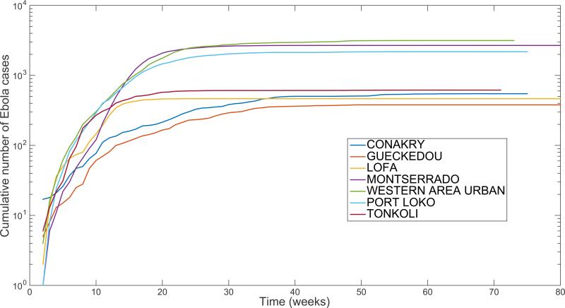
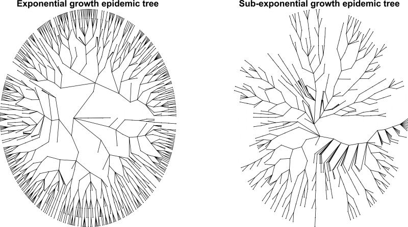
Because a necessary condition for validating a transmission model is that the model is able to reproduce growth patterns that are consistent with observed epidemiological data, faithful characterization of the profile of early epidemic growth is a useful test of model accuracy. For instance, prior work has highlighted that the initial, seemingly exponential spread of the 2014-15 Ebola epidemic in West Africa at the national level was in fact a composition of local asynchronous and sub-exponential outbreaks [5,8]. That is, local district or county-level outbreaks of Ebola show spatial asynchrony and follow a slower growth pattern that can be best approximated by polynomial rather than exponential functions during at least 3 consecutive disease generations (Figure 1). To further illustrate this point using simulations, we visually contrast exponential vs. sub-exponential epidemic growth dynamics using two representative transmission trees over 12 generations of disease transmission (Figure 2).

Figure 1.

The district level curves of weekly Ebola case counts during the 2014 Ebola epidemic are largely characterized by sub-exponential growth during the early epidemic phase, shown by the strong curvature in the cumulative incidence curves in semi-logarithmic scale.

Figure 2.

Schematic epidemic trees characterized by exponential and sub-exponential growth dynamics with12 generations of disease transmission where the index case is located in the center. The epidemic tree with exponential growth dynamics was stochastically generated assuming a mean basic reproduction number of 1.5 in the absence of interventions or behavior changes. The epidemic trees with sub-exponential growth dynamics are characterized by an effective reproduction number that declines towards unity over subsequent generations.

Past research has also identified polynomial epidemic growth patterns for HIV/AIDS [9], a viral disease that is spread largely through close contact via bodily fluids [6,10]. In particular, it has been well documented that the cumulative number of AIDS cases in the United States in the 1980s followed polynomial rather than exponential growth in time [9,10]. On a semi-logarithmic scale, exponential growth patterns are visually evident if a straight line fits well several consecutive disease generations of the epidemic curve, whereas a strong downward curvature in semi-logarithmic scale is indicative of sub-exponential growth. In the following subsection, we review a quantitative framework to characterize the early ascending phase of infectious disease outbreaks from case incidence series, using a phenomenological model [7]:

$$\frac{dC\left(t\right)}{dt}=C^{\prime }\left(t\right)=rC{\left(t\right)}^p$$ (1)

where C'(t) describes the incidence curve over time t, the solution C(t) describes the cumulative number of cases at time t, r is a positive parameter denoting the growth rate and p∈ [0,1] is a “deceleration of growth” parameter. If p=0, this equation describes constant incidence over time and the cumulative number of cases grows linearly while p=1 models exponential growth dynamics (i.e., Malthus’ equation). Intermediate values of p between 0 and 1 describe sub-exponential (e.g. polynomial) growth patterns. For example, if p=1/2 incidence grows linearly while the cumulative number of cases follows a quadratic polynomial. For sub-exponential growth (i.e., 0<p<1) the solution of this equation is given by the following polynomial of degree m [11]:

$$C\left(t\right)={\left(\frac{r}{m}t+A\right)}^m$$ (2)

where m is a positive integer, and the “deceleration of growth” parameter is given by p=1-1/m. A is a constant that depends on the initial condition, C(0). Specifically, $\mathrm{A}=\sqrt[m]{C\left(0\right)}$. Furthermore, for sub-exponential growth dynamics, the per-case growth rate, [dC(t)/dt]/C(t ∝ m/t, decreases inversely with time while the doubling time increases proportionally with time T_d ∝ t(ln 2)/m increases proportionally with time (Figure 1)[5]. In contrast, exponential growth is characterized by constant doubling times.

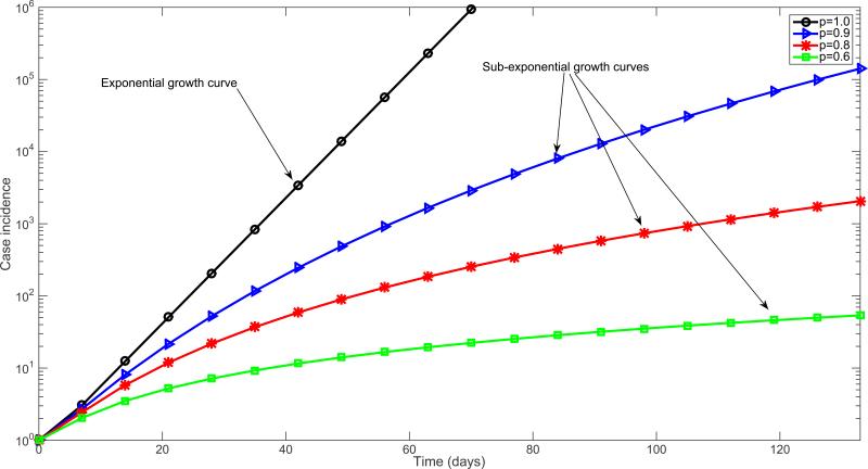
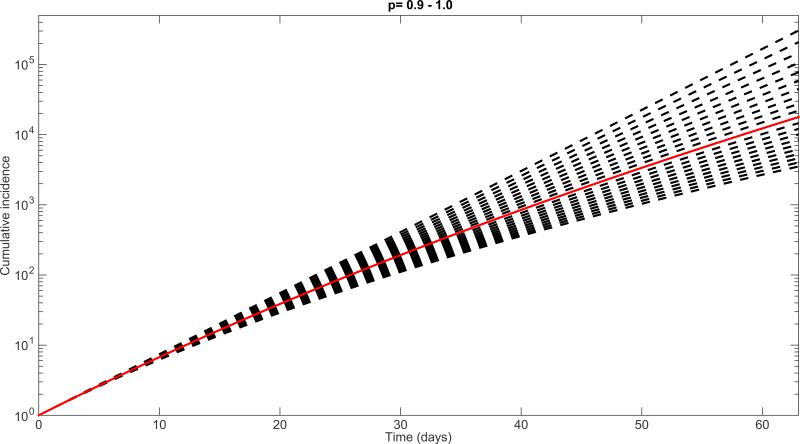
Simulations derived from the generalized-growth model display different epidemic growth profiles, as the “deceleration” parameter (p) is varied between zero and one (Figure 3). These profiles include linear incidence (i.e., p=0.5), concave-up incidence (p>0.5), and concave-down incidence (p<0.5) patterns. Moreover, epidemic size is predicted to be highly sensitive to small variations in the deceleration parameter p. This is highlighted in Figure 4 which displays an 86-fold difference in cumulative incidence between p=0.9 and p=1 (i.e., exponential growth) after 2 months with the growth rate parameter fixed at r=0.2 and C(0)=1.

Figure 3.

Simulated profiles of epidemic growth supported by the generalized growth model when varying the deceleration of growth parameter p (Equation 1) between 0 and 1. The growth rate parameter r is fixed at 0.2 per day and the initial number of cases, C(0)=1. In semi-logarithmic scale, exponential growth patterns are visually evident if a straight line fits well several consecutive disease generations of the epidemic curve, whereas a strong downward curvature in semi-logarithmic scale is indicative of sub-exponential growth.

Figure 4.

Simulations of epidemic growth profiles assessing the sensitivity of the cumulative number of cases to small variations in the deceleration of growth parameter p from p=0.9 to p=1.0 (i.e., exponential growth-dynamics) using the generalized-growth model (Equation 1) while fixing parameter r at 0.2 per day and C(0)=1. The solid red curve denotes the solution curve when p=0.95.

Phenomenological approaches for modeling disease spread are particularly suitable when significant uncertainty clouds the epidemiology of an infectious disease including the potential contribution of multiple transmission pathways [12]. In these situations, phenomenological models provide a starting point for generating early estimates of the transmission potential and generating short-term forecasts of epidemic trajectory and predictions of the final epidemic size [12].

2.3. Epidemic growth profiles in infectious disease outbreak data

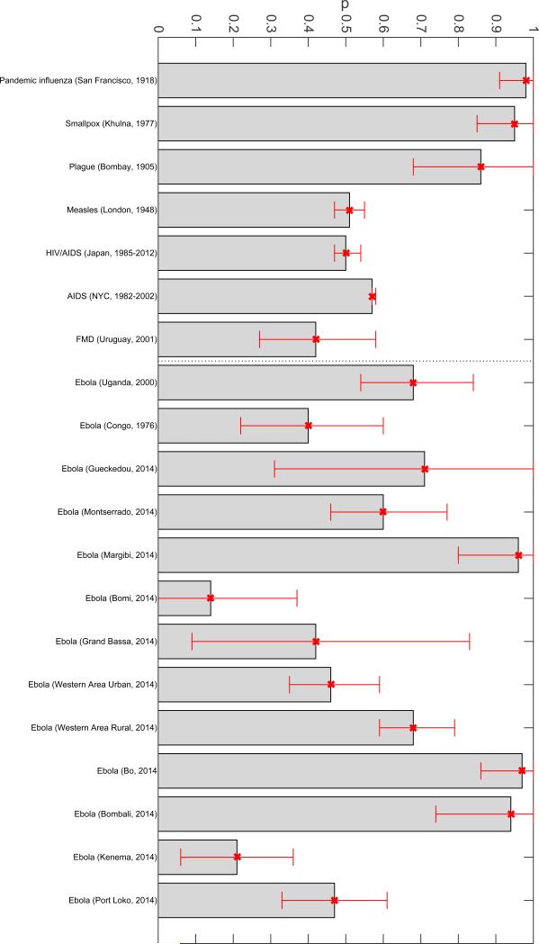
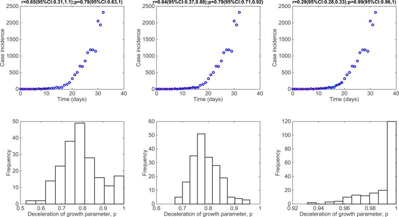
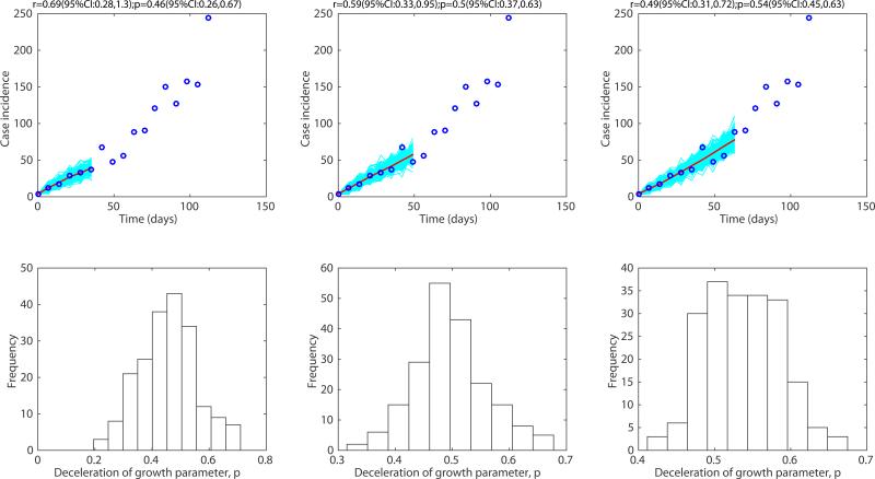
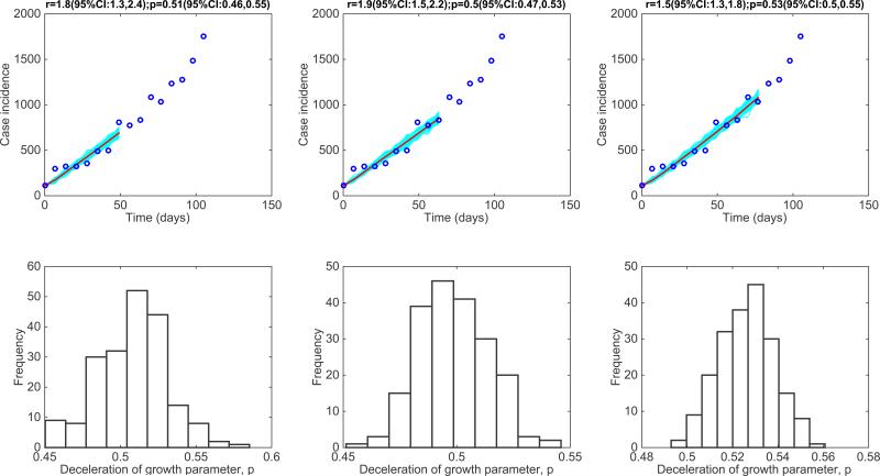
Previous work has shown that sub-exponential growth dynamics was a common phenomenon across a range of pathogens, as illustrated by empirical data on the first 3-5 generations of epidemics of influenza, Ebola, foot-and-mouth disease, HIV/AIDS, plague, measles and smallpox [7] (Figure 5). Representative fits of the generalized growth model to outbreak data and the corresponding empirical distributions of the deceleration of growth parameter p are shown in Figures 6-9. For instance, high values of p above 0.85 were estimated for a major plague epidemic in Bombay in 1905, the 1918 influenza pandemic in San Francisco, and a smallpox outbreak in Khulna, Bangladesh in 1972. Slower growth profiles were quantified for the foot-and-mouth disease outbreak in Uruguay at the farm level with a low mean estimate of p at 0.4 and the HIV/AIDS epidemic in Japan (1985-2012) at ~0.5, which is consistent with an approximately linear growth pattern [7].

Figure 5.

Estimates of p and corresponding 95% confidence intervals derived from various infectious disease outbreaks for a range of diseases including influenza, Ebola, foot-and-mouth disease, HIV/AIDS, plague, measles and smallpox [7]. The vertical dashed line separates Ebola and non-Ebola outbreak estimates.

Figure 6. The 1918 influenza pandemic in San Francisco, California.

Representative fits of the generalized-growth model (Equation 1) to an increasing amount of case incidence data during the initial epidemic growth phase (top panels) and the corresponding empirical distribution of the deceleration of growth parameter, p (bottom panel).

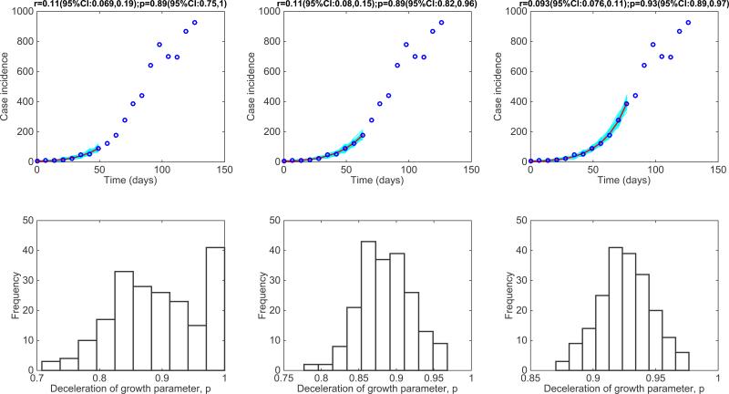
Figure 9. The 2014 Ebola epidemic in Western Area Urban, Sierra Leone.

Representative fits of the generalized-growth model (Equation 1) to an increasing amount of case incidence data during the initial epidemic growth phase (top panels) and the corresponding empirical distribution of the deceleration of growth parameter, p (bottom panel).

For the district-level Ebola epidemic outbreaks in West Africa, we found that p varied substantially with an overall mean at ~0.6 [7]. The districts of Margibi in Liberia, and Bombali and Bo in Sierra Leone, displayed near exponential growth (p close to 1), while the districts of Bomi in Liberia and Kenema in Sierra Leone displayed particularly slow growth (p near 0.1). An intermediate pattern of growth for the district of Western Area Urban in Sierra Leone is shown in Figure 9. Recently, we have also characterized the early growth dynamics of the mosquito-borne Zika epidemic in Antioquia, Colombia, which displayed sub-exponential growth dynamics, with p estimated in the range 0.44 – 0.65[12]. This epidemic growth profile is likely shaped by substantial spatial heterogeneity in the transmission rate, which is significantly associated with heterogeneities in the vector population [12].

2.4. Implications of early sub-exponential growth patterns in infectious disease data

The diversity of epidemic growth profiles observed in real epidemic outbreaks underscores the importance of understanding the underlying mechanisms and their ramifications in the design of epidemic models, and how they affect estimation of key epidemiological parameters and forecasting accuracy. For instance, it is common practice to rely on mechanistic epidemic models largely based on homogenous mixing assumptions, whereby the initial growth phase is assumed to follow an exponential growth phase during several generations of the disease (e.g. [1,13,14]). This suggests that predictions of final epidemic size based on models that assume early exponential growth will tend to overestimate epidemic size whenever the early dynamics of disease transmission are governed by mechanisms that induce slower transmission patterns. In turn, public health authorities could have more time to implement effective control interventions than forecasted. For instance, the predictions of the expected number of cases of HIV/AIDS in the United States or Ebola in West Africa that relied on models based on exponential growth assumptions greatly overestimated the final epidemic size [15-19].

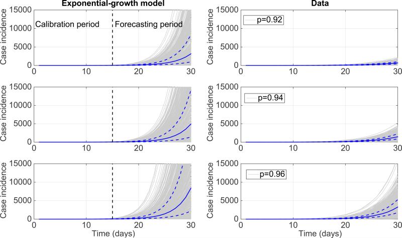
It is often taken for granted that the early growth phase of most biological processes follows exponential growth dynamics. In the context of infectious disease spread, this assumption is often convenient to describe a transmission process with mass action kinetics using differential equations. The impact of assuming exponential growth on short-term epidemic forecasts is illustrated in Figure 10, when the underlying growth process is slightly slower than exponential. That is, we first calibrated the exponential growth model to the first 3 generations of disease transmission for each of 500 stochastic simulations of early growth disease transmission derived using the generalized-growth model (Equation 1) where each disease generation is fixed at 5 days, the ‘deceleration of growth’ parameter p is set at values 0.92, 0.94, and 0.96, just below the exponential growth regime at 1.0 while the true growth rate parameter is set at 0.4 per day. Using the calibrated exponential growth model, we forecasted epidemic growth for the following 3 disease generations for each epidemic realization. These results shown in Figure 10 illustrate how rapidly the epidemic forecasts diverge within just a few generations of disease transmission even when the “true” growth dynamics fall only slightly below the exponential growth regime.

Figure 10.

The impact of assuming exponential growth dynamics when forecasting a near-exponential epidemic growth phase. We first calibrated the exponential growth model to the first 3 generations of disease transmission from 500 stochastic simulations of early growth disease transmission derived using the generalized-growth model where each disease generation is fixed at 5 days, the ‘deceleration of growth’ parameter p (Equation 1) is set at 0.92, 0.94, and 0.96, just slightly below exponential growth, the true growth rate parameter is set at 0.4 per day, and C(0)=1. Next, using the calibrated exponential model for each of the stochastic simulations, we forecasted epidemic growth for the following 3 disease generations for each epidemic realization. The gray curves correspond to the ensemble of epidemic forecasts. The red solid and dashed lines correspond to the median and interquartile range computed from the ensemble of stochastic realizations, respectively. The vertical dashed line separates the model calibration period from the forecasting horizon. The stochastic simulations derived from the “true model” using the generalized-growth equation are shown for reference.

Overall, there is a need to consider sub-exponential growth patterns in the design and parameterization of mathematical transmission models. Indeed, past modeling efforts have incorporated mechanisms to account for slower than exponential growth patterns including models that gradually mitigate the transmission rate over time [20-23] or incorporate phenomenological parameters to capture non-homogeneous population mixing [24,25] and models with particular spatial network structures [26-34]. Designing mathematical models and statistical approaches that more flexibly capture the profile of epidemic growth could lead to enhanced model fit, improved estimates of key transmission parameters, and more realistic epidemic forecasts [12].

The presence of early sub-exponential growth patterns have direct bearing on the definition, estimation and interpretation of the basic reproduction number R₀, a key quantity for disease control [35]. R₀ is a dimensionless quantity that captures the average number of secondary cases generated by a primary infectious individual in a completely susceptible population. If the case incidence curve follows an early exponential growth phase during the first few disease generations, R₀ is expected to remain invariant during the first few disease generations in the absence of susceptible depletion, control interventions or reactive population behavior changes. That is, the effective reproduction number, R_t ≈ R₀ during the early growth dynamics of an epidemic. Yet, empirical observations indicate that 1) the duration of most epidemics, particularly those of rapid dissemination such as influenza and childhood infectious diseases, typically only last for a few disease cycles, and 2) epidemics with an early sub-exponential growth phase are common [7]. In the context of sub-exponential growth dynamics, even with small deviations from the exponential growth assumption, the reproduction number is not invariant during the first few generations of disease transmission, but is a dynamic quantity that declines over time towards 1.0 [35]. In the context of the generalized-growth model [7], the actual profile of the effective reproduction number is shaped by the ‘deceleration of growth’ parameter, p [7]. This highlights the fact that R₀ alone could provide limited information about the transmission potential of infectious disease [36-38]. Further theoretical work is needed to connect sub-exponential growth patterns into classic theoretical results of epidemic theory stemming from decades-old pioneering work including that of Ross [3] and Kermack and McKendrick [4].

3. Mechanistic models representing epidemic growth profiles

In this section, we reflect on several mechanisms that have been put forward to explain the sub-exponential epidemic growth patterns evidenced from infectious disease outbreak data [5-7]. These include spatially constrained contact structures shaped by the epidemiological characteristics of the disease (i.e., airborne vs. close contact transmission model), the rapid onset of population behavior changes, and the potential role of individual heterogeneity in susceptibility and infectivity.

Although attractive to provide a quantitative description of growth profiles, the generalized-growth model described earlier is a phenomenological approach, and hence cannot be used to evaluate which of the proposed mechanisms might be responsible for the empirical patterns. Explicit mechanisms can be incorporated into mathematical models for infectious disease transmission, however, and tested in a formal way. Identification and analysis of the impacts of these factors can lead ultimately to the development of more effective and targeted control strategies. Thus, although the phenomenological approaches above can tell us a lot about the nature of epidemic patterns early in an outbreak, when used in conjunction with well-posed mechanistic models, researchers can learn not only what the patterns are, but why they might be occurring.

In the following sections, we describe a series of mechanistic transmission models that are especially useful for understanding the early spread of an epidemic. In particular, we center our review on structured epidemic modeling approaches, including population-level spatial metapopulation models, and individual-based network and agent-based approaches. Our goal is to describe the basic structure of these types of models and then discuss the epidemic growth profiles that these approaches support. We also discuss two modifications of the standard SIR epidemic model that support early sub-exponential growth dynamics: 1) an SIR model that incorporates reactive behavior changes by modeling a time-dependent transmission rate, and 2) an SIR model that incorporates inhomogeneous mixing through a power-law scaling parameter.

Epidemic transmission models by their very nature focus on the spread of an infectious disease through a population, but this spread can be modeled in two fundamentally different ways: by looking at the entire population as a single group or set of linked subgroups (population-based) or by explicitly considering each individual that makes up the population and how interactions between unique individuals facilitate disease spread (individual-based). In population-based models it is generally assumed that differences among individuals within each modeled group or subgroup in risks for disease or other characteristics are negligible so that everyone can be treated as if they were identical, i.e., that the groups being modeled are homogeneous. It is important to note, though, that heterogeneity among a larger population can be included in models using a population-based framework by dividing the large population into groups that reflect specified types of heterogeneity (e.g., age groups, neighborhoods, behavioral risk groups, etc.). Individual-based models consist of groups of discrete individuals and model the specific interactions between the individuals. Such models usually assume substantial heterogeneity in risks and behaviors among individuals.

The SIR model and derivatives is the framework of choice to capture population-level processes. The basic SIR model, like many other epidemiological models, begins with an assumption that individuals form a single large population and that they all mix randomly with one another [1,4,39]. This assumption leads to early exponential growth dynamics in the absence of control interventions and susceptible depletion and greatly simplifies mathematical analysis (note, though, that other assumptions and models can also result in exponential growth). The SIR model is often not a realistic representation of the human behavior driving an epidemic, however. Even in very large populations, individuals do not mix randomly with one another—they have more interactions with family members, friends, and coworkers than with people they do not know. This issue becomes especially important when considering the spread of infectious diseases across a geographic space, because geographic separation inherently results in nonrandom interactions, with more frequent contact between individuals who are located near each other than between those who are further apart. It is important to realize, however, that there are many other dimensions besides geographic space that lead to nonrandom interactions among individuals. For example, populations can be structured into age, ethnic, religious, kin, or risk groups. These dimensions are, however, aspects of some sort of space (e.g., behavioral, demographic, or social space), and they can almost always be modeled in similar fashion to geographic space (see, for example, [40,41]).

The means by which a population is structured is of critical importance, because this issue essentially determines how and when susceptible and infectious individuals come into contact with each other and potentially pass on a disease. The earliest structured population models in epidemiology date to at least the 1940s [42] and 1950s [43], but the number of studies centering on the development and/or analysis of such models has exploded since the late 20^th century, and it is now routine for such models to be used for human diseases. Models of the spread of infectious diseases in a spatial or social context have been formulated at both the population- and individual-level. Population-level models can be further subdivided into metapopulation models, which include discrete, identifiable subpopulations, and spatially continuous models, which assume that a population is continuously distributed across space. Individual-level models are often represented as network models, which summarize disease-causing interactions at the individual scale. In the next section we discuss metapopulation epidemic models in more detail; individual-level models will be discussed subsequently.

3.1 Metapopulation spatial models

Metapopulation formulations are used for the vast majority of population-based models that consider the spatial spread of human infectious diseases and that address important public health concerns rather than theoretical model behavior. Consequently, our review of population-based models in this paper will be limited to a description of the metapopulation approach. Readers interested in more details on spatially continuous epidemiological models are encouraged to consult Sattenspiel [44] or Keeling and Rohani [45]. Metapopulation models themselves can be considered as networks with the groups represented by nodes and the interactions among groups represented as the network links [41].

Incorporating population structure into epidemiological models introduces complications that are not to be taken lightly, however. Population structure adds significant complexity to a model, with corresponding increases in the difficulty of mathematical analyses. For this reason, individual-based computer simulation models are being used more frequently to address the consequence of population and individual heterogeneity. In addition to the difficulties with model analysis, structured models generally require much more extensive and complex sorts of data in order to estimate their parameters, which increase by n times compared to equivalent single population models (n is the number of subpopulations being modeled). In spite of these complications, metapopulation models are still the most common type of model used to explore mathematically how diseases spread across space.

The n subpopulations being modeled using a metapopulation approach are assumed to be discrete groups that are linked together in some way. Usually the individual groups or subpopulations are considered to be well mixed and homogeneous; some sort of coupling mechanism then links groups to one another. The coupling mechanism, which, in spatial models, usually assumes movement of individuals between groups, is what allows an infection to spread from one group to another. However, the actual movement process may be either explicit or implicit, leading to the development of two general classes of spatial metapopulation models: a) cross-coupled models, and b) mobility models [44]. Cross-coupled models generally make use of mathematical structures that simplify the analysis, and in addition, the strength of the interactions (i.e., coupling) between groups is determined by the modeler and explicitly built into the structure of the model. In mobility models, the modeler specifies the rates of travel or mixing between groups, and the strength of the interactions between groups is an outcome of the mixing process among all subpopulations. Because of their greater ease of analysis and less intensive data requirements, until very recently cross-coupled models were more commonly used, but better availability of the data necessary for parameter estimation has resulted in an increasing number of new models that make use of the mobility approach (e.g. [46-54]).

3.1.1 Cross-coupled metapopulation models

Cross-coupled metapopulation models, which have been in use since at least the mid-1940s (early examples include [42,43,55]) do not model the process that brings individuals from different groups into contact with one another; rather, they incorporate a contact matrix that represents the strength or sum total of those contacts only. This contact matrix is sometimes referred to as the WAIFW, or “who acquires infection from whom” matrix. In the simplest cross-coupled models, the elements of this matrix represent both the influence of interactions between any two subpopulations and the risk of transmission as a consequence of those interactions; often, however, the transmission parameter is considered separately.

Using the SIR framework described above, a simple deterministic cross-coupled epidemic model can be written as follows:

$$\begin{array}{cc}\hfill \frac{d{S}_i}{dt}& =\mu N_i-\mu S_i-S_i\sum _{j=1}^n\frac{{\varphi }_{ij}{I}_j}{N_i}\hfill \\ \hfill \frac{d{I}_i}{dt}& =S_i\sum _{j=1}^n\frac{{\varphi }_{ij}{I}_j}{N_i}-(\mu +\gamma )I_i\hfill \\ \hfill \frac{d{R}_i}{dt}& =\gamma I_i-\mu R_i\hfill \end{array}$$ (3)

where S_i, I_i, and R_i are the numbers of susceptible, infectious, and recovered individuals, respectively, N_i is the total population size in subpopulation i, γ is the recovery rate, and μ is the rate of birth (and death) under the assumption of a non-growing population (total births = total deaths). ϕ_ij is the rate of effective contact between subpopulation i and subpopulation j; the set of ϕ_ij forms the elements of the WAIFW matrix. Note that in this formulation, the ϕ_ij implicitly include both the rate of contact and the probability of transmission.

In a metapopulation consisting of n distinct subpopulations, the WAIFW matrix can have up to n² nonzero elements, and sufficient data may not be available to estimate all the parameters. In addition, mathematical analysis may be difficult. Consequently, simplified mixing patterns are often used in such models. Common assumptions are that the contact patterns are symmetric, that between-group contact is less frequent than within-group contact, or that contact between groups is a function of the distance separating them and/or their relevant sizes.

3.1.2. Mobility metapopulation models

Like cross-coupled metapopulation models, mobility metapopulation models incorporate into their structure a matrix to represent the interaction between different groups, but they are mechanistically oriented and do this by considering the actual process by which such interactions occur. Transmission of the pathogen occurs within subpopulations, but the composition of those subpopulations explicitly includes not only residents of the subpopulation, but visitors from other groups.

The majority of mobility metapopulation models that have been developed for human diseases consider short-term or temporary mobility, because the time scale of the disease transmission process is such that long-term or permanent migration can be ignored. The mechanisms that need to be modeled for all time scales are similar, however, and the appropriate time scale to use in the mobility component is disease- and question-specific. We limit our discussion here to short-term human mobility.

In general, the mobility process that links the subpopulations of a metapopulation can be specified by explicitly considering the rates of movement both from one group to another and in the opposite direction. This process can also be modeled by considering first the rates at which individuals leave groups to visit other locations and then the possible destinations and average durations of those trips [56]. As in the cross-coupled models, incorporation of the spatial dimension and the mobility matrix to represent contacts between groups requires the addition of at least n² new parameters in the model. Consequently, many mobility models also use simplified matrices to represent the mobility. In recent years, however, a number of new and detailed data sources that provide the information needed to specify these matrices have become available, increasing the feasibility and use of mobility metapopulation models. Examples of these are discussed further below.

An example of a deterministic SIR mobility metapopulation model is the following set of equations:

$$\begin{array}{cc}\hfill \frac{d{S}_i}{dt}& =\mu N_i-\frac{{\beta }_i{S}_i{I}_i}{N_i}-\mu S_i+\sum _{j=1}^n{\theta }_{ij}{S}_j\hfill \\ \hfill \frac{d{I}_i}{dt}& =\frac{{\beta }_i{S}_i{I}_i}{N_i}-(\mu +\gamma )I_i+\sum _{j=1}^n{\theta }_{ij}{I}_j\hfill \\ \hfill \frac{d{R}_i}{dt}& =\gamma I_i-\mu R_i+\sum _{j=1}^n{\theta }_{ij}{R}_i\hfill \end{array}$$ (4)

where S_i, I_i, and R_i are the numbers of susceptible, infectious, and recovered individuals, respectively, and N_i is the total population size of subpopulation i, μ is the rate of birth (and death) under the assumption of a non-growing population (total births = total deaths), ß_i is the transmission parameter in subpopulation i, and θ_ij is the rate of movement to subpopulation i from subpopulation j. In this simple model the rates of movement are assumed to be the same for all disease states, although this assumption can be relaxed if desired. Relaxation of the assumption does increase the data requirements for parameter estimation as well as the complexity of any model analyses, however.

Because mobility metapopulation models explicitly incorporate the movement of individuals between groups, the individuals making up a group can only be in one group at a time (i.e., they are either at home or they are visiting some other group). This means that they cannot be involved simultaneously in two different epidemic processes—their risk of transmission is a function only of where they are situated at the time transmission occurs. Depending on how the contact matrix is defined, however, this may not be the case for a cross-coupled model, although this problem can be offset by proper scaling of the transmission parameters [44].

3.1.3. Patterns of contact between groups in spatial metapopulation models

The defining characteristic of spatial metapopulation models is the contact matrix or set of between-group travel rates that determines the frequency of contact and opportunities for interaction between groups. In this section we provide an overview of the types of mixing/coupling patterns that are most prevalent in spatial metapopulation models, including both theoretical patterns and those that are derived from data such as airline travel or mobile phone usage. We also briefly examine recent research on determining the nature of contemporary human mobility.

Both cross-coupled and mobility metapopulation models developed in recent years represent the contact or mobility process by a matrix with parameters derived either from one of two generalized models, the gravity or radiation models, or from data that provide information on actual patterns of interaction within and among groups. The gravity model assumes that the rate of contact between two groups is directly proportional to their sizes and inversely proportional to the geographic distance separating them[57-59]. A generalized gravity model takes the form

$$m_{jk}=\frac{N_j^a{N}_k^b}{d_{jk}^c}$$

where m_jk represents the contact between groups j and k, N_j and N_k are the population sizes of the groups, d_jk is the distance between the two groups, and a, b, and c are parameters derived from fitting the model to existing data on interactions between the groups.

Because the data needed to parameterize the gravity model are often not available for regions without regular collection of traffic data, Simini et al. [60] recently proposed a new model, which they call the radiation model. Their model is intended to represent commuting behavior, and they assume that the destinations are determined only by job selection, which is a decision that depends on the size of the location of a specific job opportunity as well as the benefits (e.g., income, working hours, conditions, and other characteristics) of the potential opportunity.

Individuals choose the closest job to their home region that has higher benefits than those within the home region. The assigned work locations of all members of a region determine the daily commuter fluxes. The average flux, T_ij, from region i to region j at a distance r_ij apart is given by

$$\langle T_{ij}\rangle =T_i\frac{N_i{N}_j}{(N_i+s_{ij})(N_i+N_j+s_{ij})}$$

where N_i and N_j are the population sizes of regions i and j, respectively and s_ij is the total population in a circle of radius r_ij centered on region i but excluding both the source and destination populations. $T_i={\sum }_{j\ne i}{T}_{ij}$ is the total number of commuters who begin their commute in region i. Simini et al. [60] show that the commuting fluxes, T_ij, are independent of the benefits distribution as well as the density of jobs, and the total number of commuters, the remaining free parameter, also does not affect the distribution of the T_ij; consequently, their model is parameter-free. All that is required as input for the model is the population distribution, which is almost always available throughout the world.

The other approach to estimating the contact matrix linking different subpopulations in a spatial metapopulation model is to use actual data that provide direct information on individual movement patterns, and this approach is becoming more and more widespread. A number of large-scale data sets are available from many parts of the world, with the most common sources being mass transportation (e.g., airline, rail, bus) data and mobile phone data. For example, Tizzoni et al. [61] compared the ability of different types of data to effectively represent commuting networks at different spatial scales. They focused on regularly collected census surveys, mobility phone data, and a radiation model calibrated using census data from three European countries—Portugal, Spain, and France. They incorporated the resulting contact matrices into metapopulation models for these countries and compared model results to observed epidemiological data. They found that mobile phone data effectively captured the commuting patterns and were highly correlated with the census-derived patterns, but that the data systematically overestimated the volume of commuting traffic and therefore predicted more rapid spread of epidemics.

3.1.4. Early epidemic growth dynamics from spatial metapopulation models

The use of different spatial structures in transmission models has proven useful to gain greater understanding of how population structures found in the real world may influence the speed of epidemic spread and the clustering of cases. The presence of spatial structure implies that individuals do not mix randomly with others throughout the population and as a consequence, disease cases are likely to show clustering rather than to diffuse smoothly across the space. This clustering can also reduce the speed of epidemic spread throughout the entire population. Recall, though, that a common assumption of spatial metapopulation models is that the subpopulations are homogeneous and randomly mixing. Thus, although epidemic spread throughout the entire population is generally slower in a metapopulation than in a comparably sized homogeneous population, analyses have shown that metapopulation models result in consistently faster spread and higher incidence than analogous individual-based models that do not assume homogeneous populations and random mixing within groups [62,63]. Even more relevant for this review is the fact that whenever the local (patch) population size is large enough in a metapopulation transmission model, case incidence is expected to follow exponential growth dynamics in the absence of control interventions or behavior changes and depletion of susceptibles. This indicates that metapopulation models may not explicitly provide the right spatial scale to capture specific spatial features (e.g., clustering), which could yield early sub-exponential growth dynamics.

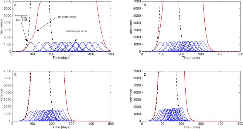
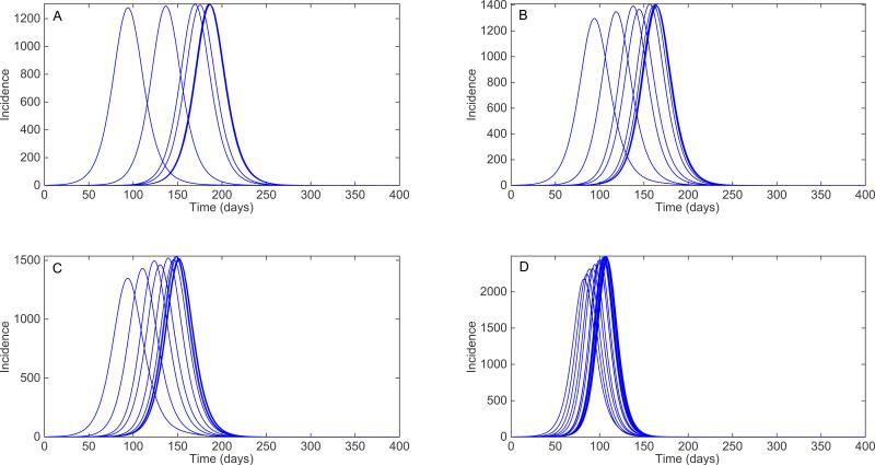
For illustration, Figure 11 displays the impact of increasing transmission rates of the 4-nearest neighbors on local epidemic simulations using a cross-coupled metapopulation model where 100 local populations each of size 100,000 are spatially arranged in a 10 × 10 square lattice structure. Perhaps not surprisingly, one can observe how the early local epidemic growth dynamics during the first few generation intervals corresponds well to the epidemic growth derived from a simple SEIR transmission model in a homogenously mixed population. By adding a hub population to this metapopulation structure (e.g., a small and constant transmission rate from all patches to/from a hub population; see e.g., [64,65]), the local epidemic dynamics across the population become increasingly synchronized as shown in Figure 12.

Figure 11.

Local epidemics generated using a cross-coupled metapopulation model where 100 local populations are spatially arranged in a 10 × 10 square lattice with periodic boundary conditions. The local dynamics across all patches follow a simple SEIR (susceptible-exposed-infectious-removed) transmission model with a mean latent period of 2 days, a mean infectious period of 3 days, a local basic reproduction number, R₀ at 1.5, and a local population size in each patch of 100,000 individuals. A constant transmission between the 4-nearest neighbors is modeled as a fraction ρ of the local transmission rate, which takes values of A) 0.1%, B) 0.5%, C) 1% and D) 5%. For reference, the red dotted line corresponds to the curve of total incidence while the dashed black line corresponds to the solution of the homogenous mixing SEIR model considering the total homogenously-mixed population in a single patch.

Figure 12.

Local epidemics generated using a cross-coupled metapopulation model where 100 local populations are spatially arranged in a 10 × 10 square lattice. The local dynamics across all patches follow a simple SEIR (susceptible-exposed-infectious-removed) transmission model with a mean latent period of 2 days, a mean infectious period of 3 days, a local basic reproduction number, R₀ at 1.5, and the local population size is 100,000 individuals. The nearest neighbor transmission rate is modeled as a fraction p of the local transmission rate, which takes values of A) 0.1%, B) 0.5%, C) 1% and D) 5%. In addition to nearest-neighbor transmission, transmission with a single hub population is possible with which all patches interact by modeling a hub-transmission rate which is assumed to be fixed at 1% of the nearest neighbor transmission rate.

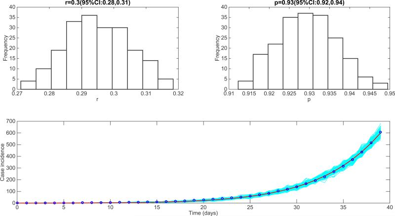
The Global Epidemic and Mobility (GLEaM) Model, a mobility metapopulation model that uses worldwide airline travel data and a gravity model to approximate the transportation network, has also been used to study early epidemic growth profiles [66-68]. The GLEaM transportation network is combined with a realistic population distribution to project the spatial spread of an epidemic. The model has been employed to address different policy questions including the potential role of travel restrictions. The early epidemic growth profile of 2009 A/H1N1 pandemic influenza was assessed using simulations derived from GLEaM. Specifically, the epidemic growth pattern was characterized from the incidence curve for Mexico City for the 2009 A/H1N1 influenza pandemic as obtained from GLEaM [66]. In line with our previous discussion about metapopulation models, using the generalized-growth model described in Section 2, we found exponential growth dynamics during the early phase of the 2009 A/H1N1 influenza pandemic in Mexico City as shown in Figure 13. These findings are in agreement with the early dynamics of pandemic influenza described in [7], which suggests that metapopulation models can provide the appropriate baseline spatial structure for modeling the spread and control of infectious diseases that disseminate rapidly, such as pandemic influenza or the spread of childhood infectious diseases in highly naïve populations.

Figure 13.

Characterization of the epidemic growth pattern from the incidence curve of the 2009 A/H1N1 influenza pandemic in Mexico City as provided by GLEAM [66]. Using the generalized-growth model described in Section 2, we found near-exponential growth dynamics during the early phase of the 2009 A/H1N1 influenza pandemic in Mexico City, which is in line with the early dynamics of pandemic influenza described in [7].

3.2. Individual-based network models

With the increasing availability of data, computational power and methodological advancements, the approaches of network models have been increasingly sought for problems of infectious disease dynamics (reviewed in [69-71]). A contact network model explicitly represents host interactions that mediate disease spread. A node in a contact network represents an individual host, and an edge between two nodes represents an interaction that may allow disease transmission. Network models can thus capture individual-scale variation in vulnerability to infection and potential for infecting others, which may be dictated by an individual's connectivity to other individuals in the network as well as individual susceptibility and infectivity.

Network-based epidemic modeling methods have the power to study the impact of individual-level characteristics and their disease-relevant interactions on the transmission dynamics observed at the population level. Several such methods, both simulation-based and analytical, have been developed in the last thirty years. Simulation methods include discrete-time and continuous-time models, and enable the study of complex network structures without approximation. When tractability is desired, analytical methods provide an alternative through numerical integration. For a comprehensive review of network epidemic modeling methods, we point the reader to [70].

While little work has explicitly addressed the early growth dynamics using contact network models, individual-based network models are amenable to studies of how specific structural features affect early epidemic growth patterns. In particular, individual-based networks are useful to capture two important mechanisms that are expected to slow down the initial growth dynamics: a) local susceptible depletion, in which the pool of susceptibles available to infectious individuals diminishes even at low rates of prevalence [71]; and b) risk heterogeneity, which segregates the population into high and low infection risk. Local susceptible depletion mitigates the initial growth rate by limiting local spread; and risk heterogeneity tends to focus early case growth to those at highest risk of infection. In the following subsections, we highlight three key network structural features (contact heterogeneity, clustering, and dynamic contacts) that play an important role in the transmission dynamics of disease spread, and are affected by both mechanisms discussed above. We also briefly review analytical network modeling approaches, including bond percolation, pair approximation, and dynamic networks, which are useful to analyze the impact of individual-based transmission processes on early epidemic growth dynamics. Our analysis of the literature on investigating the impact of individual-level transmission characteristics on early spread dynamics indicates a clear need for systematic studies that increase our understanding of the impact of different configurations of clustering, contact heterogeneity, and individual-level variation in susceptibility and infectivity on the early epidemic growth dynamics.

3.2.1 Contact heterogeneity

Variation in the number of contacts, or disease-causing interactions, among hosts in a population has been shown to impact disease outcomes and the design of intervention strategies [72-79]. In network terms, the degree of an individual (node) represents the number of contacts (edges) it has with other individuals, and the degree distribution represents the frequency distribution of node degrees. The degree distribution is a powerful way of characterizing a network as it naturally captures the individual-level heterogeneity in the potential to acquire infection from other individuals and to transmit infection to others. A parsimonious model of contact heterogeneity is the configuration model [80], which generates networks with a specified degree distribution that is random in all other respects. Volz and others developed an “edge-based compartmental modeling” (EBCM) formalism (based on probability generating functions) for dynamically modeling SIR-type epidemics on configuration model networks [81,82]; this was a significant improvement over existing bond percolation methods at the time [83]. This method provides a means of translating between population quantities (total number of contacts) and individual quantities (number of susceptible and infected individuals) to determine epidemic incidence at any time. This approach and others have been used to demonstrate the dramatic effects that the degree distribution can have on disease spread in a population: homogeneous populations (with low variance degree distributions) are characterized by a high epidemic threshold and experience a lag before reaching the expansion phase of the epidemic; heterogeneous populations (with high variance degree distributions) have low epidemic thresholds and accelerate very rapidly [69,75,79,81]. Nevertheless, as we elaborate below, the degree distribution of a contact network is only one of several network features that drive the transmission dynamics of an infectious disease, when spatial structure is relevant. Indeed, in a seminal paper, Watts and Strogatz (1998)[78] devised the “small-world” network model to demonstrate that networks with essentially the same degree distribution could give rise to completely different temporal epidemic profiles when individual nodes were connected in a spatially correlated manner.

The observed polynomial growth of the HIV/AIDS epidemic was first hypothesized to be the result of heterogeneity in the distribution of contacts such that models with extreme contact heterogeneity generated epidemics with slower than exponential growth owing to saturation among the highly connected classes of individuals, which led to a transition to less connected individuals [9]. In fact, Colgate et al. [10] demonstrated that it was likely substantial heterogeneity in contact frequency and a hierarchical spread through connectivity classes that led to the early cubic growth of AIDS in the United States. However, these findings were derived using compartmental models based on differential equations, and it would be very interesting to gain better understanding of these findings using network models guided by realistic sexual contact network datasets or realistic contact structures. Hence, the question: “Can disease spread on realistic individual-level sexual contact networks give rise to polynomial growth epidemics in the absence of control interventions or behavior changes?” is one that remains open.

Multiple factors could interact with the role of contact heterogeneity on disease spread particularly when the latter is correlated with other individual-level heterogeneities such as individual susceptibility and infectivity, both of which affect the transmission process. For instance, Smilkov et al. [84] apply a discrete-time SIS model on networks to investigate the role of susceptibility variation in relation to contact variation on the transmission dynamics. This is an important issue because variation in the susceptibility of individuals is a common phenomenon that can be the result of age, genetics, or socio-economic factors. They find that if there are individual-level correlations between the susceptibility and degree of a node, the early growth and persistence of an outbreak may be under- or overestimated.

3.2.2 Clustering & spatial structure

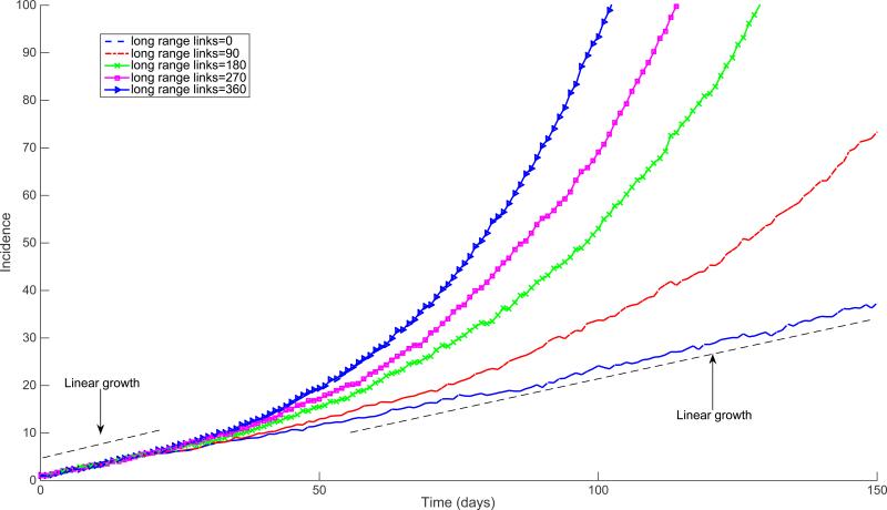
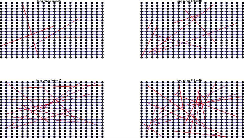
Empirical networks do not always satisfy the assumption of random or uncorrelated contacts made by the configuration model, as they are expected to have non-trivial structural properties including clustering and degree correlations [85]. Szendroi and Csanyi [6] proposed that polynomial growth in epidemics is driven by network clustering, a property of the contact network that quantifies the level of overlap between an individual's contacts and their contact's contacts. The small-world model [78] implemented in a 2D lattice with no random links gives rise to polynomial growth epidemics (Figure 14). Indeed, when high clustering is accompanied by long path lengths in lattice models, spatial saturation leads to asynchrony in infection dynamics, slowing down early growth [86]. However, Watts and Strogatz showed that the addition of very low levels of random contacts yields an overall transmission process that becomes very similar to that generated on random networks [78]. Here, we briefly examine via simulations the early growth dynamics of disease spread on small-world networks that include a slight amount of randomness (Figure 15). These results indicate that the average incidence on 2-dimensional small-world networks with small amounts of randomness can yield polynomial growth during the first few transmission cycles. However, case incidence accelerates as the infection reaches distant population segments through the long-range random links. Indeed, when high clustering is accompanied by long path length, as in lattice models and small world networks with few long range edges, spatial saturation leads to asynchrony in infection dynamics, slowing down early growth [86].

Figure 14.

Early epidemic growth profiles simulated using the SIR (susceptible-infectious-recovered) model on a 2D square lattice with dimensions 90 × 90 (90,000 individuals) with periodic boundary conditions. The mean of 200 stochastic simulations is shown for lattices with an increasing number of long-range random links as a function of the total population size (0%, 0.1%, 0.2%, 0.3%, 0.4%, 0.5%).

Figure 15.

Schematic representation of 2D square lattices where each node is connected to its 4-nearest neighbors with periodic boundary conditions and with the addition of a few random long-range links.

The role of clustering at the population level has also been studied through pairwise approximation models. Pairwise approximation (PA) models offer a parsimonious means of extending mean-field models to incorporate network structure between hosts by tracking the density of pairs of individuals (e.g. susceptible-susceptible, susceptible-infected, etc.) rather than single individuals (susceptible, infected, etc.)[87]. Although more complex versions of the pairwise approximation model have been developed to deal with contact heterogeneity [88], the simple model particularly captures (low levels of) clustering by approximating the number of triples (e.g. susceptible-susceptible-infected) in terms of the number of pairs[87]. Studies that have investigated epidemic dynamics using pair approximation models include those of Keeling[89] and Eames [90]. Because pair-approximation models rely on mass-action mixing as a building block, the early epidemic spread stemming from this type of models is exponential. However, Dangerfield et al [91] also demonstrate that stochastic pair approximation models show increased variance in early growth dynamics when compared to deterministic mean field models.

3.2.3 Dynamic contacts

Social contacts are neither continuous nor permanent. Various forms of network dynamics are known to be relevant to disease dynamics including school terms, changes in sexual relationships, and host mobility, as well as behavioral changes driven by disease and intervention (e.g., social distancing and school closure) [92]. Traditional static network models predict a direct relationship between the probability of transmission between individuals and the growth rate of an outbreak. The results of Volz and Meyers [93], however, suggest that the evolution of network structure can produce more complex patterns of disease spread. In particular, they extend the EBCM formalism described above to include contact turnover at a specified rate (assumed to be 1 in mean-field models), and show that contact turnover results in reduced epidemic growth.

Several other studies have also investigated the impacts of such temporal features on epidemiological processes. The work of Smieszek et al. [94] and Eames [90] suggests that higher frequencies of repeated contacts reduces epidemic growth, and that this effect is stronger with low numbers of contacts or a low transmission probability. Using an empirical data set of physical contacts, Read et al. [95] demonstrated that both high regularity and duration of contacts have the same effect. On the other hand, high concurrency of contacts, which has been studied intensely in the context of sexually transmitted infections, leads to faster-growing outbreaks and larger final epidemic sizes [96].

The impact of network evolution through behavioral changes has also been studied recently using a network approach. Using SIS and SIR epidemic models on configuration model networks, Britton et al. [97] studied the impact of social distancing on the early stages of an outbreak. In particular, they considered preventive rewiring, in which susceptible individuals break off contacts with infectious individuals at a specified rate and replace those contacts with non-infectious individuals. Britton et al. found that preventive rewiring decreases the initial rate of growth as long as only susceptible individuals engage in this behavior (preventive rewiring by exposed individuals increases growth and is more harmful in the long term).

3.3 Examining early growth from spatial models

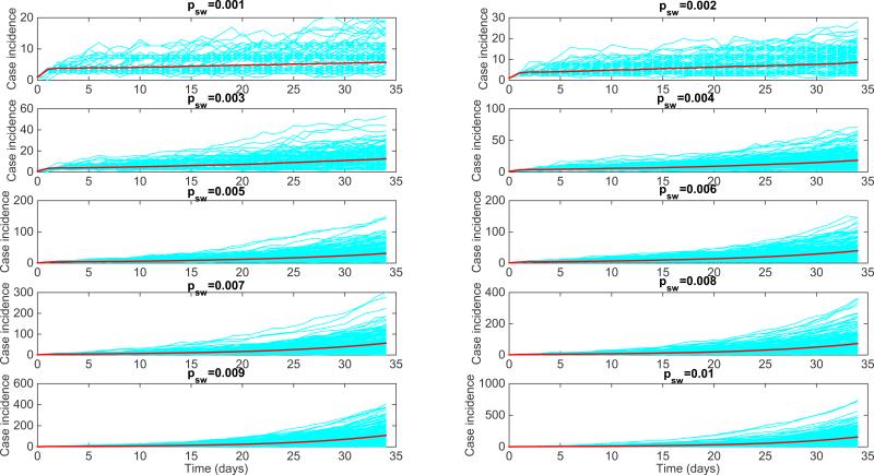
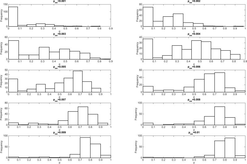
In this section, we illustrate how the generalized-growth model reviewed in Section 2 can be used to gain a better understanding of the dynamics of early epidemic growth arising from simulations of disease transmission on individual-level network models with varying levels of complexity. Specifically, we simulated SIR (susceptible-infectious-removed) dynamics on small-world networks using networks of size N=90,000 and node connectivity to the 4 nearest neighbors, and we increased the edge rewiring probability parameter (p_sw) from 0.001 to 0.01 of the small-world network model of Watts and Strogatz [78]. For each value of p_sw, we analyzed the early epidemic growth profile comprising 35 days of disease transmission from 200 stochastic realizations. The transmission rate per contact per unit of time b was set at 2 and the infectious period ($\frac{1}{\gamma }$) was assumed to be exponentially distributed with a mean of 3 days. Each simulation started with one infectious individual selected at random from the network. For reference, the baseline SIR transmission dynamics on the regular network with node connectivity to the 4 nearest neighbors and without long-range links correspond to a wave of steady case incidence at about 4 cases per day. To assess the early epidemic growth profile, we estimated the deceleration of growth parameter p and the growth rate r of the generalized-growth model [7] during the early epidemic growth phase for each of the 200 stochastic realizations as in prior studies [7]. The corresponding simulations of the early epidemic growth in the small-world network model are shown in Figure 16. Interestingly, we found that the deceleration of growth parameter displays a bimodal distribution for low values of the rewiring edge probability (0.001-0.006) with many stochastic curves characterized by almost constant incidence (Figure 17). The bimodal shape vanishes as the edge rewiring probability approaches 0.01 (1% of the network edges are rewired at random according to the Watts-Strogatz network model), with the early growth dynamics in the small-world network model quickly approaching the exponential growth regime as p_sw increases.

Figure 16.

SIR-type early growth simulations on small-world networks constructed using the Watts-Strogatz model in ref. [78] with a low edge rewiring probability parameter (p_sw) varying from 0.001 to 0.01. The baseline SIR early transmission dynamics on the regular network with node connectivity to the 4 nearest neighbors and without long-range links correspond to a wave of steady disease spread at about 4 cases per day.

Figure 17.

Estimation of the deceleration of growth parameter (Equation 1) from the early growth phase of SIR simulations on small-world networks with varying edge rewiring probability ranging from 0.001 to 0.01. Findings indicate that the deceleration of growth parameter displays a bimodal distribution for the low values of the rewiring edge probability (0.001-0.006) with many stochastic curves characterized by almost constant incidence. The bimodal shape vanishes as the edge rewiring probability approaches 0.01 (1% of the network edges are rewired at random according to the Watts-Strogatz network model). That is, the early growth dynamics in the small-world network model quickly approach the exponential growth regime as p_sw increases.

3.3.1 Early epidemic growth dynamics from agent-based Ebola transmission models

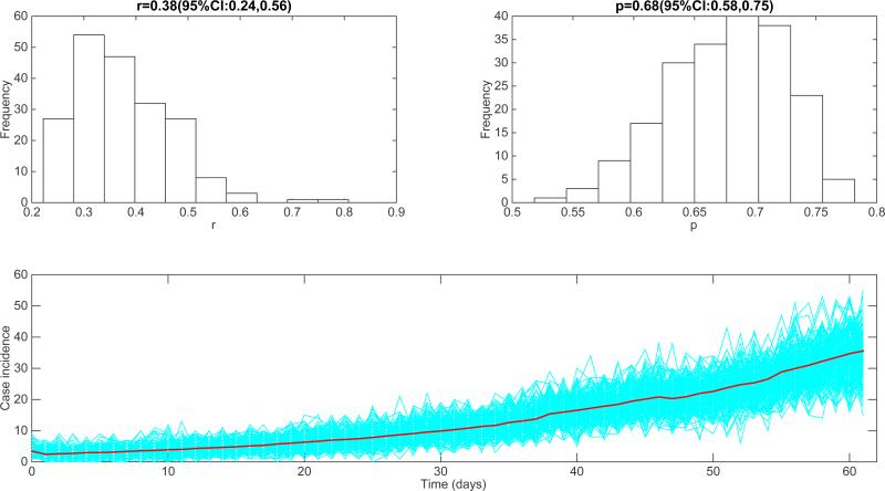
It is of interest to analyze the epidemic growth profile of epidemic simulations generated by realistic agent-based models specifically designed to study the transmission and control of infectious diseases. For diseases transmitted via close contact such as Ebola, one could expect sub-exponential growth dynamics during the early epidemic phase in the absence of control interventions or behavior changes and in line with observed epidemic patterns [5,7]. Here we used the generalized-growth model to quantify the epidemic growth profile stemming from individual-based transmission models previously designed to study the transmission dynamics of the 2014 Ebola epidemic in Liberia. We analyzed 200 stochastic simulations of the early epidemic growth phase derived from the individual-based Ebola model developed by Merler et al. [28]. Their model includes detailed geographic and demographic data from Liberia in order to model the mobility patterns of individuals in the population, which is structured into households based on Demographic Health Survey data. The model was calibrated to the situation in Liberia by estimating the proportion of transmission occurring in households, hospital settings, and via unsafe funerals [28]. Our analysis of the early epidemic growth phase using the generalized growth model is shown in Figure 18. We found a deceleration-of-growth parameter p at 0.68 (95% CI: 0.58, 0.75), indicating approximately cubic growth during the first 4-5 generations of disease transmission. Our results also demonstrate substantial variability in the epidemic growth profile across individual epidemic simulations as shown in Figure 18.

Figure 18.

Characterization of the early epidemic growth pattern from epidemic simulations derived by the detailed individual-level Ebola transmission model developed by Merler et al. [28]. We analyzed 200 stochastic simulations of the early epidemic growth. We found a deceleration of growth parameter p at 0.68 (95% CI: 0.58, 0.75), indicating approximately cubic growth during the first 4-5 generations of disease transmission.

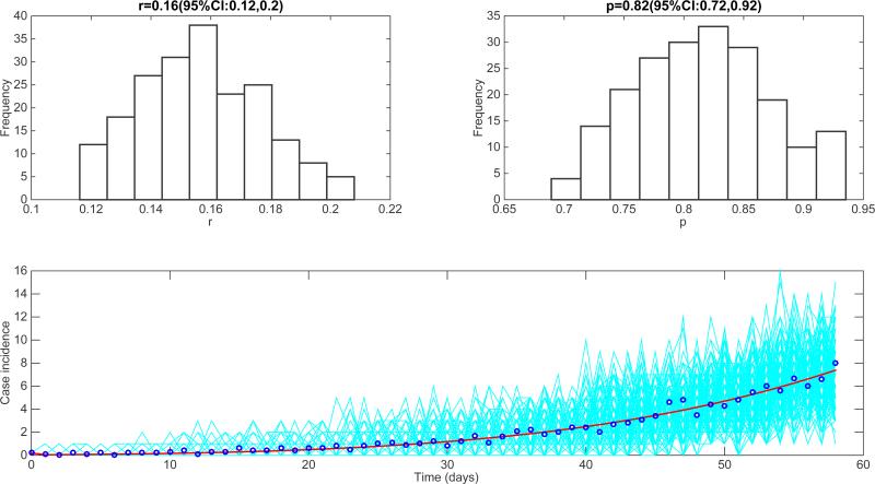
Another model that incorporated spatial features of the transmission dynamics of Ebola is that of Kiskowski [27]. This is a network-based SEIR transmission model with household-community structure, which was used to systematically analyze the effects of different levels of population mixing on Ebola transmission dynamics. The model was able to fit observed cumulative incidence curves by changing only the community mixing parameter [26,27], and it predicted that in the absence of epidemic control, persistent outbreaks would propagate through a community as spatial waves of fixed size [26]. Individuals are organized within households of size H (each household contains H individuals) and households are organized within communities of size C households (each community contains C×H individuals). Network connectivity is identical for every individual. Our analysis of the average epidemic curve generated by the model for the situation in Liberia is shown in Figure 19. We estimated the deceleration-of-growth parameter p at 0.82 (95% CI: 0.72,0.92), which is slightly higher than that obtained from the individual-based model of Merler et al. [28].

Figure 19.

Characterization of the epidemic growth pattern from the best fit of the spatial Ebola model of Kiskowski to the early phase of the Ebola epidemic in Liberia[27]. We estimated the deceleration of growth parameter p at 0.82 (95% CI: 0.72,0.92), which slightly higher than that obtained from the simulations derived from Merler et al's model.

3.4 SIR model with reactive behavior changes

Slower than exponential epidemic growth could also be explained by an increasing effect of population behavior changes and control interventions taking hold in the population during the early epidemic phase in such a way that the effective reproduction number declines and approaches 1.0. For instance, in the district of Gueckedou, Guinea associated with the epicenter of the 2014-15 Ebola epidemic, the rate of spread exhibited sub-exponential growth even before control interventions were put in place [5]. This supports the potential role of behavior changes and population structure on the early transmission dynamics of infectious diseases [5,98].

While previous efforts have reviewed transmission models that have incorporated the influence of human behavior on epidemic spread [99] and the challenges in incorporating the dynamics of behavior in infectious disease models [100], recent findings [5,7] support the need to develop modeling frameworks that account for the possibility of early sub-exponential growth dynamics to enhance our ability to forecast epidemics. For this purpose, we can build on the well-known SIR (susceptible-exposed-infectious-recovered) transmission model [1] by incorporating flexible early epidemic growth profiles, e.g., sub-exponential and exponential growth dynamics. This is achieved by allowing the effective reproduction number R_t to change dynamically in the context of early sub-exponential (e.g, polynomial) growth dynamics [35]. This approach is useful to describe a gradual effect of early behavior change that blunt the population transmission rate such that the reproduction number gradually declines towards the epidemic threshold at 1.0 [101].

The standard SIR (susceptible-infectious-removed) epidemic model [1,102] represents the simplest and most popular mechanistic compartmental model for describing the spread of an infectious agent in a well-mixed population. In this model, the force of infection per unit of time is simply given by the product of three quantities: the transmission rate β(t), and the probability that a susceptible individual encounters an infectious individual, which is given by $\frac{I\left(t\right)}{N}$. Moreover, infected individuals experience a mean infectious period given by 1/γ. The model is based on a system of ordinary differential equations that track the temporal progression in the number of susceptible, exposed, infectious, and removed individuals as follows:

$$\begin{array}{cc}\hfill \frac{dS\left(t\right)}{dt}& =-\beta \left(t\right)S\frac{I}{N}\hfill \\ \hfill \frac{dI\left(t\right)}{dt}& =\beta \left(t\right)S\frac{I}{N}-\gamma I\hfill \\ \hfill \frac{dR\left(t\right)}{dt}& =\gamma I\hfill \end{array}$$ (5)

In a completely susceptible population, e.g., S(0) ≈ N, the number of infectious individuals increases following an exponential function during the early epidemic growth phase, e.g., I(t) ≈ I₀e^(β–γ)t where the average number of secondary cases generated per primary case, R₀, is simply given by the product of the mean transmission rate (β) and the mean infectious period ($\frac{1}{\gamma }$) as follows:

$$R_0=\frac{\beta }{\gamma }$$

However, as the number of susceptible individuals in the population declines due to a growing number of infections, the effective reproduction number over time, R_t, is given by the product of R₀ and the proportion of susceptible individuals in the population:

$$R_t=\frac{S\left(t\right)}{N}\frac{\beta }{\gamma }$$

During the first few generations of disease transmission, in the absence of control interventions or reactive population behavior changes, the standard SIR model supports a reproduction number that is essentially invariant, e.g., R_t ≈ R₀. By contrast, in the context of epidemics characterized by early sub-exponential growth dynamics, the reproduction number is a dynamic quantity that declines over disease generations towards 1.0 [35]. We can incorporate the possibility of early sub-exponential growth dynamics by modeling explicitly the dynamic behavior of the reproduction number via a time-dependent transmission rate β(t) such that the force of infection becomes: β(t)S(t)I(t)/N. Specifically, we model an exponential decline in the transmission rate β(t) as follows:

$$\beta \left(t\right)={\beta }_0((1-\varphi )e^{-qt}+\varphi )$$

Thus, this time-dependent transmission rate β(t) allows the model to capture early sub-exponential growth dynamics whenever R₀ > 1 and q > 0. A special case is the standard SIR modeling framework when q = 0. The time-dependent transmission rate β(t) declines exponentially from an initial value β₀ towards ϕβ₀ at the rate q > 0. Assuming that R₀ > 1 and the population size N is sufficiently large such that the effect of susceptible depletion on the effective reproduction number due to new infections is negligible, the quantity(1–ϕ) models the proportionate reduction in β₀ that is needed to reach an effective stationary reproduction number of 1.0. Hence, ϕ can be simply estimated as $\frac{\gamma }{{\beta }_0}$. The decline rate parameter q can be interpreted through the half time value $\frac{log\left(2\right)}{q}$, the average time elapsed to achieve a transmission rate $\frac{{\beta }_0(1+\varphi )}{2}$. If q = 0, the transmission rate β(t) = β₀ remains at the baseline value, and we obtain the classic SIR transmission model with exponential growth dynamics and $R_0=\frac{{\beta }_0}{\gamma }$. In general, the higher the value of q, the faster the decline of the reproduction number from R₀ > 1 to a stationary reproduction number at 1.0. Importantly, in the context of early sub-exponential (e.g., polynomial) epidemic growth for which q > 0, the basic reproduction number R₀ is no longer the product of the initial transmission rate β₀ and the mean infectious period $\frac{1}{\gamma }$ because the transmission rate β(t) is no longer constant, but declines during the duration of the infectious period of primary cases at the onset of the epidemic, yielding a lower R₀ [103,104]. For this situation, R₀ can be estimated numerically using the following integral equation:

$$R_0={\int }_0^{\infty }\beta \left(\tau \right)e^{-\gamma \tau }d\tau ={\int }_0^{\infty }{\beta }_0((1-\varphi )e^{-q\tau }+\varphi )e^{-\gamma \tau }d\tau$$

For a given value of β₀ and γ, the basic reproduction number R₀ is expected to decline from $\frac{{\beta }_0}{\gamma }$ as parameter q increases above 0. More generally, the effective reproduction number, R_t, during the early epidemic growth phase comprising the first few disease generations of transmission when $\frac{S_t}{N}\approx 1$ can be numerically computed as follows:

$$R_t={\int }_t^{\infty }\beta \left(\tau \right)e^{-\gamma (\tau -t)}d\tau ={\int }_t^{\infty }{\beta }_0((1-\varphi )e^{-q\tau }+\varphi )e^{-\gamma (\tau -t)}d\tau$$

Using the above expressions, it is possible to estimate the basic reproduction number R₀ associated to the primary cases at the onset of the epidemic and the effective reproduction number R_t defined as the average number of secondary cases generated by cases at time t during the early epidemic growth phase.

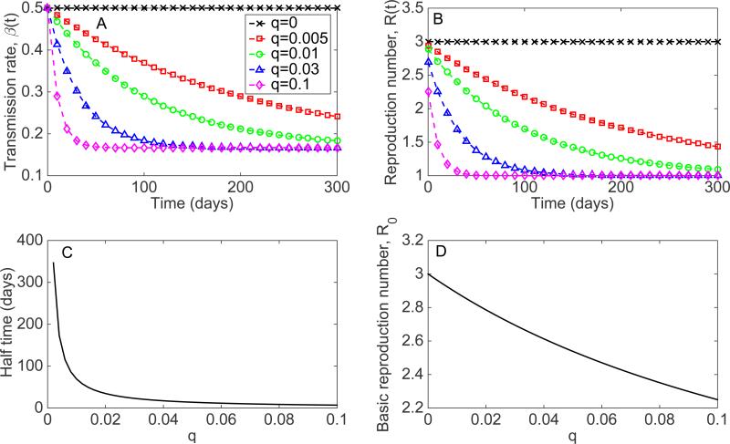
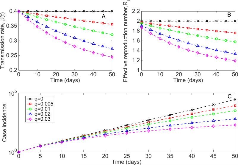
Representative profiles of the time-dependent transmission rate β(t) for different values of the q parameter are shown in Figure 20. The decline rate parameter q can be interpreted through the half time value $\frac{log\left(2\right)}{q}$, the average time elapsed to achieve a transmission rate $\frac{{\beta }_0(1+\varphi )}{2}$ (Figure 20). For a given value of β₀ and γ, the basic reproduction number R₀ is expected to decline from $\frac{{\beta }_0}{\gamma }$ as parameter q increases above 0 (Figure 20). Finally, representative epidemic simulations of early case incidence patterns ranging from sub-exponential to exponential growth dynamics in case incidence derived from this modeling framework are shown in Figure 21.

Figure 20.

A) Representative profiles of the time-dependent transmission rate β(t), B) the effective reproduction number, R_t for different values of the decline rate parameter q and γ = 1/6, β₀ = 0.5 , C) The decline rate parameter q > 0 can be interpreted through the value $\frac{log\left(2\right)}{q}$, which is the mean half time to achieve a transmission rate $\frac{{\beta }_0(1+\varphi )}{2}$, and D) the basic reproduction number as a function of the q parameter. If q = 0, the transmission rate: β(t) = β₀ remains at the baseline value and recovers the standard SEIR transmission dynamics with $R_0=\frac{{\beta }_0}{\gamma }$. Importantly, whenever q > 0 the basic reproduction number, R₀, is no longer simply the product of the initial transmission rate β₀ and the mean infectious period $\frac{1}{\gamma }$ because the transmission rate β(t) declines during the duration of the infectious period. In general, the higher the value of q the faster the decline of the transmission rate towards ϕβ₀ where $\varphi =\frac{\gamma }{{\beta }_0}$ in order to reach an effective reproduction number of 1.0.

Figure 21.

Representative profiles of the transmission rate β(t)(A), the effective reproduction number R_t(B), and corresponding simulations of the early epidemic growth phase (C) derived from the SIR modeling framework described in the text (Equations 5) for different values of the 1 decline rate parameter q, β₀ = 0.4 and $\gamma =\frac{1}{5}$. The epidemic simulations start with one 5 infectious individual. In semi-logarithmic scale, exponential growth is evident if a straight line fits well several consecutive disease generations of the epidemic curve, whereas a strong downward curvature in semi-logarithmic scale is indicative of sub-exponential growth. Our simulations show that case incidence curves display early sub-exponential growth dynamics even for very low values of q.

In the context of HIV/AIDS, prior modeling studies (e.g., [101]) have incorporated a time changing risk in transmission by modeling an exponential decay in the transmission rate in a similar way, except that the rate of decay is a function of the time-dependent prevalence of HIV/AIDS over time and is not bounded below by a reproduction number at 1.0.

3.5 SIR model with inhomogeneous mixing

The SIR model (Equations 5) with a constant transmission rate (β(t) = β₀) is based on mass action kinetics where the incidence rate of the epidemic process is given by ${\beta }_{0}S\left(t\right)\frac{I\left(t\right)}{N}$. This assumes homogenous mixing of the population where every individual in the population has the same probability of contracting the infectious disease. Moreover, the incidence rate increases linearly with the number of infectious individuals, I(t), leading to exponential growth dynamics in the number of infectious individuals at time t, I(t) ≈ I₀e^(β–γ)t. To relax the mass action principle, researchers have incorporated power-law scaling parameters that affect the incidence rate (see e.g., [105-108]). For instance, the incidence rate can take the form: ${\beta }_{0}S\left(t\right)\frac{I^{\alpha }\left(t\right)}{N}$ where 0 < α ≤ 1. Thus, α = 1 models homogeneous mixing while α < 1 captures inhomogeneous mixing that induces slower epidemic growth [108]. The corresponding system of differential equations for this SIR process incorporating inhomogeneous mixing is then given by:

$$\begin{array}{cc}\hfill \frac{dS\left(t\right)}{dt}& =-\beta \left(t\right)S\frac{I^{\alpha }}{N}\hfill \\ \hfill \frac{dI\left(t\right)}{dt}& =\beta \left(t\right)S\frac{I^{\alpha }}{N}-\gamma I\hfill \\ \hfill \frac{dR\left(t\right)}{dt}& =\gamma I\hfill \end{array}$$ (6)

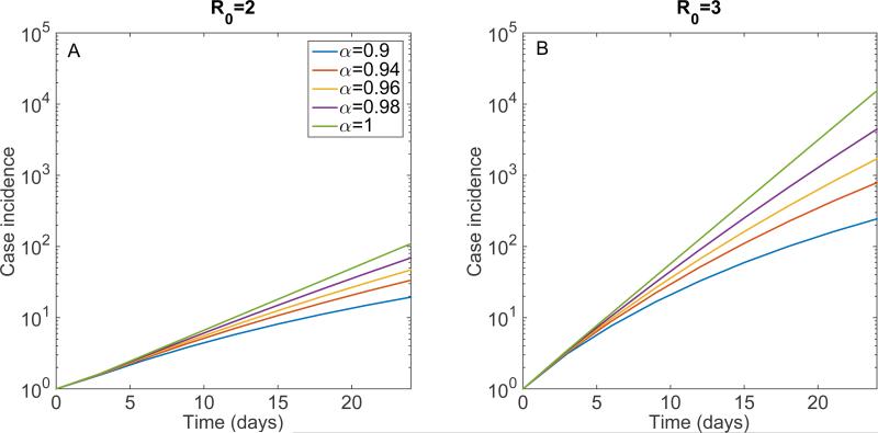
Simulation of this model supports the presence of early sub-exponential growth dynamics even for values of α slightly below the homogenous mixing regime (α = 1) as shown in Figure 22. Indeed, the downward curvature in semi-logarithmic scale of the case incidence curve is indicative of early sub-exponential growth dynamics. It is worth noting that a more elaborate version of this model that relies on the power-law scaling parameter α to capture departures from the homogenous mixing assumption is the well-known TSIR model [24], which has found applications in diverse infectious disease systems (e.g., measles [24,109,110]), rubella [111], and dengue [112]).

Figure 22.

Simulations of the early epidemic growth phase derived from the SIR model 1 described by Equations 6 for different values of the power-law scaling parameter α, $\gamma =\frac{1}{5}$, and 5 (A) β₀ = 0.4, (B) β₀ = 0.6 in a large population size N set at 10⁸. The epidemic simulations start with one infectious individual. In semi-logarithmic scale, exponential growth is evident if a straight line fits well several consecutive disease generations of the epidemic curve, whereas a strong downward curvature in semi-logarithmic scale is indicative of sub-exponential growth. Our simulations show that case incidence curves display early sub-exponential growth dynamics even for values of α slightly below 1.0.

In order to examine the dynamic behavior of the effective reproduction number for the SIR model incorporating inhomogeneous mixing dynamics via the scaling parameter α, we analyzed the temporal progression in the number of cases according to disease generations g [113]. The system of equations is given by:

$$\begin{array}{cc}\hfill I_{g+1}& =S_g(1-e^{-R_0\frac{I_g^{\alpha }}{N}})\hfill \\ \hfill S_{g+1}& =S_g-I_{g+1}\hfill \end{array}$$ (7)

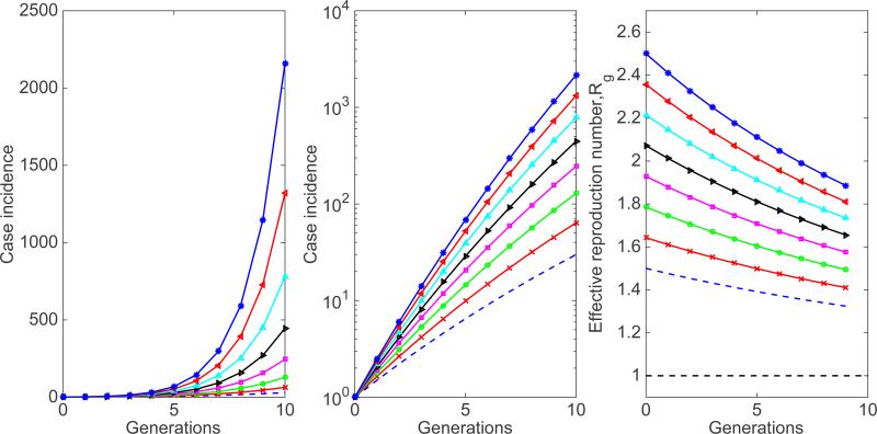
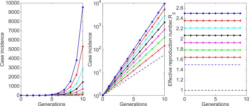
where I_g is the number of new cases at generation g and S_g is the number of remaining susceptibles at generation g. We analyze simulations with I₀ = 1 and S₀ = N where N is a large population size set at 10⁸. Simulations of this model confirm the presence of early sub-exponential growth dynamics for values of α slightly below the homogenous mixing regime at 1.0 as indicated by a downward curvature in case incidence during the fist few generations of disease transmission and a declining effective reproduction number R_g towards 1.0 (Figure 23). By contrast, the effective reproduction number remains invariant during the early epidemic growth phase whenever α = 1 (Figure 24).

Figure 23.

Simulations of the early epidemic growth phase derived from the SIR model based on disease generations described by Equations 7 for different values of the basic reproduction number with a power-law scaling parameter α set at 0.96, just slightly below the homogenous mixing regime (i.e., α = 1), $\gamma =\frac{1}{5}$ and a large population size (N=10⁸). The epidemic simulations start with one infectious individual. Because α < 1, the effective reproduction number according to disease generations, R_g, follows a declining trend towards 1.0. The downward curvature of the case incidence curve in semi-logarithmic scale is also indicative of sub-exponential growth dynamics.

Figure 24.

Simulations of the early epidemic growth phase using the SIR model based on disease generations described by Equations 7 for different values of the basic reproduction number with a power-law scaling parameter α set at 1.0 (i.e., homogenous mixing), $\gamma =\frac{1}{5}$, and a large population size (N=10⁸). The epidemic simulations start with one infectious individual. Because α = 1, the effective reproduction number according to disease generations, R_g, remains invariant during the first few disease generations. As expected, exponential growth during the early growth phase is also evident as a straight line fits well several consecutive disease generations of the epidemic curve.

Discussion

Early epidemic forecasts consisting of the likely short-term trajectory of an unfolding outbreak can help guide the type and intensity of interventions including healthcare infrastructure needs for diagnosis, isolation of infectious individuals, and contact tracing activities [114]. However, our ability to generate disease forecasts using epidemic models during the initial epidemic phase is not only hindered by a lack of reliable epidemiological information and case incidence data, but also by existing gaps in our understanding of the mechanisms involved in the transmission dynamics across different pathogens and social contexts.

A better understanding of the signature features of epidemic outbreaks from real outbreak data and different mathematical modeling approaches could lead to substantial improvements in our ability to forecast epidemics using mathematical modeling. Recent findings have underscored the presence of a variety of early epidemic growth profiles ranging from sub-exponential to exponential growth dynamics across a number of epidemic outbreaks involving different infectious diseases such as pandemic influenza, smallpox, measles, HIV/AIDS and Ebola [5,7]. If early sub-exponential growth dynamics are driven by a spatially constrained contact structure, then transmission models relying on the mass-action mixing assumption tied to early exponential growth dynamics in the absence of interventions or behavior changes would not be supported. This motivates the need to better understand the mechanisms that give rise to slower epidemic growth profiles during the early transmission stages. For instance, the observation that the HIV/AIDS epidemic was spreading in a polynomial fashion rather than exponentially fast can be traced back to the 1980s [9,10]. While these observations were deemed important among experts at the time, developing the classic theory of infectious disease to accommodate the possibility of sub-exponential growth patterns has progressed slowly [5,7,10,24,105,107,108]. More recently, the 2014-15 Ebola epidemic in West Africa has reignited interest in better understanding the processes involved in shaping early sub-exponential growth transmission dynamics of infectious diseases at different spatial scales, their implications in the estimation of key epidemiological quantities, and the development of more accurate models to improve disease forecasting [5]. This review article aims to provide a broad overview of the mechanisms that have been hypothesized to be involved in shaping the early epidemic growth dynamics and to survey relevant results from different mathematical modeling approaches that are available to incorporate such processes in transmission models.

We have briefly reviewed approaches for modeling the spatial or structured spread of infectious diseases using metapopulation models and individual-based models. The analyses of early growth patterns stemming from transmission models can be facilitated by the use of the generalized-growth model which has been recently introduced to characterize profiles of early epidemic growth including sub-exponential and exponential epidemic growth [7]. In addition, both cross-coupled and mobility metapopulation models have proven very useful for generating important insights into how the structuring of human populations and their activities have influenced spatio-temporal patterns of infectious disease spread, and metapopulation or structured models that divide the population into groups can yield early exponential growth of case incidence when the local transmission dynamics are governed by mass-action mixing. Individual-level models provide the modeler with full control over the dynamic interactions of the individuals in the population, however. For instance, individual-based models based on static contact networks provide a way to incorporate explicit measures of clustering, which are known to play a role in slowing down the spread of disease [115]. Indeed, disease spread simulations indicate that a contact network dominated by local (nearest-neighbor) interactions can give rise to early polynomial growth after adding a very small fraction of long-range random links. However, the growth profile quickly approaches an exponential growth regime as the amount of global randomness is slowly increased.

Because disease transmission on “small world” models grounded on static contact networks predict rapid dissemination of disease in the presence of a relatively small fraction of long-range interactions[78], this highlights the potential role of dynamic rather than static contacts in the spread of disease. Indeed, disease-relevant contacts are not static, but dynamic as they change during the course of the day in response to changing perceived disease risk and local customs, and they are also affected by the actual course of individual illness whereby severe cases tend to be confined to specific social settings (e.g., households, hospitals), and hence, are less likely to initiate long-range interactions. The dynamic nature of the contact network implies that the overall population contact network is composed of a group of subnetworks of different sizes that change over time. In this dynamic context, the probability of disease spreading from one individual to another is not a fixed quantity, but depends on the chances that the individuals make a disease-relevant contact during the period of infectiousness of the infector. Therefore, the use of dynamic contact networks for modeling the spread of individual-level disease spread particularly for diseases that spread via close contact (e.g, Ebola, HIV/AIDS) provides the necessary flexibility to incorporate dynamic contact processes (e.g., contact-dependence on behavior, local customs, mobility, and disease status) that may give rise to specific early growth disease transmission patterns in the absence of other disease mitigating factors (e.g., reactive behavior changes, control interventions).

To illustrate the epidemic growth patterns stemming from individual-based models that incorporate more realistic social contact network structures and individual behavior, we analyzed early growth dynamics of disease incidence generated by the detailed Ebola transmission model of Merler et al. [28] and a less complex spatial (household-community) model developed by Kiskowski [26,27]. Interestingly, we found that the model by Merler et al. calibrated to the situation of Liberia yields sub-exponential growth patterns which are well-characterized using the generalized growth model while the spatial model by Kiskowski yields slightly faster growth profiles (although still sub-exponential). These observations suggest that incorporating dynamic contact networks into models of disease spread may be required for modeling more realistic early epidemic growth profiles, while models based on static networks are expected to quickly approach an exponential growth regime in the absence of susceptible depletion or mitigation mechanisms, with the incorporation of a relatively small amount of long-range random interactions even in the presence of substantial levels of clustering [78]. At the same time, our results also underscore substantial uncertainty captured in ensembles of stochastic epidemic realizations.

We have shown that it is feasible to modify the standard SIR compartmental modeling framework to incorporate flexible early epidemic growth profiles ranging from sub-exponential to exponential growth dynamics. This can be achieved, for example, by allowing the effective reproduction number R_t to decline dynamically towards the epidemic threshold at 1.0 to capture early sub-exponential (e.g, polynomial) growth dynamics [101]. This approach is useful to describe a gradual effect of early behavior change that blunts the population transmission (Figure 20). Moreover, we have also shown that the incorporation of a power-law scaling parameter in the incidence rate of the standard SIR modeling framework (${\beta }_{0}S\left(t\right)\frac{I^{\alpha }\left(t\right)}{N}$; see e.g., [105-108]) yields early sub-exponential growth dynamics for values of the scaling parameter α slightly below the homogenous mixing regime at 1.0 as indicated by a downward curvature in simulations of case incidence during the fist few generations of disease transmission and a declining effective reproduction number over R_g towards 1.0 (Figure 23).

The development of infectious disease transmission models guided by qualitative features of observed transmission patterns (e.g, early growth dynamics) is an interesting area ripe for future research that has potential for substantial progress in our ability to generate useful epidemic forecasts for public health decision making. Our review of the literature also indicates an important gap in the classic theory of infectious disease modeling based on compartmental modeling that requires the development of innovative yet tractable mathematical and statistical modeling techniques to incorporate relevant epidemic features such as a flexible spectrum of epidemic growth profiles (e.g., from polynomial to exponential dynamics). At the same time, the increasing availability of computational power provides full flexibility to incorporate dynamic contact processes at the individual level to reproduce particular disease transmission patterns, but their parameterization likely requires datasets whose collection could pose particular challenges. Finally, successful efforts in improving disease transmission modeling towards improved disease forecasting will also have an impact on refining preparedness and contingency intervention plans to confront infectious disease threats.

Figure 7. The 1948 measles epidemic in London.

Representative fits of the generalized-growth model (Equation 1) to an increasing amount of case incidence data during the initial epidemic growth phase (top panels) and the corresponding empirical distribution of the deceleration of growth parameter, p (bottom panel).

Figure 8. The 1905-06 plague epidemic in Bombay, India.

Representative fits of the generalized-growth model (Equation 1) to an increasing amount of case incidence data during the initial epidemic growth phase (top panels) and the corresponding empirical distribution of the deceleration of growth parameter, p (bottom panel).

References

- 1.Anderson RM, May RM. Infectious diseases of humans. Oxford University Press; Oxford: 1991. [Google Scholar]
- 2.Heesterbeek H, Anderson RM, Andreasen V, Bansal S, De Angelis D, et al. Modeling infectious disease dynamics in the complex landscape of global health. Science. 2015;347:aaa4339. doi: 10.1126/science.aaa4339. [DOI] [PMC free article] [PubMed] [Google Scholar]
- 3.Ross R. The Prevention of Malaria. John Murray; London: 1911. [Google Scholar]
- 4.Kermack WO, McKendrick AG. Contributions to the mathematical theory of epidemics: IV. Analysis of experimental epidemics of the virus disease mouse ectromelia. J Hyg (Lond) 1937;37:172–187. doi: 10.1017/s0022172400034902. [DOI] [PMC free article] [PubMed] [Google Scholar]
- 5.Chowell G, Viboud C, Hyman JM, Simonsen L. The Western Africa ebola virus disease epidemic exhibits both global exponential and local polynomial growth rates. PLoS Curr. 2015;7 doi: 10.1371/currents.outbreaks.8b55f4bad99ac5c5db3663e916803261. [DOI] [PMC free article] [PubMed] [Google Scholar]
- 6.Szendroi B, Csányi G. Polynomial epidemics and clustering in contact networks. Proceedings of the Royal Society of London Series B: Biological Sciences. 2004;271:S364–S366. doi: 10.1098/rsbl.2004.0188. [DOI] [PMC free article] [PubMed] [Google Scholar]
- 7.Viboud C, Simonsen L, Chowell G. A generalized-growth model to characterize the early ascending phase of infectious disease outbreaks. Epidemics. 2016;15:27–37. doi: 10.1016/j.epidem.2016.01.002. [DOI] [PMC free article] [PubMed] [Google Scholar]
- 8.Santermans E, Robesyn E, Ganyani T, Sudre B, Faes C, et al. Spatiotemporal Evolution of Ebola Virus Disease at Sub-National Level during the 2014 West Africa Epidemic: Model Scrutiny and Data Meagreness. PLoS One. 2016;11:e0147172. doi: 10.1371/journal.pone.0147172. [DOI] [PMC free article] [PubMed] [Google Scholar]
- 9.May RM, Anderson RM. Transmission dynamics of HIV infection. Nature. 1987;326:137–142. doi: 10.1038/326137a0. [DOI] [PubMed] [Google Scholar]
- 10.Colgate SA, Stanley EA, Hyman JM, Layne SP, Qualls C. Risk behavior-based model of the cubic growth of acquired immunodeficiency syndrome in the United States. Proc Natl Acad Sci U S A. 1989;86:4793–4797. doi: 10.1073/pnas.86.12.4793. [DOI] [PMC free article] [PubMed] [Google Scholar]
- 11.Tolle J. Can Growth Be Faster than Exponential, and Just How Slow Is the Logarithm? The Mathematical Gazette. 2003;87:522–525. [Google Scholar]
- 12.Chowell G, Hincapia-Palacio D, Ospina J, Pell B, Tariq A, et al. Using Phenomenological Models to Characterize Transmissibility and Forecast Patterns and Final Burden of Zika Epidemics. PLOS Currents Outbreaks. 2016 doi: 10.1371/currents.outbreaks.f14b2217c902f453d9320a43a35b9583. [DOI] [PMC free article] [PubMed] [Google Scholar]
- 13.Chowell G, Nishiura H, Bettencourt LM. Comparative estimation of the reproduction number for pandemic influenza from daily case notification data. J R Soc Interface. 2007;4:155–166. doi: 10.1098/rsif.2006.0161. [DOI] [PMC free article] [PubMed] [Google Scholar]
- 14.Wallinga J, Lipsitch M. How generation intervals shape the relationship between growth rates and reproductive numbers. Proc Biol Sci. 2007;274:599–604. doi: 10.1098/rspb.2006.3754. [DOI] [PMC free article] [PubMed] [Google Scholar]
- 15.Meltzer MI, Atkins CY, Santibanez S, Knust B, Petersen BW, et al. Estimating the future number of cases in the ebola epidemic --- liberia and sierra leone, 2014--2015. MMWR Surveill Summ. 2014;63:1–14. [PubMed] [Google Scholar]
- 16.Team WHOER Ebola Virus Disease in West Africa - The First 9 Months of the Epidemic and Forward Projections. N Engl J Med. 2014;371:1481–1495. doi: 10.1056/NEJMoa1411100. [DOI] [PMC free article] [PubMed] [Google Scholar]
- 17.Lewnard JA, Ndeffo Mbah ML, Alfaro-Murillo JA, Altice FL, Bawo L, et al. Dynamics and control of Ebola virus transmission in Montserrado, Liberia: a mathematical modelling analysis. Lancet Infect Dis. 2014;14:1189–1195. doi: 10.1016/S1473-3099(14)70995-8. [DOI] [PMC free article] [PubMed] [Google Scholar]
- 18.Nishiura H, Chowell G. Early transmission dynamics of Ebola virus disease (EVD), West Africa, March to August 2014. Euro Surveill. 2014;19 doi: 10.2807/1560-7917.es2014.19.36.20894. [DOI] [PubMed] [Google Scholar]
- 19.Gomes MF, Piontti AP, Rossi L, Chao D, Longini I, et al. Assessing the International Spreading Risk Associated with the 2014 West African Ebola Outbreak. PLOS Currents Outbreaks. 2014 doi: 10.1371/currents.outbreaks.cd818f63d40e24aef769dda7df9e0da5. [DOI] [PMC free article] [PubMed] [Google Scholar]
- 20.Chowell G, Hengartner NW, Castillo-Chavez C, Fenimore PW, Hyman JM. The basic reproductive number of Ebola and the effects of public health measures: the cases of Congo and Uganda. J Theor Biol. 2004;229:119–126. doi: 10.1016/j.jtbi.2004.03.006. [DOI] [PubMed] [Google Scholar]
- 21.Althaus CL. Estimating the reproduction number of Zaire ebolavirus (EBOV) during the 2014 outbreak in West Africa. PLOS Currents Outbreaks Edition. 2014;1 doi: 10.1371/currents.outbreaks.91afb5e0f279e7f29e7056095255b288. doi: 101371/currentsoutbreaks91afb5e0f279e7f29e7056095255b288. [DOI] [PMC free article] [PubMed] [Google Scholar]
- 22.Drake JM, Kaul RB, Alexander LW, O'Regan SM, Kramer AM, et al. Ebola cases and health system demand in Liberia. PLoS Biol. 2015;13:e1002056. doi: 10.1371/journal.pbio.1002056. [DOI] [PMC free article] [PubMed] [Google Scholar]
- 23.Barbarossa MV, Denes A, Kiss G, Nakata Y, Rost G, et al. Transmission Dynamics and Final Epidemic Size of Ebola Virus Disease Outbreaks with Varying Interventions. PLoS One. 2015;10:e0131398. doi: 10.1371/journal.pone.0131398. [DOI] [PMC free article] [PubMed] [Google Scholar]
- 24.Finkenstädt BF, Grenfell BT. Time series modelling of childhood diseases: a dynamical systems approach. Appl Stat. 2000;49:187–205. [Google Scholar]
- 25.Grenfell BT, Bjornstad ON, Kappey J. Travelling waves and spatial hierarchies in measles epidemics. Nature. 2001;414:716–723. doi: 10.1038/414716a. [DOI] [PubMed] [Google Scholar]
- 26.Kiskowski M, Chowell G. Modeling household and community transmission of Ebola virus disease: epidemic growth, spatial dynamics and insights for epidemic control. Virulence. 2015;7:63–73. doi: 10.1080/21505594.2015.1076613. [DOI] [PMC free article] [PubMed] [Google Scholar]
- 27.Kiskowski M. Three-Scale Network Model for the Early Growth Dynamics of 2014. West Africa Ebola Epidemic. PLOS Currents Outbreaks. 2014 doi: 10.1371/currents.outbreaks.c6efe8274dc55274f05cbcb62bbe6070. doi: 101371/currents.outbreaks.b4690859d91684da963dc40e00f3da81. [DOI] [PMC free article] [PubMed] [Google Scholar]
- 28.Merler S, Ajelli M, Fumanelli L, Gomes MF, Piontti AP, et al. Spatiotemporal spread of the 2014 outbreak of Ebola virus disease in Liberia and the effectiveness of non-pharmaceutical interventions: a computational modelling analysis. Lancet Infect Dis. 2015;15:204–211. doi: 10.1016/S1473-3099(14)71074-6. [DOI] [PMC free article] [PubMed] [Google Scholar]
- 29.Keeling MJ, Woolhouse ME, May RM, Davies G, Grenfell BT. Modelling vaccination strategies against foot-and-mouth disease. Nature. 2003;421:136–142. doi: 10.1038/nature01343. [DOI] [PubMed] [Google Scholar]
- 30.Ferguson NM, Donnelly CA, Anderson RM. The foot-and-mouth epidemic in Great Britain: pattern of spread and impact of interventions. Science. 2001;292:1155–1160. doi: 10.1126/science.1061020. [DOI] [PubMed] [Google Scholar]
- 31.Chowell G, Rivas AL, Hengartner NW, Hyman JM, Castillo-Chavez C. The role of spatial mixing in the spread of foot-and-mouth disease. Prev Vet Med. 2006;73:297–314. doi: 10.1016/j.prevetmed.2005.10.002. [DOI] [PubMed] [Google Scholar]
- 32.Riley S, Ferguson NM. Smallpox transmission and control: spatial dynamics in Great Britain. Proc Natl Acad Sci U S A. 2006;103:12637–12642. doi: 10.1073/pnas.0510873103. [DOI] [PMC free article] [PubMed] [Google Scholar]
- 33.Halloran ME, Longini IM, Jr., Nizam A, Yang Y. Containing bioterrorist smallpox. Science. 2002;298:1428–1432. doi: 10.1126/science.1074674. [DOI] [PubMed] [Google Scholar]
- 34.Eubank S, Guclu H, Kumar VS, Marathe MV, Srinivasan A, et al. Modelling disease outbreaks in realistic urban social networks. Nature. 2004;429:180–184. doi: 10.1038/nature02541. [DOI] [PubMed] [Google Scholar]
- 35.Chowell G, Viboud C, Simonsen L, Moghadas SM. Characterizing the reproduction number of epidemics with early sub-exponential growth dynamics. 2016 doi: 10.1098/rsif.2016.0659. http://arxivorg/abs/160301216. [DOI] [PMC free article] [PubMed]
- 36.Davis S, Trapman P, Leirs H, Begon M, Heesterbeek JA. The abundance threshold for plague as a critical percolation phenomenon. Nature. 2008;454:634–637. doi: 10.1038/nature07053. [DOI] [PubMed] [Google Scholar]
- 37.Salkeld DJ, Salathe M, Stapp P, Jones JH. Plague outbreaks in prairie dog populations explained by percolation thresholds of alternate host abundance. Proc Natl Acad Sci U S A. 2010;107:14247–14250. doi: 10.1073/pnas.1002826107. [DOI] [PMC free article] [PubMed] [Google Scholar]
- 38.Cross PC, Johnson PL, Lloyd-Smith JO, Getz WM. Utility of R0 as a predictor of disease invasion in structured populations. J R Soc Interface. 2007;4:315–324. doi: 10.1098/rsif.2006.0185. [DOI] [PMC free article] [PubMed] [Google Scholar]
- 39.Bailey NTJ. The mathematical theory of infectious disease and its applications. Hafner; New York: 1975. [Google Scholar]
- 40.Brockman D, Helbing D. The hidden geometry of complex, network-driven contagion phenomena. Science. 2013:1337–1342. doi: 10.1126/science.1245200. [DOI] [PubMed] [Google Scholar]
- 41.Riley S. Large-scale spatial-transmission models of infectious disease. Science. 2007;316:1298–1301. doi: 10.1126/science.1134695. [DOI] [PubMed] [Google Scholar]
- 42.Wilson EB, Worcester J. The spread of an epidemic. Proc Natl Acad Sci USA. 1945;31:327–333. doi: 10.1073/pnas.31.10.327. [DOI] [PMC free article] [PubMed] [Google Scholar]
- 43.Rushton SP, Mautner A. The deterministic model of a simple epidemic for more than one community. Biometrika. 1955;42 [Google Scholar]
- 44.Sattenspiel L. The geographic spread of infectious diseases: models and applications. Princeton University Press; 2009. [Google Scholar]
- 45.Keeling MJ, Rohani P. Modeling infectious diseases in humans and animals. Princeton University Press; 2008. [Google Scholar]
- 46.Vincenot CE, Moriya K. Impact of the topology of metapopulations on the resurgence of epidemics rendered by a new multiscale hybrid modeling approach. Ecol Inform. 2011;6 doi: 10.1016/j.ecoinf.2011.04.002. [DOI] [PMC free article] [PubMed] [Google Scholar]
- 47.Apolloni A, Poletto C, Ramasco JJ, Jensen P, Colizza V. Metapopulation epidemic models with heterogeneous mixing and travel behaviour. Theor Biol Med Model. 2014;11:3. doi: 10.1186/1742-4682-11-3. [DOI] [PMC free article] [PubMed] [Google Scholar]
- 48.Belik V, Geisel T, Brockmann D. Natural human mobility patterns and spatial spread of infectious diseases. Phys Rev X. 2011;1 [Google Scholar]
- 49.Xiao Y, Zhou Y, Tang S. Modelling disease spread in dispersal networks at two levels. Math Med Biol. 2011;28:227–244. doi: 10.1093/imammb/dqq007. [DOI] [PubMed] [Google Scholar]
- 50.Kenah E, Chao DL, Matrajt L, Halloran ME, Longini IM., Jr The global transmission and control of influenza. PLoS One. 2011;6:e19515. doi: 10.1371/journal.pone.0019515. [DOI] [PMC free article] [PubMed] [Google Scholar]
- 51.Marguta R, Parisi A. Impact of human mobility on the periodicities and mechanisms underlying measles dynamics. J R Soc Interface. 2015;12:20141317. doi: 10.1098/rsif.2014.1317. [DOI] [PMC free article] [PubMed] [Google Scholar]
- 52.Appoloni A, Poletto C, Colizza V. Age-specific contacts and travel patterns in the spatial spread of 2009 H1N1 influenza pandemic. BMC Infect Dis. 2013;13:176. doi: 10.1186/1471-2334-13-176. [DOI] [PMC free article] [PubMed] [Google Scholar]
- 53.Tizzoni M, Bajardi P, Poletto C, Ramasco JJ, Balcan D, et al. Real-time numerical forecast of global epidemic spreading: case study of 2009 A/H1N1pdm. BMC Med. 2012;10:165. doi: 10.1186/1741-7015-10-165. [DOI] [PMC free article] [PubMed] [Google Scholar]
- 54.Arino J, Jordan R, van den Driessche P. Quarantine in a multi-species epidemic model with spatial dynamics. Math Biosci. 2007;206:46–60. doi: 10.1016/j.mbs.2005.09.002. [DOI] [PubMed] [Google Scholar]
- 55.Murray GD, Cliff AD. A stochastic model for measles epidemics in a multi-region setting. Trans Inst Br Geogr. 1977;2:158–174. [Google Scholar]
- 56.Sattenspiel L, Dietz K. A structured epidemic model incorporating geographic mobility among regions. Math Biosci. 1995;128:71–91. doi: 10.1016/0025-5564(94)00068-b. [DOI] [PubMed] [Google Scholar]
- 57.Xia YC, Bjørnstad ON, Grenfell BT. Measles metapopulation dynamics: a gravity model for epidemiological coupling and dynamics. Am Nat. 2004;164:267–281. doi: 10.1086/422341. [DOI] [PubMed] [Google Scholar]
- 58.Weinberger DM, Krause TG, Molbak K, Cliff A, Briem H, et al. Influenza epidemics in Iceland over 9 decades: changes in timing and synchrony with the United States and Europe. Am J Epidemiol. 2012;176:649–655. doi: 10.1093/aje/kws140. [DOI] [PMC free article] [PubMed] [Google Scholar]
- 59.Viboud C, Bjornstad ON, Smith DL, Simonsen L, Miller MA, et al. Synchrony, waves, and spatial hierarchies in the spread of influenza. Science. 2006;312:447–451. doi: 10.1126/science.1125237. [DOI] [PubMed] [Google Scholar]
- 60.Simini P, González MC, Maritan A, Barabási A-L. A universal model for mobility and migration patterns. Nature. 2012;484:96–100. doi: 10.1038/nature10856. [DOI] [PubMed] [Google Scholar]
- 61.Tizzoni M, Bajardi P, Decuyper A, King G, Schneider CM, et al. On the use of human mobility proxies for modeling epidemics. PLoS Comput Biol. 2014;10:e1003716. doi: 10.1371/journal.pcbi.1003716. [DOI] [PMC free article] [PubMed] [Google Scholar]
- 62.Ajelli M, Gonçalves B, Balcan D, Colizza V, Hu H, et al. Comparing large-scale computational approaches to epidemic modeling: agent-based versus structured metapopulation models. BMC Infect Dis. 2010;10:190. doi: 10.1186/1471-2334-10-190. [DOI] [PMC free article] [PubMed] [Google Scholar]
- 63.Ball F, Britton T, House T, Isham V, Mollison D, et al. Seven challenges for metapopulation models of epidemics, including households models. Epidemics. 2015;10:63–67. doi: 10.1016/j.epidem.2014.08.001. [DOI] [PubMed] [Google Scholar]
- 64.Tamerius J, Viboud C, Shaman J, Chowell G. Impact of School Cycles and Environmental Forcing on the Timing of Pandemic Influenza Activity in Mexican States, May-December 2009. PLoS Comput Biol. 2015;11:e1004337. doi: 10.1371/journal.pcbi.1004337. [DOI] [PMC free article] [PubMed] [Google Scholar]
- 65.Burger R, Chowell G, Mulet P, Villada LM. Modelling the spatial-temporal progression of the 2009 A/H1N1 influenza pandemic in Chile. Math Biosci Eng. 2016;13:43–65. doi: 10.3934/mbe.2016.13.43. [DOI] [PubMed] [Google Scholar]
- 66.Balcan D, Hu H, Goncalves B, Bajardi P, Poletto C, et al. Seasonal transmission potential and activity peaks of the new influenza A(H1N1): a Monte Carlo likelihood analysis based on human mobility. BMC Med. 2009;7:45. doi: 10.1186/1741-7015-7-45. [DOI] [PMC free article] [PubMed] [Google Scholar]
- 67.Van den Broeck W, Gioannini C, Goncalves B, Quaggiotto M, Colizza V, et al. The GLEaMviz computational tool, a publicly available software to explore realistic epidemic spreading scenarios at the global scale. BMC Infect Dis. 2011;11:37. doi: 10.1186/1471-2334-11-37. [DOI] [PMC free article] [PubMed] [Google Scholar]
- 68.The Global Epidemic and Mobility Model. [01 March 2016];GLEAMviz. Available from: http://www.gleamviz.org/simulator/client/
- 69.Bansal S, Grenfell BT, Meyers LA. When individual behaviour matters: homogeneous and network models in epidemiology. Journal of the Royal Society Interface. 2007;4:879–891. doi: 10.1098/rsif.2007.1100. [DOI] [PMC free article] [PubMed] [Google Scholar]
- 70.Danon L, Ford AP, House T, Jewell CP, Keeling MJ, et al. Networks and the epidemiology of infectious disease. Interdiscip Perspect Infect Dis. 2011;2011:284909. doi: 10.1155/2011/284909. [DOI] [PMC free article] [PubMed] [Google Scholar]
- 71.Keeling MJ, Eames KT. Networks and epidemic models. J R Soc Interface. 2005;2:295–307. doi: 10.1098/rsif.2005.0051. [DOI] [PMC free article] [PubMed] [Google Scholar]
- 72.Wylie JL, Jolly A. Patterns of chlamydia and gonorrhea infection in sexual networks in Manitoba, Canada. Sex Transm Dis. 2001;28:14–24. doi: 10.1097/00007435-200101000-00005. [DOI] [PubMed] [Google Scholar]
- 73.Eames KT, Keeling MJ. Monogamous networks and the spread of sexually transmitted diseases. Math Biosci. 2004;189:115–130. doi: 10.1016/j.mbs.2004.02.003. [DOI] [PubMed] [Google Scholar]
- 74.Christley RM, Pinchbeck GL, Bowers RG, Clancy D, French NP, et al. Infection in social networks: using network analysis to identify high-risk individuals. Am J Epidemiol. 2005;162:1024–1031. doi: 10.1093/aje/kwi308. [DOI] [PubMed] [Google Scholar]
- 75.Meyers LA, Pourbohloul B, Newman ME, Skowronski DM, Brunham RC. Network theory and SARS: predicting outbreak diversity. J Theor Biol. 2005;232:71–81. doi: 10.1016/j.jtbi.2004.07.026. [DOI] [PMC free article] [PubMed] [Google Scholar]
- 76.Drewe JA. Who infects whom? Social networks and tuberculosis transmission in wild meerkats. Proc Biol Sci. 2010;277:633–642. doi: 10.1098/rspb.2009.1775. [DOI] [PMC free article] [PubMed] [Google Scholar]
- 77.Bansal S, Pourbohloul B, Hupert N, Grenfell B, Meyers LA. The shifting demographic landscape of pandemic influenza. PLoS One. 2010;5:e9360. doi: 10.1371/journal.pone.0009360. [DOI] [PMC free article] [PubMed] [Google Scholar]
- 78.Watts DJ, Strogatz SH. Collective dynamics of 'small-world' networks. Nature. 1998;393:440–442. doi: 10.1038/30918. [DOI] [PubMed] [Google Scholar]
- 79.Pastor-Satorras R, Vespignani A. Epidemic spreading in scale-free networks. Phys Rev Lett. 2001;86:3200–3203. doi: 10.1103/PhysRevLett.86.3200. [DOI] [PubMed] [Google Scholar]
- 80.Molloy M, Reed B. A Critical-Point for Random Graphs with a Given Degree Sequence. Random Structures & Algorithms. 1995;6:161–179. [Google Scholar]
- 81.Volz E. SIR dynamics in random networks with heterogeneous connectivity. Journal of Mathematical Biology. 2008;56:293–310. doi: 10.1007/s00285-007-0116-4. [DOI] [PMC free article] [PubMed] [Google Scholar]
- 82.Miller JC, Volz EM. Incorporating disease and population structure into models o f SIR disease in contact networks. PLoS One. 2013;8:e69162. doi: 10.1371/journal.pone.0069162. [DOI] [PMC free article] [PubMed] [Google Scholar]
- 83.Newman ME. Spread of epidemic disease on networks. Phys Rev E Stat Nonlin Soft Matter Phys. 2002;66:016128. doi: 10.1103/PhysRevE.66.016128. [DOI] [PubMed] [Google Scholar]
- 84.Smilkov D, Hidalgo CA, Kocarev L. Beyond network structure: How heterogeneous susceptibility modulates the spread of epidemics. Scientific Reports. 2014;4 doi: 10.1038/srep04795. [DOI] [PMC free article] [PubMed] [Google Scholar]
- 85.Wasserman S. Social network analysis: Methods and applications. Cambridge university press; 1994. [Google Scholar]
- 86.Lloyd ALVS, Cintrón-Arias A. Infection dynamics on small-world networks. Contemp Math. 2006;410:209. [Google Scholar]
- 87.Keeling MJ. The effects of local spatial structure on epidemiological invasions. Proc Biol Sci. 1999;266:859–867. doi: 10.1098/rspb.1999.0716. [DOI] [PMC free article] [PubMed] [Google Scholar]
- 88.Eames KT, Keeling MJ. Modeling dynamic and network heterogeneities in the spread of sexually transmitted diseases. Proc Natl Acad Sci U S A. 2002;99:13330–13335. doi: 10.1073/pnas.202244299. [DOI] [PMC free article] [PubMed] [Google Scholar]
- 89.Keeling M. The implications of network structure for epidemic dynamics. Theor Popul Biol. 2005;67:1–8. doi: 10.1016/j.tpb.2004.08.002. [DOI] [PubMed] [Google Scholar]
- 90.Eames KT. Modelling disease spread through random and regular contacts in clustered populations. Theor Popul Biol. 2008;73:104–111. doi: 10.1016/j.tpb.2007.09.007. [DOI] [PubMed] [Google Scholar]
- 91.Dangerfield CE, Ross JV, Keeling MJ. Integrating stochasticity and network structure into an epidemic model. J R Soc Interface. 2009;6:761–774. doi: 10.1098/rsif.2008.0410. [DOI] [PMC free article] [PubMed] [Google Scholar]
- 92.Bansal S, Read J, Pourbohloul B, Meyers LA. The dynamic nature of contact networks in infectious disease epidemiology. J Biol Dyn. 2010;4:478–489. doi: 10.1080/17513758.2010.503376. [DOI] [PubMed] [Google Scholar]
- 93.Volz E, Meyers LA. Epidemic thresholds in dynamic contact networks. J R Soc Interface. 2009;6:233–241. doi: 10.1098/rsif.2008.0218. [DOI] [PMC free article] [PubMed] [Google Scholar]
- 94.Smieszek T, Fiebig L, Scholz RW. Models of epidemics: when contact repetition and clustering should be included. Theor Biol Med Model. 2009;6:11. doi: 10.1186/1742-4682-6-11. [DOI] [PMC free article] [PubMed] [Google Scholar]
- 95.Read JM, Eames KT, Edmunds WJ. Dynamic social networks and the implications for the spread of infectious disease. J R Soc Interface. 2008;5:1001–1007. doi: 10.1098/rsif.2008.0013. [DOI] [PMC free article] [PubMed] [Google Scholar]
- 96.Kretzschmar M, Morris M. Measures of concurrency in networks and the spread of infectious disease. Math Biosci. 1996;133:165–195. doi: 10.1016/0025-5564(95)00093-3. [DOI] [PubMed] [Google Scholar]
- 97.Britton TJD, Saldana J. A network epidemic model with preventive rewiring: comparative analysis of the initial phase. 2015 doi: 10.1007/s11538-016-0227-4. Available: http://arxivorg/abs/151200344. [DOI] [PubMed]
- 98.Fenichel EP, Castillo-Chavez C, Ceddia MG, Chowell G, Parra PA, et al. Adaptive human behavior in epidemiological models. Proc Natl Acad Sci U S A. 2011;108:6306–6311. doi: 10.1073/pnas.1011250108. [DOI] [PMC free article] [PubMed] [Google Scholar]
- 99.Funk S, Salathe M, Jansen VA. Modelling the influence of human behaviour on the spread of infectious diseases: a review. J R Soc Interface. 2010;7:1247–1256. doi: 10.1098/rsif.2010.0142. [DOI] [PMC free article] [PubMed] [Google Scholar]
- 100.Funk S, Bansal S, Bauch CT, Eames KT, Edmunds WJ, et al. Nine challenges in incorporating the dynamics of behaviour in infectious diseases models. Epidemics. 2015;10:21–25. doi: 10.1016/j.epidem.2014.09.005. [DOI] [PubMed] [Google Scholar]
- 101.Granich RM, Gilks CF, Dye C, De Cock KM, Williams BG. Universal voluntary HIV testing with immediate antiretroviral therapy as a strategy for elimination of HIV transmission: a mathematical model. Lancet. 2009;373:48–57. doi: 10.1016/S0140-6736(08)61697-9. [DOI] [PubMed] [Google Scholar]
- 102.Kermack WO, McKendrick AG. Contributions to the mathematical theory of epidemics--I. 1927. Bull Math Biol. 1991;53:33–55. doi: 10.1007/BF02464423. [DOI] [PubMed] [Google Scholar]
- 103.Bacaer N, Ait Dads el H. Genealogy with seasonality, the basic reproduction number, and the influenza pandemic. J Math Biol. 2011;62:741–762. doi: 10.1007/s00285-010-0354-8. [DOI] [PubMed] [Google Scholar]
- 104.Bacaer N. The model of Kermack and McKendrick for the plague epidemic in Bombay and the type reproduction number with seasonality. J Math Biol. 2012;64:403–422. doi: 10.1007/s00285-011-0417-5. [DOI] [PubMed] [Google Scholar]
- 105.Liu WM, Hethcote HW, Levin SA. Dynamical behavior of epidemiological models with nonlinear incidence rates. J Math Biol. 1987;25:359–380. doi: 10.1007/BF00277162. [DOI] [PubMed] [Google Scholar]
- 106.Liu WM, Levin SA, Iwasa Y. Influence of nonlinear incidence rates upon the behavior of SIRS epidemiological models. J Math Biol. 1986;23:187–204. doi: 10.1007/BF00276956. [DOI] [PubMed] [Google Scholar]
- 107.Hochberg ME. Non-linear transmission rates and the dynamics of infectious disease. J Theor Biol. 1991;153:301–321. doi: 10.1016/s0022-5193(05)80572-7. [DOI] [PubMed] [Google Scholar]
- 108.Severo N. Generalizations of some stochastic epidemic models. Mathematical Biosciences. 1969;4:395–402. [Google Scholar]
- 109.Grenfell BT, Bjornstad ON, Finkenstadt BF. Dynamics of measles epidemics: Scaling noise, determinism, and predictability with the TSIR model. Ecological Monographs. 2002;72:185–202. [Google Scholar]
- 110.Ferrari MJ, Grais RF, Bharti N, Conlan AJ, Bjornstad ON, et al. The dynamics of measles in sub-Saharan Africa. Nature. 2008;451:679–684. doi: 10.1038/nature06509. [DOI] [PubMed] [Google Scholar]
- 111.Metcalf CJ, Munayco CV, Chowell G, Grenfell BT, Bjornstad ON. Rubella metapopulation dynamics and importance of spatial coupling to the risk of congenital rubella syndrome in Peru. J R Soc Interface. 8:369–376. doi: 10.1098/rsif.2010.0320. [DOI] [PMC free article] [PubMed] [Google Scholar]
- 112.Kraemer MU, Perkins TA, Cummings DA, Zakar R, Hay SI, et al. Big city, small world: density, contact rates, and transmission of dengue across Pakistan. J R Soc Interface. 2015;12:20150468. doi: 10.1098/rsif.2015.0468. [DOI] [PMC free article] [PubMed] [Google Scholar]
- 113.Becker NG. Modeling to inform infectious disease control. Chapman and Hall/CRC; 2015. [Google Scholar]
- 114.Chretien JP, George D, Shaman J, Chitale RA, McKenzie FE. Influenza forecasting in human populations: a scoping review. PLoS One. 2014;9:e94130. doi: 10.1371/journal.pone.0094130. [DOI] [PMC free article] [PubMed] [Google Scholar]
- 115.Miller JC. Spread of infectious disease through clustered populations. J R Soc Interface. 2009;6:1121–1134. doi: 10.1098/rsif.2008.0524. [DOI] [PMC free article] [PubMed] [Google Scholar]