Abstract
Disease alters tissue microstructure, which in turn affects the macroscopic mechanical properties of tissue. In elasticity imaging, the macroscopic response is measured and is used to infer the spatial distribution of the elastic constitutive parameters. When an empirical constitutive model is used these parameters cannot be linked to the microstructure. However, when the constitutive model is derived from a microstructural representation of the material, it allows for the possibility of inferring the local averages of the spatial distribution of the microstructural parameters. This idea forms the basis of this study. In particular, we first derive a constitutive model by homogenizing the mechanical response of a network of elastic, tortuous fibers. Thereafter, we use this model in an inverse problem to determine the spatial distribution of the microstructural parameters. We solve the inverse problem as a constrained minimization problem, and develop efficient methods for solving it. We apply these methods to displacement fields obtained by deforming gelatin-agar co-gels, and determine the spatial distribution of agar concentration and fiber tortuosity, thereby demonstrating that it is possible to image local averages of microstructural parameters from macroscopic measurements of deformation.
Keywords: Microstructure Imaging, Elasticity Imaging, Homogenization, Gelatin-Agar Co-Gels
1 Introduction
Several diseases lead to changes in tissue microstructure. For example, the progression of an invasive phenotype in breast cancer is accompanied by an increase in the concentration of collagen [Kass et al., 2007]; and in later stages, by a significant reduction in the tortuosity of the collagen fibers [Provenzano et al., 2006]. Similarly, cirrhosis in the liver is accompanied by an increase in the concentration of collagen [Wells, 2013]. Changes in microstructural organization of the type described above, in turn lead to changes in the macroscopic mechanical properties of tissue. For instance, an increase in collagen concentration within certain regions of the breast and the liver, typically leads to a higher elastic modulus in these regions. The reduction in the tortuosity of collagen fibers in malignant breast tumors leads to an enhanced nonlinear elastic response of the tissue within these tumors [Goenezen et al., 2012].
These macroscopic changes in the mechanical properties of tissue can be measured using a group of techniques that are collectively referred to as elasticity imaging [Ophir et al., 1991, Parker et al., 2005, Barbone and Oberai, 2010]. In elasticity imaging, images of the mechanical properties of tissue are generated by making use of conventional imaging techniques such as ultrasound, magnetic resonance imaging or optical coherence tomography. The basic process involves imaging the tissue as it deforms (in response to an internal or an external excitation) using a conventional imaging technique, and then using the sequence of images thus obtained to determine the displacement field within the tissue. Once this field is known, it may be used in conjunction with the equations of balance of linear momentum and an appropriate mechanical model (constitutive law) in order to determine the spatial distribution of the mechanical properties of tissue. Elasticity imaging has now been used to diagnose different types of diseases. In particular, high linear and nonlinear elastic parameter values in breast tumors have been used to distinguish malignant lesions from benign lesions [Berg et al., 2012, Goenezen et al., 2012] and a high value of the the linear elastic modulus of liver has been used to diagnose liver fibrosis [Talwalkar et al., 2007, Huwart et al., 2008].
While the applications of elasticity imaging described above are exciting and carry a lot of promise, they have thus far used phenomenologically derived constitutive models. In most applications, a linear elastic and isotropic constitutive model has been used, and in a few cases with finite deformation an exponential-type stress strain law has been used. A natural extension of these ideas is to consider constitutive relations that are derived from a microstructural model for the tissue [Lanir, 1979, Lanir, 1983, Cacho et al., 2007, Billiar and Sacks, 2000a, Billiar and Sacks, 2000b]. With these models elasticity imaging could be used to determine the spatial distribution of parameters that are directly linked to the microstructure. As a result it will offer a more direct evaluation of the health of the tissue. It might also be used to understand the microstructural reorganization that takes place during disease progression. This extension of elasticity imaging to a technique that can be used to image microstructural parameters is the main topic of this paper.
As a model for the microstructure, we consider a network of fibers where each fiber is parameterized by its linear stiffness and its tortuosity. Similar models have been utilized by several authors in the past [Lanir, 1979, Lanir, 1983, Cacho et al., 2007, Billiar and Sacks, 2000a, Billiar and Sacks, 2000b]. Thereafter we use a simple homogenization approach to determine the macroscopic mechanical behavior, that is the constitutive model, of a material that is comprised of a network of these fibers. In determining this response we do not solve a microscopic problem; rather we assume that the microscopic deformation is equal to the applied macroscopic stretch, which is the so-called affine assumption. We account for the violation of this assumption by introducing a correction factor (determined from [Shahsavari and Picu, 2012]) in the macroscopic response. Once the macroscopic constitutive model is developed, we use it in the formulation of the inverse problem of interest, which reads as follows: Given the displacement field in the specimen, determine the spatial distribution of the material parameters, and hence the microstructural mechanical parameters, within the specimen. We apply this approach to specimens made from gelatin-agarose co-gels, and determine the spatial distribution of two microstructural parameters: agar concentration, and effective fiber tortuosity from displacement estimates. For both properties we compare our predictions with independent benchmarks and note that we are able to estimate these parameters quite accurately.
The format of the remainder of this paper is as follows: In Section 2 we derive our microstructure-based constitutive model. In Section 3, we define the strong and the weak form of the forward problem corresponding to this model. In Section 4, we define the corresponding inverse problem as a constrained minimization problem, and describe an efficient method for solving this problem. In Section 5, we consider a synthetic (computer-generated data) inverse problem to test our numerical method. In Section 6, we apply our approach to determine the spatial distribution of microstructural parameters of gelatin-agar co-gels. We end with conclusions in Section 7.
2 Microstructure-based Constitutive Model
2.1 Model for an individual wavy fiber
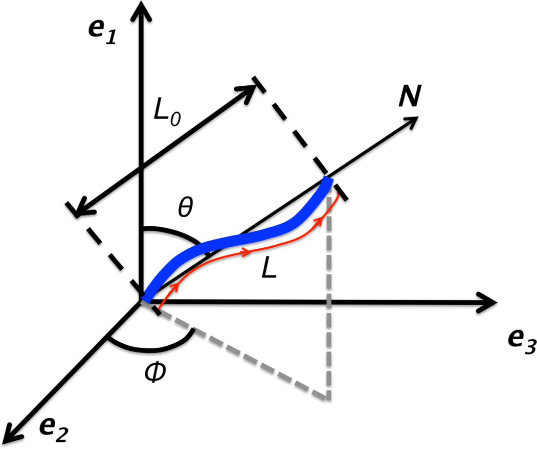
In order to model the mechanics of a tortuous fiber, it is assumed that it is wavy in its unloaded state, and is characterized by its stiffness κ, and the nonlinear parameter γ, which is a measure of fiber tortuosity τ0. The tortuosity is defined as the ratio of path-length, L, to the end-to-end length, L0, as shown in Figure 1. The force-stretch relation for a single fiber with orientation θ = [θ, ϕ] is given by
| (1) |
where, λθ is the stretch of the fiber. We note that the exponential form of this expression is motivated by previous work [Billiar and Sacks, 2000a, Billiar and Sacks, 2000b]. However, within the exponential we use the stretch, and not its square. This allows us to obtain a simple relation between the nonlinear parameter and the tortuosity of the fiber. The role of κ and γ in determining the mechanical response of the fiber is described in Appendix A.
Fig. 1.
Schematic diagram of a wavy fiber with orientation θ = [θ, ϕ]
Let us consider a wavy fiber with tortuosity τ0 that is subject to a force. The stiffness of the fiber at different values of stretch is quantified by the slope of the force-stretch curve. We expect this stiffness to vary as a function of the stretch. In particular, when the value of the applied stretch approaches the value of the tortuosity we expect the stiffness of the fiber to increase substantially. We may use this behavior as a means to infer the tortuosity of fiber. In particular, we say the tortuosity of the fiber may be estimated by the value of stretch at which the stiffness of the fiber is two times its stiffness at zero strain. For the specific force-stretch relation that we have assumed (1), this yields,
| (2) |
From equation (2), we observe that tortuosity τ0 is approximately equal to one plus the inverse of nonlinear parameter γ. Thus a fiber with a large value of tortuosity will have a smaller value for the nonlinear parameter. We note that the choice of the ratio (selected to be 2 in the relation above) is arbitrary. In effect, we could have chosen any number C > 1. In that case the analysis above would have yielded
| (3) |
Even in this case we note that γ is an inverse measure of the tortuosity of the fiber.
In the next subsection, we will evaluate the strain energy of a homogenized material as the sum of the strain energy of individual fibers. For this we first estimate the strain energy associated with a single fiber,
| (4) |
where
| (5) |
2.2 Modeling fibrous materials
In this section we derive an expression for the total strain energy density function for materials that are comprised of a collection of fibers of the type described in the previous section. At every point in the material we assume the existence of density function n̂(θ), such that the product n̂(θ)dθ represents the number of fibers per unit volume with orientation in the interval (θ, θ + dθ) × (ϕ, ϕ + dϕ).
The total strain energy density function for the composite material with the fibers is obtained by integrating the strain energy density for fibers over all possible orientations. This yields,
| (6) |
For an isotropic distribution of fibers the density function n̂(θ) is independent of θ, and is given by , where n is the number density of fibers per unit volume. In this case, the total strain energy density function reduces to [Gasser et al., 2006, Miehe et al., 2002, Garikipati et al., 2008, Alastrué et al., 2009]
| (7) |
The λθ appears in (7) is the stretch for a fiber with a given orientation θ. It is different for each fiber, and in general its value must be evaluated by applying a macroscopic stretch to a representative volume element, and then evaluating the individual stretch of each fiber. An approximation to this value is obtained by making the so-called affine assumption [Lanir, 1979]. Here the stretch for each fiber is approximated as the macroscopic stretch projected along the orientation of the fiber, that is
| (8) |
where N(θ, ϕ) = [cos θ, sin θ cos ϕ, sin θ sin ϕ] is the unit vector along the fiber orientation, C is the right Cauchy-Green strain tensor associated with the macroscopic stretch.
Several studies have assumed affine deformation for collagen fibers [Billiar and Sacks, 2000a, Zulliger et al., 2004]. It is a convenient assumption since it circumvents solving a microscopic problem in order to determine the response of fibers oriented along arbitrary directions. However, recent studies have suggested that the deformation of a typical network might be actually be non-affine [Head et al., 2003a, Head et al., 2003b, Wilhelm and Frey, 2003]. For instance, in an experimental investigation of porcine aortic valve leaflets and bovine pericardium, Billiar [Billiar and Sacks, 1997] reported that fiber networks undergo non-affine deformation. In [Liu et al., 2007] the authors found that cross-linked actin networks are dominated by non-affine deformation at shear strains between 10 % and 30 %. In [Shahsavari and Picu, 2012] it was observed that non-affine deformations are promoted in networks with lower concentration of fibers, and by fibers for which bending energy is more significant than axial strain energy.
When the deformation of the network is assumed to be affine, the stretch of individual fibers, as given by (8), is independent of the concentration of the fibers. Consequently from (7) it is clear that the total strain energy density of the network (and the effective modulus) scales linearly with fiber concentration. However, when the deformation is non-affine, this is not the case [Huisman and Lubensky, 2011, Broedersz et al., 2012, Shahsavari and Picu, 2012]. In that case a different scaling is obtained. In particular, in [Shahsavari and Picu, 2012], it is shown that the effective network modulus is equal to the network modulus times a “correction” factor given by
| (9) |
where α is a dimensionless constant, is the radius of gyration, that is the ratio of fiber bending and axial stiffness (I and A are the moment of inertia and the cross-sectional area of fiber, respectively). The non-dimensional parameter controls the departure from affine deformation for the network. For large values of this parameter, the deformation is affine, and β → 0, while for small values it is non-affine, and β → 7. In the intermediate range β lies between 0 and 7, that is β ∈ (0, 7).
Returning to our expression for the total strain energy density of the composite, we make the assumption that the deformation is affine, that is, utilize (8). Further, we introduce the correction factor described in (9) to account for the fact that the affine assumption may be inappropriate for certain networks. This leads us to the following expression for the strain energy density,
| (10) |
Remarks
- For an incompressible material with strain energy density function given by the above equation, under the assumption of infinitesimal strain (denoted by ε11) and uniaxial stress, the Cauchy stress is given by (see Appendix B),
Motivated by this we define(11)
to be the linear elastic modulus for the composite material. We note that for a linear elastic constitutive model this modulus, which represents the slope of the uniaxial stress-strain curve, is referred to as the Young’s modulus. Motivated by that convention we also refer to is as the Young’s modulus in this manuscript. Therefore the final expression for the strain energy density is given by(12)
This expression contains two material parameters, γ and E that are related to the microstructural parameters associated with the fiber through the relations (2) and (12), respectively.(13) - In this manuscript we are interested in agar-gelatin co-gels. For these networks the parameter is relatively small so that we can anticipate non-affine behavior, that is β ≠ 0. However, this parameter is not small enough to attain the asymptote β = 7. Experimental measurements of the effective elastic modulus for these networks indicate that it varies with the square of the concentration [Hall et al., 1997, Ferry, 1968]. Given this, from (12) we conclude that for these materials β = 1 and the Young’s modulus is related to the microstructural parameters through,
(14) - In order to compute the total strain energy density function (or stress) at a quadrature point in a finite element implementation, the integral in equation (13) is approximated numerically. Since it represents an integral over the surface of a sphere of unit radius, this surface is discretized into M triangular elements each with area A(i). The mid-point rule is used to evaluate the value of the orientation vector for the fibers contained within the solid angle subtended by each triangle. In the numerical examples presented in this paper, M = 808. This number was selected by performing a mesh convergence study. For other strategies on performing this integration, including higher-order methods, the reader is referred to [Alastrué et al., 2009, Bažant and Oh, 1986]. Thus the discretized form of the total strain energy density function can be written as,
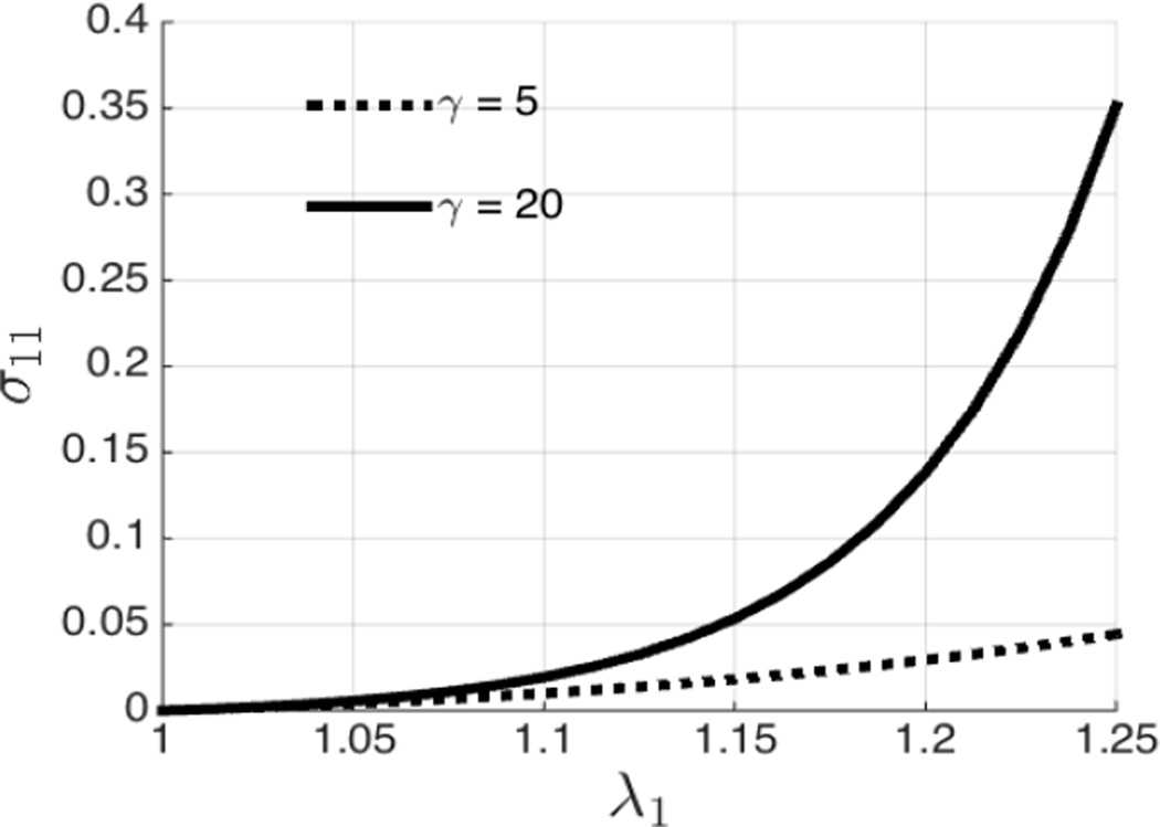
We assume that fibers in the network are not able to sustain compressive loads. In equation (15), this is expressed by including contributions only from those fibers for which λθ ≥ 1.(15) To investigate the predictive capability of our model, the macroscopic constitutive response of a material under uniaxial tension is shown in Figure 2. The two samples considered have the same Young’s modulus E = 1; however they have fibers with different tortuosity, as represented by the different values of γ. We observe that the sample with fibers with smaller tortuosity shows an early onset of nonlinear behavior. This is due to the microstructural differences in the two samples. When we perform a uniaxial tension on a fibrous material, it offers little resistance until a point where embedded fibers become uncoiled, following which they start to carry a significant load causing the stress-strain curve to rise sharply. The fibers with smaller values of tortuosity are recruited at a small value of overall strain and thus that sample displays an early onset of nonlinear behavior.
We note that once a wavy fiber is uncoiled, and it undergoes an increase in stiffness, it may display behavior that is not represented by our model, which assumes that its stiffness keeps increases exponentially. Other types of responses that have been observed beyond this limit include constant stiffness, or a softening due to damage and failure [Shen et al., 2011, Cacho et al., 2007]. This limits the suitability of our microstructural model to levels of microstructural strain where we do not expect any damage. We would like to however point out that the averaging procedure described above, and the inverse problem approach that is described in the following section, is agnostic to this limitation. In particular, the averaging procedure and the inverse problem approach can be applied in conjunction with other microstructural models that demonstrate more accurate large strain response.
Fig. 2.
Macroscopic response of materials comprised of fibers with different tortuosity.
3 The forward problem
In this section we describe a forward elasticity problem for a material whose strain energy density is described by (13). We first pose this problem in three dimensions and then simplify it to the case of two-dimensional plane stress. This latter case is particularly relevant to elasticity imaging using ultrasound and optical techniques, where displacement data is often obtained in a two-dimensional imaging plane.
3.1 Three dimensions
In three dimensions for an incompressible medium, the strong form of the equilibrium equation can be written in the reference configuration Ω0, as
| (16) |
| (17) |
| (18) |
| (19) |
In above equations, F is the deformation gradient, J is its determinant, S is the second Piola-Kirchhoff stress tensor, U is the displacement field, G is the displacement boundary data, H is the applied traction data, and N̂ is a unit outward normal vector. Further, ΓG denotes the part of boundary where the displacements are prescribed (essential BCs), ΓH denotes the portion of the boundary where the tractions are prescribed (natural BCs), and Γ0 denotes the entire boundary of Ω0. For simplicity we assume that any boundary is either an essential or a natural boundary, that is and ΓG ∩ ΓH = ∅.
The equation for the second Piola-Kirchhoff stress tensor is given by
| (20) |
where p is the pressure. Using the expression for the strain energy density given by equation (13) in the above we arrive at
| (21) |
3.2 Plane stress
Under plane stress assumption, the displacements are independent of the out-of-plane coordinate, and all out-of-plane stress components vanish. Using these assumptions in (21), one may eliminate the pressure to arrive at the following relation for Sαβ, which is valid for α, β = 1, 2,
| (22) |
where I2 is the second principal invariant of the two-dimensional right Cauchy-Green tensor. We note that even though macroscopic problem is one of plane-stress, and hence two-dimensional, we assume that the microstructure is still three-dimensional. Consequently the integration above is over two angular coordinates. The equations of equilibrium (16) and the boundary conditions (18) – (19) remain unchanged, with the caveat that they hold in the in-plane coordinates. The equation representing conservation of mass, that is the incompressibility constraint (17), is not enforced explicitly since the out-of-plane deformation adjusts to accommodate it.
The forward problem is given by: Given the material parameters E and γ and the boundary data G and H, determine the displacement field in Ω0 such that equations of equilibrium (16), and the boundary conditions (18) – (19) are satisfied, where the stress tensor is given by (22).
3.3 Variational formulation
In this paper we are interested in solving the inverse problem associated with the forward plane stress problem described in the previous section. In order to do that we will set up an interative scheme, which will require the solution of the forward problem, and the associated adjoint problem at every iteration. We will solve these using the finite element method based on the weak, or the variational, form of the forward problem. This form may be derived from a weighted-residual form of the forward problem, or it may be obtained by minimizing the overall potential energy. In either case, under the plane-stress hypothesis, it is given by: Find the displacement field U ∈ 𝒮 such that,
| (23) |
where
| (24) |
| (25) |
The function spaces 𝒮, and 𝒱 are defined as
| (26) |
| (27) |
Both 𝒮 and 𝒱 spaces are subsets of H1, the Sobolev space of square integrable functions with square integrable derivatives. Functions that are contained in 𝒮 satisfy the Dirichlet boundary condition, while functions in 𝒱 satisfy its homogeneous counterpart.
4 The inverse problem
The inverse problem can be solved as a constrained minimization problem [Gokhale et al., 2008], where the goal is to find the spatial distribution of material properties (E, γ) that minimizes the difference between the measured Ũn and the predicted displacement fields Un, where the superscript n denotes the nth measurement. Each of the predicted displacement fields is required to satisfy the forward elasticity problem described in the previous section.
The objective function is given by
| (28) |
In the equation above the first term represents the displacement matching term that measures the difference between the measured and the predicted displacement fields in the L2 norm. The measured fields are typically obtained by observing the tissue (or the soft material) deform using a conventional imaging modality (like ultrasound, optical coherence tomography, x-ray tomography etc.) and then performing image-cross correlation on successive images in order to determine the incremental displacement field. This incremental field is mapped back to the reference configuration, and then summed in order to obtain the total deformation field.
The predicted displacement fields Un are constrained to satisfy the equations of equilibrium, and are obtained by solving the forward problem corresponding to a given guess of the material property distribution. The “weights” wn that appear in the objective function (28) are selected so that the magnitude of the contribution from multiple measured displacements to the displacement matching term is roughly equal. The tensor T is used to weigh the different components of displacement within a single measurement differently. This is necessary because different components are often measured with different levels of accuracy. For example in ultrasound elastography, the component of the measured displacement along the axis of the transducer is around ten times more accurate than the other components.
The second and the third terms in (28) are the regularization terms, that are added to provide stability to the inverse problem, which is often ill-posed. In particular, it is well known that small perturbations in the measured displacements can lead to large variations in the reconstructed parameters. The regularization term is typically a measure of overall spatial variation of the reconstructed parameters. In our paper we have used the total variation regularization [Rudin et al., 1992],
| (29) |
which penalizes the total variation in the material parameters, without regard to the magnitude of the slope of the variation. In doing so, for sharply varying material properties, it diminishes the contrast of the variation but does not cause it to spread or smear out. We note that in the equation above c is a numerical parameter which ensures that regularization term is smooth function of the material parameters.
The regularization term is multiplied the parameter, α, which is referred to as the regularization parameter. Large values of this parameter enhance the effect of the regularization term at the expense of displacement matching term. This yields smooth material property distributions and large differences between the predicted and the measured displacement fields. Small values of this parameter lead to large variations in the material property distributions but small displacement matching terms. The optimal value of this parameter is dependent on the noise in the measurements, and reflects a compromise between the smoothness of the reconstructed parameters and value of the displacement matching term. One approach to determine this value is to utilize the so-called L-curve [Morozov, 1968]. See [Dong et al., 2016] for an application to the L-curve to a similar problem in computing the spatial distribution of mechanical properties. In this manuscript we have use the L-curve method to obtain the regularization parameters for all cases. Across all cases, the value of this parameter, when non-dimensionalized by the appropriate parameters, was found to vary by about one order of magnitude.
4.1 Solution of the inverse problem
The uniqueness of the solution for the spatial parameters for E and γ has not been demonstrated. However, for a large class of hyperelastic constitutive models with two parameters it has been shown that given two deformation fields: one at small strain, and another at large strain, we are guaranteed a unique solution for the two parameters up to two undetermined constants [Ferreira et al., 2012]. These constants can be determined by knowing these parameters at one point within the domain. We believe that this general approach to proving uniqueness can also be extended to the constitutive model considered in this manuscript, and this will be a topic of future research.
The minimization problem (28) is solved using a quasi-Newton algorithm (the limited-memory BFGS method [Zhu et al., 1997]) that requires the gradient of the objective function with respect to the optimization parameters at every iteration. The gradients are obtained efficiently by using adjoint method [Gokhale et al., 2008, Oberai et al., 2004]. This approach involves the following steps:
Corresponding to each measured displacement field, solve the forward problem to determine the predicted displacement field Un and the stress tensor Sn.
Solve the corresponding adjoint problem in order to determine the adjoint field Wn.
Use the displacement field, the stress tensor and the adjoint field in order to determine the gradient of the objective function with respect to the material parameters using the expressions that appear below.
The derivative of π with respect to the nodal value of the Young’s modulus at node number A, denoted by EA, is given by
where,
| (30) |
where ϕA(X) is the finite element shape function associated with the A-th node. Similarly the expression for the derivative of π with respect to the nodal value of the nonlinear parameter is given by
where
| (31) |
In the followings sections we use the approach described above in order to determine the spatial distribution of material properties of tissue-like specimens from measurements of their interior displacement fields. We first consider “synthetic” or in-silico specimens, where we determine the displacement fields by solving appropriate forward problems. Thereafter we consider physical specimens made from gelatin-agar co-gels and measure the interior displacement field using ultrasound-based elastography methods.
5 Numerical tests with synthetic data
In this section, two-dimensional numerical examples are considered to test the performance of the proposed approach for recovering the spatial distribution of the material parameters. These examples are motivated from inverse problems related to biological applications where one is often looking for inclusions (tumors) whose microstructural properties are significantly different from that of the surrounding tissue.
Problem description
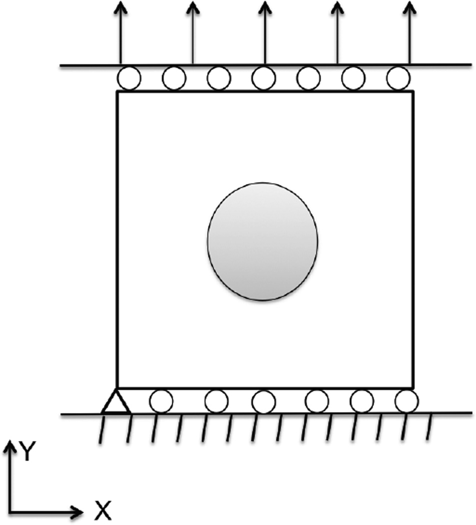
A schematic diagram of the problem setup and boundary conditions are shown in Figure 3. We consider two specimens. Each has dimensions of 10 × 10 units, and consists of an inclusion and a background, where the material properties are shown in Table 1. We note that one specimen has a higher value of Young’s modulus in the inclusion, which could be attributed to a higher concentration of fibers in this region, while the other has higher value of the nonlinear parameter in the inclusion which is attributed to a smaller value of tortuosity in this region.
Fig. 3.
Schematic diagram of the problem setup and boundary conditions.
Table 1.
Material Properties for synthetic Phantoms.
| Parameters | Background | Inclusion | |
|---|---|---|---|
| Specimen 1 | E | 1 | 5 |
| γ | 1 | 1 | |
| Specimen 2 | E | 1 | 1 |
| γ | 1 | 5 | |
The bottom edge is fixed in the vertical direction and traction free in the horizontal direction, whereas the top edge is traction free in the horizontal direction, and uniformly loaded in the vertical direction. The specimen with the contrast in the Young’s modulus is deformed to about 2% strain, and this displacement field is used to reconstruct the Young’s modulus. The specimen with contrast in the nonlinear parameter is deformed to 20% strain, and this displacement field is used to determine the nonlinear parameter. The vertical edges are traction free in both vertical and horizontal directions. In order to prevent rigid body motion, the left corner of the bottom edge is fixed to prevent movement along horizontal direction. The domain is discretized with 10,000 rectangular elements with a total of 10,201 nodes.
To evaluate the performance of the proposed algorithm, displacement fields are generated by solving forward problems with the known material parameters (see Table 1). Then about 0.3%, 1% and 3% white Gaussian noise is added to the displacement fields. These noisy displacement fields are used in the inversion algorithm to recover the material parameter distributions. In both cases, the displacement component along the vertical direction is utilized in the reconstruction.
Results
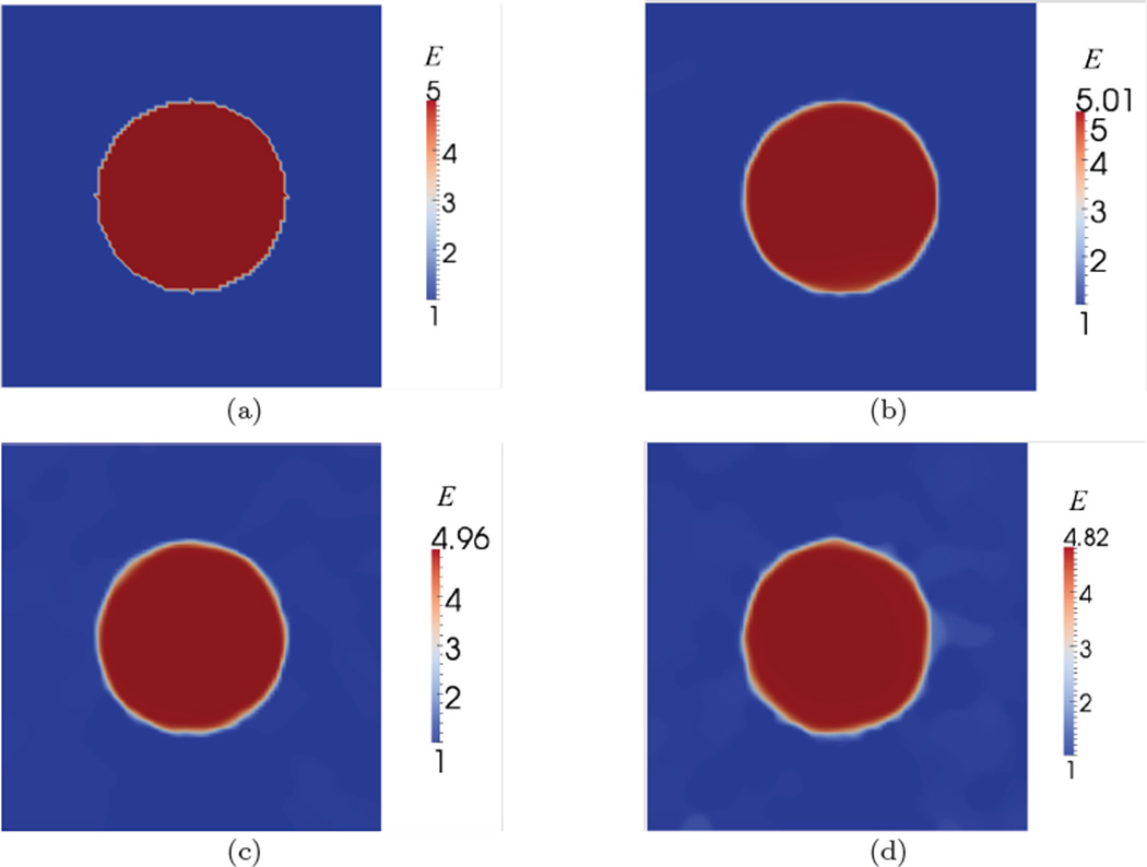
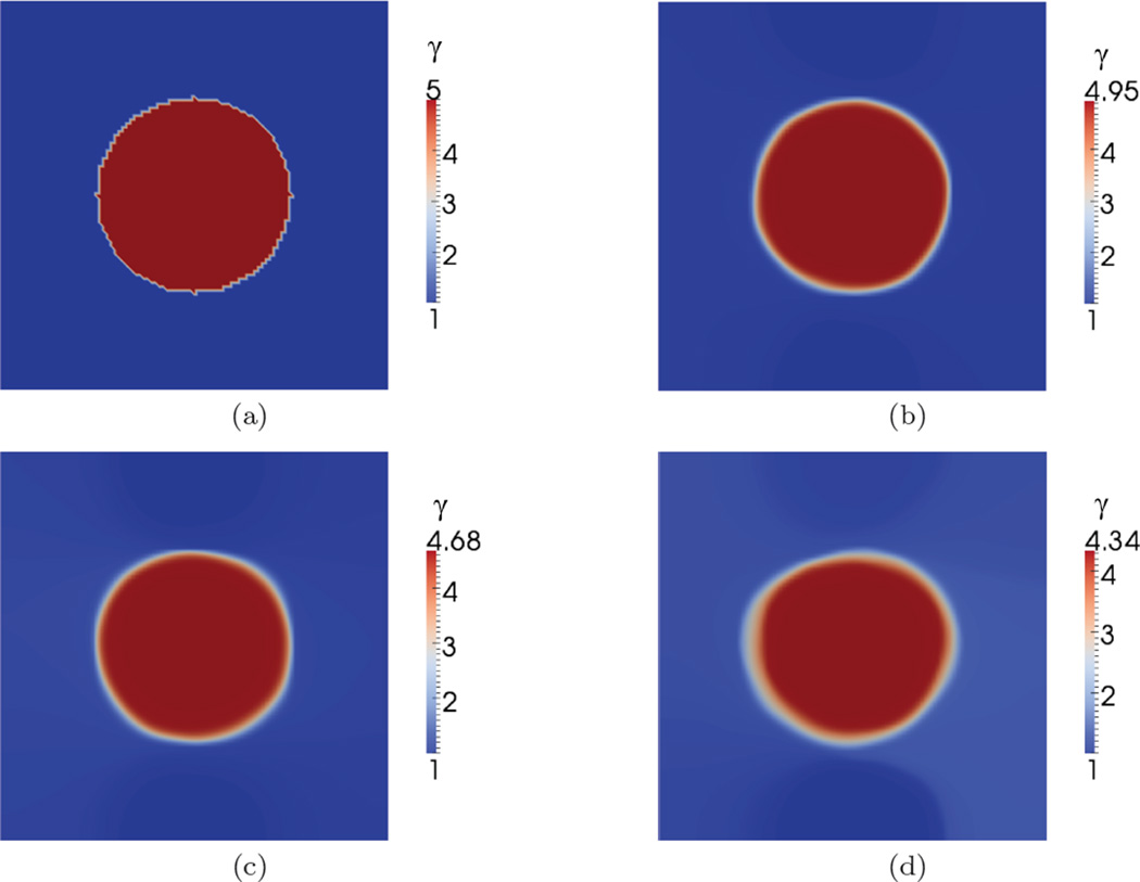
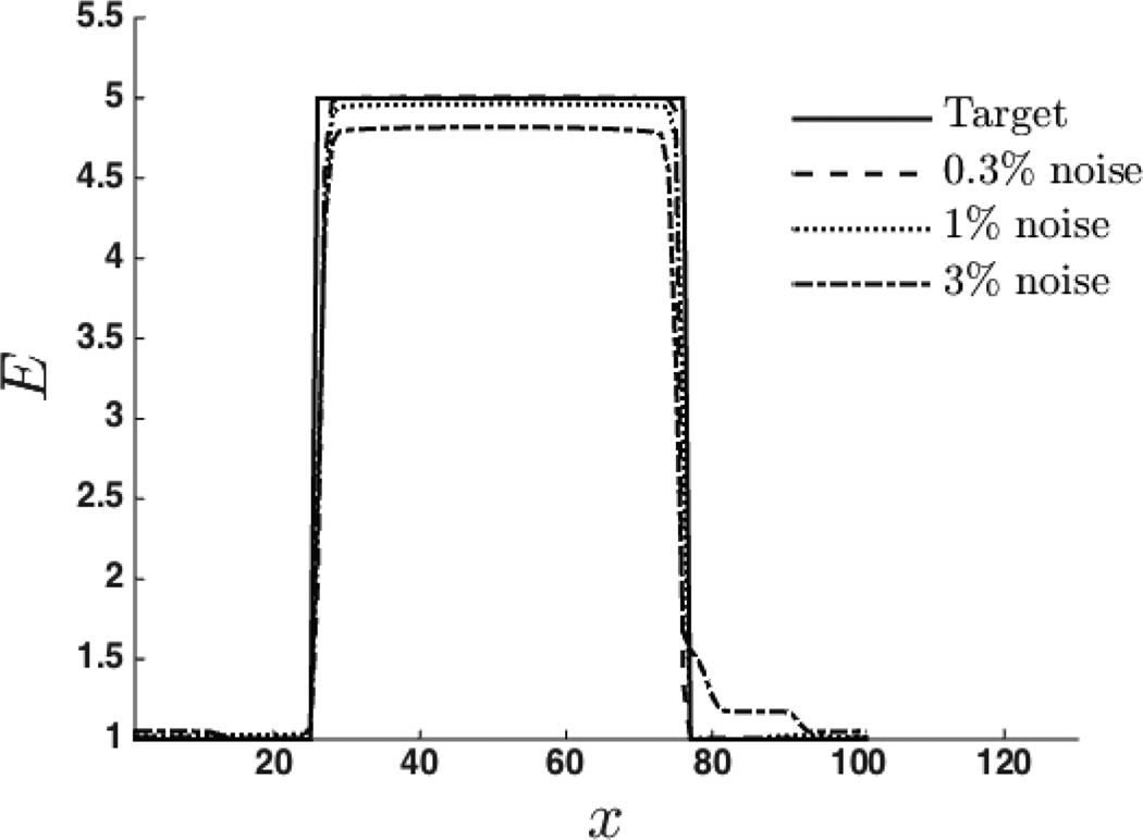
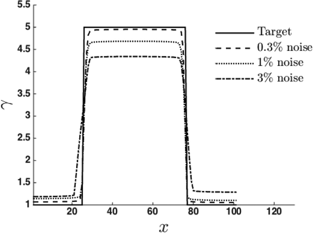
The recovered spatial distribution of material properties, E and γ, are shown in Figure 4 and Figure 6. The values of regularization parameters used for the reconstruction of material properties are shown in Table 2. We observe that the proposed approach is able to capture the inclusions clearly for both specimens. In Figure 5 and Figure 7, we have plotted the exact and the recovered values of E and γ along center line. We note that the reconstructed values are in good agreement with the exact solutions. We also note the effect of the regularization which causes the contrast to diminish with increase values of the regularization parameter.
Fig. 4.
Young’s modulus distributions for Specimen 1. (a) Exact modulus. Reconstructed modulus for data with (b) 0.3%, (c) 1% noise, and (d) 3% noise.
Fig. 6.
Nonlinear parameter (γ) distributions for Specimen 2. (a) Exact parameter. Reconstructed parameter for data with (b) 0.3%, (c) 1% noise, and (d) 3% noise.
Table 2.
Regularization parameters for reconstructions.
| Parameters | 0.3% noise | 1% noise | 3%noise |
|---|---|---|---|
| αE | 1.0e-07 | 3.0e-07 | 8.0e-07 |
| αγ | 1.0e-05 | 5.0e-05 | 1.0e-04 |
Fig. 5.
Young’s modulus E along the center line.
Fig. 7.
Nonlinear parameter γ along the center line.
6 Tissue-mimicking phantom experiments
In this section we utilize displacement data collected from a gelatin-agar tissue-mimicking phantom to validate the performance of our ability to infer the spatial distribution of microstructural properties. The displacement data is obtained by performing image cross-correlation on a sequence of radio-frequency (rf.) ultrasound images as the phantom is slowly compressed.
6.1 Phantom description
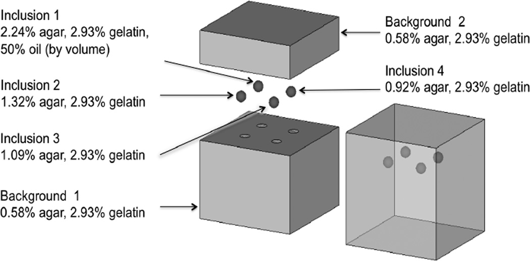
A tissue-mimicking phantom (Figure 8) was fabricated with four stiff spherical inclusions bonded to the background. The methods used to manufacture the phantom are reported in [Pavan et al., 2010, Pavan et al., 2012]. Each of the four spheres and the background contain the same concentration of gelatin (2.93%), but different concentrations of agar, which leads to different microstructure, and consequently, different mechanical properties. The bottom part of the background, which is denoted as “Background 1”, and the upper part, which is denoted as “Background 2”, have the same concentration of gelatin and agar. However, they were manufactured in different batches, and due to the inherent variability in the manufacturing process, they have different mechanical properties. Inclusion 1 contains a dispersion of oil droplets in the gelatin-agar material, which is added to modify its nonlinear mechanical response, as discussed in Section 6.6 and 6.7. The phantom is a cube where each side 100 mm, and the diameter of each inclusion is 10 mm (see Figure 8). The microstructure of hydrated gelatin-agar gels comprises of an interpenetrating network of fibrous links where the concentration of the constituents determines the cross-link density, and therefore, the elastic properties of gel [Clark et al., 1983, Marmorat et al., 2016].
Fig. 8.
A schematic diagram of the tissue-mimicking phantom [Pavan et al., 2012].
6.2 Independent mechanical test
For each component of the phantom (2 backgrounds and 4 inclusions) a separate cylindrical test sample was created at the time of manufacture for independent measurement of the mechanical material properties in a uniaxial compression test. The test is described in [Pavan et al., 2012]. The stress-strain data from this test was then used in conjunction with the uniaxial stress-strain curve of the proposed microstructure-based constitutive model (13) in order to determine the material parameters E and γ. This provides us with an independent measurement of these properties for each component of the phantom (see Table 3). We treat these as the benchmark values in our validation tests.
Table 3.
The composition of the agar, gelatin and oil used to manufacture the phantom and values of material properties E (kPa) and γ measured from independent mechanical tests
| Agar (wt.%) | Gelatin (wt.%) | Oil (vol.%) | E (kPa) | γ | |
|---|---|---|---|---|---|
| Inclusion 1 | 2.24 | 2.93 | 50 | 70 | 3.8 |
| Inclusion 2 | 1.32 | 2.93 | 0 | 145 | 18.5 |
| Inclusion 3 | 1.09 | 2.93 | 0 | 92 | 18.5 |
| Inclusion 4 | 0.92 | 2.93 | 0 | 59 | 20 |
| Background 1 | 0.58 | 2.93 | 0 | 22 | 19 |
| Background 2 | 0.58 | 2.93 | 0 | 28.5 | 15 |
6.3 Elasticity imaging
The phantom was deformed by compressing the top face slowly to about 20% strain. Ultrasound radio-frequency (rf.) echo data was acquired during the compression using a Siemens SONOLINE Antares (Siemens Medical Solutions USA, Inc. Malvern, PA) ultrasound scanner. Displacement fields were estimated between successive pairs of ultrasound images using a modified block matching motion tracking algorithm [Jiang and Hall, 2007]. These were then mapped back to the least deformed state (the reference configuration) and added to yield the accumulated displacement at each compression step. The displacement fields were measured on a 300 × 231 grid (axial by lateral), centered around each inclusion, with a grid spacing of 0.1545 mm × 0.1217 mm.
When solving the inverse problem the imaging plane was assumed to be in a state of plane stress. We note that plane stress is an approximation to the true stress state, which is three-dimensional. However, in ultrasound elasticity imaging the displacement data is obtained in a single plane. As a result it is necessary to reduce a three-dimensional elasticity problem to a two-dimensional problem using either the plane-strain or the plane-stress approximation. Of the two, we believe that plane-stress is appropriate for the given problem. This is because the sample thickness (in the out-of-plane direction) is of the same order as the other dimensions. It is certainly not much greater than the other dimensions, which is a requirement for plane-stress. Further, during the test the sample was unconfined in the out-of-plane direction, and was allowed to expand in that direction. Thus we expect the out-of-plane strain to be non-zero (actually quite significant), which automatically rules out plane strain. Finally, we note that the approach we have developed in this manuscript can be applied to there-dimensional situations whenever data in three dimensions is available.
The measured axial (along the axis of the transducer) displacement was used as prescribed boundary condition in the axial direction on each boundary edge. In the lateral direction, a traction-free condition was assumed on each edge. This was justified based on the lubrication between the compression plate and the phantom, and the fact that the phantom was not confined in any direction.
The inverse problem was solved in a truncated region of interest (ROI) obtained by excluding 39 lines of data from the face close to the ultrasound probe, 8 lines from the opposite face, 9 lines from each lateral face. This was done in order to exclude the noisy displacement measurements close to each of these faces. Further, in order to keep the overall computational costs small, the displacement data was down-sampled by a factor of four in each direction. As a result the reconstructions were performed on a 64 × 54 grid at a resolution of about 0.6180 mm × 0.4869 mm. Due to the fact that the displacement along the axial direction was more accurate than the displacement measured along the lateral direction, only axial displacement was utilized in the reconstructions.
The lower 1/10th of the specimen, which was completely comprised of “Back-ground 1” was treated as a calibration layer. It was assumed that the mechanical and the microstructural properties of this region were known, and these were used to assign quantitative measures to the mechanical and microstructural maps determined for the remainder of specimen. Different approaches were used to calibrate the Young’s modulus (and fiber concentration) and the nonlinear parameters, and these are described in the following sections.
6.4 Young’s modulus
The inverse problem was solved in two steps [Goenezen et al., 2010]. First, the displacement estimate at about 1.5% strain was used to determine the Young’s modulus, while the nonlinear parameter γ was fixed to be a small constant. The initial guess for Young’s modulus was set to 1, and it was constrained to be in the interval (1, 50). The regularization parameter, αE = 1.0e − 05, was selected by performing a sweep and constructing the L-curve.
We note that in the absence of a force measurement the Young’s modulus is determined uniquely up to a multiplicative factor [Tyagi et al., 2014]. In order to compare our reconstructions with the quantitative mechanical measurements, this factor must be determined. This was determined by using the calibration region which is comprised entirely of “Background 1”. The value of the reconstructed Young’s modulus was multiplied by the ratio of the independently measured modulus for Background 1 and the average value of the reconstructed modulus in the calibration layer. The resulting images of the quantitative reconstructed Young’s modulus are shown in Figure 9.
Fig. 9.
Reconstructed spatial distribution of Young’s modulus, E, for agar-gelatin phantoms with four circular inclusions (targets 1 to 4, form left to right).
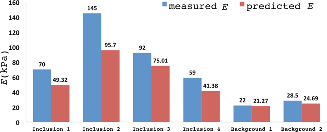
We note that all the inclusions are observed clearly in the Young’s modulus image, where their shapes and boundaries have been accurately reconstructed. We also observe that the top part of the background is stiffer than the bottom part, which is consistent with how the phantom was manufactured. The average values of recovered Young’s modulus (predicted E) for the inclusions and the backgrounds are presented in Figure 10, respectively. Figure 10 also includes the values of Young’s modulus determined from the independent mechanical test (measured E). We note that the trend in the variation of the Young’s modulus of the inclusions is accurately captured in the reconstructed modulus results and error is within 30% in all cases. We also note that contrast in modulus is underestimated in all cases. This is attributed to the effect of the total variation regularization which is known to preserve the sharpness in variations but lower the overall contrast. It may also be attributed to the assumption of plane stress that is used in the reconstructions. Given the geometry of the phantom specimen (see Figure 8) the true state of the specimen is likely to be more complex.
Fig. 10.
Comparison of reconstructed and benchmark Young’s modulus values.
The variations of the modulus in the inclusions is closely related to the concentration of agar. Higher concentration of agar leads to more dense fiber networks, which in turn have a higher average Young’s modulus. A constitutive model that is derived from the microstructure can be used to exploit this link and determine the concentration. This is explored in the following section.
6.5 Fiber concentration
As stated earlier, the microstructure of hydrated gelatin-agar gels is made up from an interpenetrating network of fibrous links where the concentration of the constituents determines the cross-link density, and therefore, the elastic properties of gel [Clark et al., 1983, Marmorat et al., 2016].. It is these cross-links that provide the mechanical strength to the collagen-agar mixture. When the concentration of agar is increased the density of these web-like links increases, and consequently the resulting mixture increases its stiffness. A direct consequence of this is that the homogenized stiffness is determined almost solely by the concentration of agar and not gelatin. This is consistent with the results reported from experiments [Hall et al., 1997] that pure gelatin network is much less stiff when compared with pure agar network.
In our constitutive model this dependence of the Young’s modulus on concentration is captured in (14), where we note that the concentration of agar (n) is proportional to the square root of the Young’s modulus (E). Using this relation, and assuming that the microstructural organization remains the same as the concentration is increased, we may write
| (32) |
Here ncal and Ecal are the agar concentration, and the Young’s modulus of the mixture in the calibration layer, and x is any point in the domain of the specimen. Thus it is possible to use the modulus maps displayed in Figure 9, and the concentration of agar in the calibration layer, in order to create concentration maps displayed in Figure 11. These maps represent the spatial variation of the average concentration of agar within the sample, and within them we can clearly identify the inclusions as regions of higher agar concentration.
Fig. 11.
Reconstructed spatial distribution of agar concentration, n, for gelatin-agar phantoms (targets 2 to 4, from left to right).
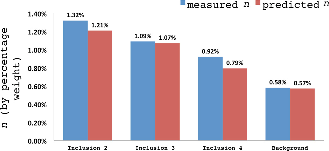
The concentration maps in Figure 11 may be used to compute the average concentration of agar in the two backgrounds and all the inclusions, except inclusion 1, as explained below. These values are reported in Figure 12, where we have also presented the actual agar concentration (measured at the time of manufacture). We note that we are able to accurately capture the trends of agar concentration within all groups of materials and the error in predicting the concentration is about 15%.
Fig. 12.
Comparison of reconstructed and benchmark agar concentration.
We have excluded sample number 1 in our analysis because this sample was created using a mixture of water and oil. The presence of oil droplets in collagen-agar mixture breaks the agar cross-links and completely changes the microstructural organization of the material [Kim et al., 1996, Kim et al., 1999]. In particular it changes the ratio of the number of cross-links to the concentration of agar. Our microstructural model assumes a constant value for this parameter, and therefore cannot be applied in a straightforward manner to this case.
6.6 Nonlinear parameter
In the second step, the displacement data at 20% strain was used to determine the nonlinear parameter, γ, while the Young’s modulus was fixed at the value determined in the first step. The initial guess for γ was 15.5, and it was constrained to be in the interval (1, 100). The regularization parameter, αγ = 1.0e − 05, was selected by performing a sweep and constructing the L-curve. The images of the reconstructed nonlinear parameter are shown in Figure 13.
Fig. 13.
Reconstructed spatial distribution of non-linear parameter, γ, for agar-gelatin phantoms with four circular inclusions (targets 1 to 4, form left to right).
The value of γ in the calibration region (the bottom 1/10th. of the domain) was fixed at the measured value of 19 (measured in an independent mechanical test). The nodal values in this region were not treated as optimization variables while solving the minimization problem.
The recovered images of the nonlinear parameter γ for the phantom are shown in Figure 13. In these images we observe a significant change in the nonlinear parameter for the inclusion in target 1. The inclusions in all other targets appear to have a nonlinear parameter value that is close to the background. We also observe that the images for the nonlinear parameter are noisier than those for the Young’s modulus. We believe that this is the case because the level of strain applied in this test is barely sufficient to resolve the contrast in the nonlinear properties the samples.
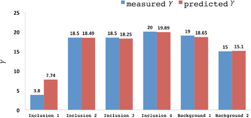
The average value of the nonlinear parameter for the background and the inclusions are shown in Figure 14, where they are compared with the values determined from an independent numerical test. We observe that we predict the trends correctly; however we incur significant error when the value of γ is small. This is to be expected since it would take very large values of strain to observe differences in material behavior when the value of γ is small.
Fig. 14.
Comparison of reconstructed and benchmark nonlinear parameter.
From the nonlinear parameter images, we observe that there is one inclusion in target 1, and there are no inclusions in target 2 to 4, which is consistent with the fact that the inclusions and background for target 2, 3, 4 were manufactured to have the same nonlinear parameter, and inclusion 1 has distinct nonlinear parameter from the background. The change in macroscopic mechanical behavior is due to a difference in the microstructure as described in the following section.
6.7 Fiber tortuosity
Once the value of γ is known, it can be used in conjunction with (3) to determine the value of tortuosity of the fibers. These images are plotted in Figure 15 for C = e.
Fig. 15.
Reconstructed spatial distribution of fiber tortuosity, τ, for agar-gelatin phantoms with four circular inclusions (targets 1 to 4, form left to right).
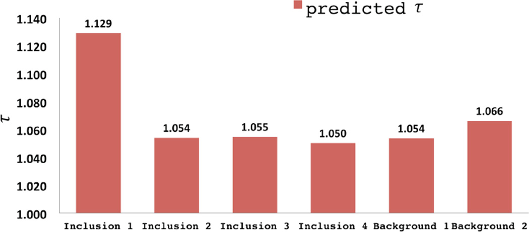
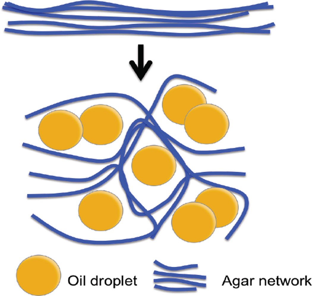
Here we observe a significant difference only for the inclusion in target 1. This is the inclusion that is manufactured with 50% by volume oil. It is well known that the oil disperses within the gel as tiny droplets, and that the agar-gelatin network bends around these droplets [Kim et al., 1999]. This increases the overall tortuosity of the network, and is likely responsible for the higher value of tortuosity that we observe. Whether this is really the case can only be confirmed through scanning electron microscope (SEM) images of the specimen, which are unavailable. We note further that these parameters are to be interpreted as lower bounds on the tortuosity. With 12% axial compression, we induce approximately 6% maximum tensile strain in the specimen, which occurs in the lateral directions. At these stretch levels, we would not be able to observe contributions from fibers of tortuosity larger than about 1.06.
7 Conclusions
In this paper we considered an extension to elasticity imaging wherein the constitutive model was derived from microstructural considerations. In particular, a microstructure comprised of a network of elastic fibers was assumed and the constitutive model was obtained from a simple homogenization procedure. Consequently, the parameters that appear in this model were directly linked to local averages of microstructural quantities such as fiber concentration, initial fiber stiffness and fiber tortuosity. This constitutive equation was used in conjunction with the equations of equilibrium to solve the inverse elasticity problem: given the displacement field in the interior of a specimen, determine the spatial distribution of the material parameters, and hence the spatial distribution of the local averages of the microstructural parameters, within the specimen. An efficient computational strategy was developed and implemented to solve this challenging inverse problem. The performance of this strategy was tested on in-silico tissue samples. Thereafter this approach was used to infer the spatial distribution of the microstructural properties of agar-gelatin co-gels. It was found that it accurately predicted the spatial distribution of agar fiber concentration, and provided physically consistent spatial distributions of fiber tortuosity.
While the approach described in this manuscript has demonstrated the viability of determining the spatial distribution of microstructural parameters from the macroscopic mechanical response of soft material, there are several areas that are open to further exploration. First, the uniqueness of the inverse problem for the class of constitutive laws used in this manuscript can be worked out. Second, other constitutive laws for the microstructure that are valid when the fibers are fully stretched and even start to incur damage, may be considered. Third, a study designed to quantitatively validate the performance of the proposed method in determining fiber tortuosity is called for. In this study the nonlinear parameter and the tortuosity would be determined in the way described in this manuscript. However, this step will be followed by an independent evaluation of the specimen microstructure using techniques such as scanning electron microscopy (SEM) or second harmonic generation (SHG) imaging. Finally, the application of these methods to in-vivo tissue data in order to determine microstructural changes in diseased tissue is a potential area of application in medical diagnosis.
Fig. 16.
Reconstructed values of fiber tortuosity, τ.
Fig. 17.
Schematic diagram of the effect of oil droplets embedded in gelatin-agar gel.
Acknowledgments
Support from the NIH (NCI-R01CA100373 and NCI-R01CA140271) and the NSF (Grant Nos. 1148124 and 1148111) is acknowledged.
A
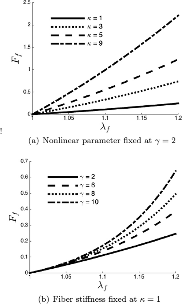
We examine the effect of the parameter κ and nonlinear parameter γ on the force-stretch response of individual fibers to better understand the relevance of these parameters. In Figure 18(a) we have plotted force-stretch curves for a family of fibers where the nonlinear parameter γ is fixed at 2 and the fiber stiffness κ is varied from 1 to 9. We notice that the slope of curves at small strain increases as the value of fiber stiffness increases indicating that κ determines the small strain behavior of individual fibers. In Figure 18(b) we have plotted force-stretch curves for fibers that have the same fiber stiffness, κ = 1, but different and values of the nonlinear parameter γ ∈ (2, 10). We observe that the fibers show an increase in stiffness with increasing strain at all values of γ. However, with increasing γ, the onset of the this increase shifts to lower values of stretch. This behavior can be used to link the nonlinear parameter γ directly to the tortuosity of the fibers as described in the following paragraph.
Fig. 18.
Force-stretch curve for a single fiber. (a) Increasing the fiber stiffness increases the slope of the force-stretch curves at small strain.(b) As the nonlinear parameter γ is increased, the fiber becomes nonlinear at smaller strains.
B
For an incompressible material in uniaxial tension, the axial component of the Second Piola-Kirchhoff stress is given by
| (33) |
where λθ is stretch of an individual fiber, and θ = [γ, ϕ] determines its orientation. For an incompressible material in uniaxial tension, the stretch of each fiber is related to the macroscopic stretch, λ1, through the relation
| (34) |
Now assuming that the strain is small, that is λ1 = 1 + ε11, where |ε11| ≪ 1, we arrive at
| (35) |
Using this expression in (33) and recognizing that |ε11| ≪ 1,
| (36) |
We further assume that the fibers carry load only in tension, that is for values of θ in (35) for which λθ > 1. This implies that the integral in (36) must be evaluated within the limits , which yields
Recognizing that under the small strain assumption, the second PK stress tensor and the Caucy stress tensor reduce to the same expression, the Young’s modulus is given by
Contributor Information
Tengxiao Liu, Scientific Computation Research Center, Rensselaer Polytechnic Institute, Troy, NY, USA, Tel.: (518) 276-6795, liut5@rpi.edu.
Timothy J. Hall, Medical Physics, University of Wisconsin, Madison, WI, USA, Tel.: (608)265-9459, tjhall@wisc.edu
Paul E. Barbone, Mechanical Engineering, Boston University, Boston, MA, USA, Tel.: (617) 353-6063, barbone@bu.edu
Assad A. Oberai, Scientific Computation Research Center, Rensselaer Polytechnic Institute, Troy, NY, USA, Tel.: (518)276-3386, oberaa@rpi.edu
References
- Alastrué V, Martinez M, Doblaré M, Menzel A. Anisotropic micro-sphere-based finite elasticity applied to blood vessel modelling. Journal of the Mechanics and Physics of Solids. 2009;57(1):178–203. [Google Scholar]
- Barbone P, Oberai A. A Review of the Mathematical and Computational Foundations of Biomechanical Imaging. Computational Modeling in Biomechanics. 2010:375–408. [Google Scholar]
- Bažant P, Oh B. Efficient numerical integration on the surface of a sphere. ZAMM-Journal of Applied Mathematics and Mechanics/Zeitschrift für Angewandte Mathematik und Mechanik. 1986;66(1):37–49. [Google Scholar]
- Berg WA, Cosgrove DO, Doré CJ, Schäfer FK, Svensson WE, Hooley RJ, Ohlinger R, Mendelson EB, Balu-Maestro C, Locatelli M, et al. Shear-wave elastography improves the specificity of breast us: the be1 multinational study of 939 masses. Radiology. 2012;262(2):435–449. doi: 10.1148/radiol.11110640. [DOI] [PubMed] [Google Scholar]
- Billiar KL, Sacks MS. A Method to Quantify the Fiber Kinematics of Planar Tissues under Biaxial Stretch. Journal of Biomechanics. 1997;30:753–756. doi: 10.1016/s0021-9290(97)00019-5. [DOI] [PubMed] [Google Scholar]
- Billiar KL, Sacks MS. Biaxial Mechanical Properties of the Native and Glutaraldehyde-treated Aortic Valve Cusp: Part ii - A Structural Constitutive Model. Journal of Biomechanical Engineering-Transactions of the Asme. 2000a;122:327–335. doi: 10.1115/1.1287158. [DOI] [PubMed] [Google Scholar]
- Billiar KL, Sacks MS. Biaxial Mechanical Properties of the Natural and Glutaraldehyde Treated Aortic Valve Cusp - Part i: Experimental Results. Journal of Biomechanical Engineering-Transactions of the Asme. 2000b;122:23–30. doi: 10.1115/1.429624. [DOI] [PubMed] [Google Scholar]
- Broedersz CP, Sheinman M, Mackintosh FC. Filament-length-controlled Elasticity in 3d Fiber Networks. Physical Review Letters. 2012;108:078102. doi: 10.1103/PhysRevLett.108.078102. [DOI] [PubMed] [Google Scholar]
- Cacho F, Elbischger PJ, Rodriguez JF, Doblare M, Holzapfel GA. A Constitutive Model for Fibrous Tissues Considering Collagen Fiber Crimp. International Journal of Non-Linear Mechanics. 2007;42(2):391–402. [Google Scholar]
- Clark AH, Richardson RK, Ross-Murphy SB, Stubbs JM. Structural and mechanical properties of agar/gelatin co-gels. small-deformation studies. Macromolecules. 1983;16:1367–1374. [Google Scholar]
- Dong L, Wijesinghe P, Dantuono JT, Sampson DD, Munro PR, Kennedy BF, Oberai AA. Quantitative compression optical coherence elastography as an inverse elasticity problem. IEEE Journal of Selected Topics in Quantum Electronics. 2016;22(3):1–11. [Google Scholar]
- Ferreira E, Oberai A, Barbone P. Uniqueness of the elastography inverse problem for incompressible nonlinear planar hyperelasticity. Inverse Problems. 2012;28(6):065008. [Google Scholar]
- Ferry JD. Mechanical Properties of Substances of High Molecular Weight. iv. Rigidities of Gelatin Gels; Dependence on Concentration, Temperature and Molecular Weight. Journal of the American Chemical Society. 1968;70:2244–2249. doi: 10.1021/ja01186a074. [DOI] [PubMed] [Google Scholar]
- Garikipati K, Göktepe S, Miehe C. Elastica-based strain energy functions for soft biological tissue. Journal of the Mechanics and Physics of Solids. 2008;56(4):1693–1713. [Google Scholar]
- Gasser TC, Ogden RW, Holzapfel A. Hyperelastic modelling of arterial layers with distributed collagen fibre orientations. J R Soc Interface. 2006;3(6):15–35. doi: 10.1098/rsif.2005.0073. [DOI] [PMC free article] [PubMed] [Google Scholar]
- Goenezen S, Barbone PE, Oberai AA. Solution of the Nonlinear Elasticity Imaging Inverse Problem: the Incompressible Case. Computer Methods in Applied Mechanics and Engineering. 2010 doi: 10.1016/j.cma.2010.12.018. [DOI] [PMC free article] [PubMed] [Google Scholar]
- Goenezen S, Dord JF, Sink Z, Barbone PE, Jiang J, Hall TJ, Oberai AA. Linear and Nonlinear Elastic Modulus Imaging: An Application to Breast Cancer Diagnosis. Medical Imaging, IEEE Transactions on. 2012;31(8):1628–1637. doi: 10.1109/TMI.2012.2201497. [DOI] [PMC free article] [PubMed] [Google Scholar]
- Gokhale NH, Barbone PE, Oberai AA. Solution of the Nonlinear Elasticity Imaging Inverse Problem: the Compressible Case. Inverse Problems. 2008;24:045010. [Google Scholar]
- Hall TJ, Bilgen M, Insana MF, Krouskop TA. Phantom Materials for Elastography. IEEE Transactions on Ultrasonics Ferroelectrics and Frequency Control. 1997;44:1355–1365. [Google Scholar]
- Head DA, Levine AJ, MacKintosh FC. Deformation of Cross-linked Semiexible Polymer Networks. Physical Review Letters. 2003a;91:108102. doi: 10.1103/PhysRevLett.91.108102. [DOI] [PubMed] [Google Scholar]
- Head DA, Levine AJ, MacKintosh FC. Distinct Regimes of Elastic Response and Deformation Modes of Cross-linked Cytoskeletal and Semiexible Polymer Networks. Physical Review E. 2003b;68:061907. doi: 10.1103/PhysRevE.68.061907. [DOI] [PubMed] [Google Scholar]
- Huisman EM, Lubensky TC. Internal Stresses, Normal Modes, and Nonaffinity in Three-dimensional Biopolymer Networks. Physical Review Letters. 2011;106:088301. doi: 10.1103/PhysRevLett.106.088301. [DOI] [PubMed] [Google Scholar]
- Huwart L, Sempoux C, Vicaut E, Salameh N, Annet L, Danse E, Peeters F, ter Beek L, Rahier J, Sinkus R, Horsmans Y, Beers B. Magnetic resonance elastography for the noninvasive staging of liver fibrosis. Gastroenterology. 2008;135(1):32–40. doi: 10.1053/j.gastro.2008.03.076. [DOI] [PubMed] [Google Scholar]
- Jiang J, Hall TJ. A Parallelizable Real-time Ultrasonic Speckle Tracking Algorithm with Applications to Ultrasonic Strain Imaging. Physics in Medicine and Biology. 2007;52:3773–3790. doi: 10.1088/0031-9155/52/13/008. [DOI] [PubMed] [Google Scholar]
- Kass L, Erler J, Dembo M, Weaver V. Mammary epithelial cell: inuence of extracellular matrix composition and organization during development and tumorigenesis. International Journal of Biochemistry and Cell Biology. 2007;39(11):1987–1994. doi: 10.1016/j.biocel.2007.06.025. [DOI] [PMC free article] [PubMed] [Google Scholar]
- Kim KH, Gohtani S, Matsuno R, Yamano Y. Effects of Oil Droplet and Agar Concentration on Gel Strength and Microstructure of o/w Emulsion Gel. Journal of Texture Studies. 1999;30:319–335. [Google Scholar]
- Kim KH, Gohtani S, Yamano Y. Effects of Oil Droplets on Physical and Sensory Properties of o/w Emulsion Agar Gel. Journal of Texture Studies. 1996;27:655–670. [Google Scholar]
- Lanir Y. A Structural Theory for the Homogeneous Biaxial Stress-strain Relationship in Flat Collagenous Tissues. Journal of Biomechanics. 1979;12:423–436. doi: 10.1016/0021-9290(79)90027-7. [DOI] [PubMed] [Google Scholar]
- Lanir Y. Constitutive Equations for Fibrous Connective Tissues. Journal of Biomechanics. 1983;16:1–12. doi: 10.1016/0021-9290(83)90041-6. [DOI] [PubMed] [Google Scholar]
- Liu J, Koenderink GH, Kasza KE, Mackintosh FC, Weitz DA. Visualizing the Strain Field in Semiexible Polymer Networks: Strain Fluctuations and Nonlinear Rheology of F-actin Gels. Physical Review Letters. 2007;98:198304. doi: 10.1103/PhysRevLett.98.198304. [DOI] [PubMed] [Google Scholar]
- Marmorat C, Arinstein A, Koifman N, Talmon Y, Zussman E, Rafailovich M. Cryo-imaging of hydrogels supermolecular structure. Scientific reports. 2016:6. doi: 10.1038/srep25495. [DOI] [PMC free article] [PubMed] [Google Scholar]
- Miehe C, Schröder J, Becker M. Computational homogenization analysis in finite elasticity: material and structural instabilities on the micro-and macro-scales of periodic composites and their interaction. Computer Methods in Applied Mechanics and Engineering. 2002;191(44):4971–5005. [Google Scholar]
- Morozov VA. The Error Principle in the Solution of Operator Equations by the Regularization Method. USSR Computational Mathematics and Mathematical Physics. 1968;8:63–87. [Google Scholar]
- Oberai AA, Gokhale NH, Doyley MM, Bamber JC. Evaluation of the Adjoint Equation Based Algorithm for Elasticity Imaging. Physics in Medicine and Biology. 2004;49:2955–2974. doi: 10.1088/0031-9155/49/13/013. [DOI] [PubMed] [Google Scholar]
- Ophir J, Cespedes I, Ponnekanti H, Yazdi Y, Li X. Elastography - A Quantitative Method for Imaging the Elasticity of Biological Tissues. Ultrasonic Imaging. 1991;13:111–134. doi: 10.1177/016173469101300201. [DOI] [PubMed] [Google Scholar]
- Parker K, Taylor L, Gracewski S, Rubens D. A unified view of imaging the elastic properties of tissue. The Journal of the Acoustical Society of America. 2005;117:2705. doi: 10.1121/1.1880772. [DOI] [PubMed] [Google Scholar]
- Pavan TZ, Madsen EL, Frank GR, Carneiro AA, Hall TJ. Nonlinear elastic behavior of phantom materials for elastography. Physics in Medicine and Biology. 2010;55:2679–2692. doi: 10.1088/0031-9155/55/9/017. [DOI] [PMC free article] [PubMed] [Google Scholar]
- Pavan TZ, Madsen EL, Frank GR, Jiang J, Carneiro AA, Hall TJ. A nonlinear elasticity phantom containing spherical inclusions. Physics in Medicine and Biology. 2012;57:4787–4804. doi: 10.1088/0031-9155/57/15/4787. [DOI] [PMC free article] [PubMed] [Google Scholar]
- Provenzano PP, Eliceiri KW, Campbell JM, Inman DR, White JG, Keely PJ. Collagen reorganization at the tumor-stromal interface facilitates local invasion. BMC medicine. 2006;4(1):38. doi: 10.1186/1741-7015-4-38. [DOI] [PMC free article] [PubMed] [Google Scholar]
- Rudin L, Osher S, Fatemi E. Nonlinear total variation based noise removal algorithms. Physica D. Nonlinear Phenomena. 1992;60(1–4):259–268. [Google Scholar]
- Shahsavari A, Picu RC. Model Selection for Athermal Cross-linked Fiber Networks. Physical Review E. 2012;86:011923. doi: 10.1103/PhysRevE.86.011923. [DOI] [PubMed] [Google Scholar]
- Shen ZL, Kahn H, Ballarini R, Eppell SJ. Viscoelastic properties of isolated collagen fibrils. Biophysical journal. 2011;100(12):3008–3015. doi: 10.1016/j.bpj.2011.04.052. [DOI] [PMC free article] [PubMed] [Google Scholar]
- Talwalkar JA, Kurtz D, Schoenleber S, West C, Montori V. Ultrasound-based transient elastography for the detection of hepatic fibrosis: systematic review and meta-analysis. Clin. Gastroenterol. Hepatol. 2007;5(10):1214–1220. doi: 10.1016/j.cgh.2007.07.020. [DOI] [PubMed] [Google Scholar]
- Tyagi M, Goenezen S, Barbone PE, Oberai AA. Algorithms for Quantitative Quasi-static Elasticity Imaging Using Force Data. International Journal for Numerical Methods in Biomedical Engineering. 2014;30:1421–1436. doi: 10.1002/cnm.2665. [DOI] [PMC free article] [PubMed] [Google Scholar]
- Wells RG. Tissue Mechanics and Fibrosis. Biochimica et Biophysica Acta. 2013;1832:884–890. doi: 10.1016/j.bbadis.2013.02.007. [DOI] [PMC free article] [PubMed] [Google Scholar]
- Wilhelm J, Frey E. Elasticity of Stiff Polymer Networks. Physical Review Letters. 2003;91:108103. doi: 10.1103/PhysRevLett.91.108103. [DOI] [PubMed] [Google Scholar]
- Zhu C, Byrd R, Nocedal J. L-BFGS-B: Algorithm 778: L-BFGS-B, FORTRAN routines for large scale bound constrained optimization. ACM Transactions on Mathematical Software. 1997;23(4):550–560. [Google Scholar]
- Zulliger MA, Fridez P, Hayashi K, Stergiopulos N. A Strain Energy Function for Arteries Accounting for Wall Composition and Structure. Journal of Biomechanics. 2004;37:989–1000. doi: 10.1016/j.jbiomech.2003.11.026. [DOI] [PubMed] [Google Scholar]


