Incorporation of Hierarchical Structure into EPP Fitting with Examples of Estimating Sub-National HIV/AIDS Dynamics

Abstract

Objectives

This article aims to give Spectrum/EPP users and the scientific community a basic understanding of the underlying statistical model used to incorporate hierarchical structure in HIV sub-national estimation, and to show how it has been implemented in the Spectrum/ Estimation and Projection Package (EPP) interface for improving sub-epidemic estimation. The article also provides recommended default settings for this new model.

Methods

We apply a generalized linear mixed effects model (GLMM) on ANC prevalence data to get area-specific prevalence and uncertainty estimates, and transform those estimates to auxiliary data. We then fit the EPP model to both the observed data and auxiliary data.

Results

We apply the proposed methods to four countries with different levels of data availability. We compare the out-of-sample prediction accuracy of the proposed method with varying auxiliary sample sizes and EPP without auxiliary data.

Conclusion

We find that borrowing information from data-rich areas to data-sparse areas using our proposed method improves EPP fit in data-sparse areas. We recommend using the sample size estimated from GLMM as the default auxiliary sample size.

1. Introduction

Every day roughly 5,700 people are newly infected with HIV according to UNAIDS 2016 estimates [1]. The location and the characteristics of the people who are newly infected with HIV provide critical information for country programme managers to develop effective and efficient responses. Good understanding of epidemics at sub-national levels allows managers to re-allocate resources and respond more precisely and effectively to emerging epidemics.

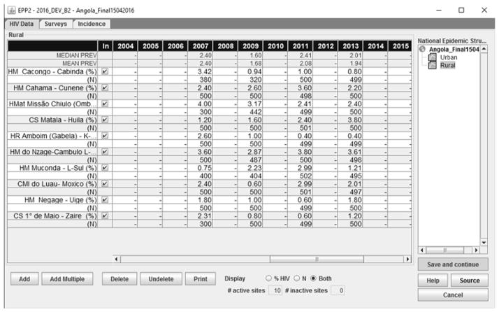
The most informative data source for monitoring an epidemic is incidence data, often measured as the proportion of recently infected individuals among the uninfected population of interest. However, determining whether an individual is recently infected by HIV is more difficult than determining whether an individual is HIV positive. Therefore, the prevalence data from surveillance systems, e.g., such as antenatal clinics (ANC) sites or cross-sectional surveys that include HIV testing among key populations, are the main data sources for estimating HIV epidemics. Figure 1 gives an example of the ANC prevalence data from the rural area of Angola with multiple surveillance sites (screenshot from the Spectrum software used by UNAIDS for constructing global, national and sub-national estimates). At each year and each site, the sample size and the percentage of HIV+ individuals are recorded.

Figure 1.

ANC prevalence data in Rural Angola

When epidemiological data cannot be directly observed, mathematical models are used to estimate the new infections as well as AIDS deaths and other quantities that are not easily available through surveillance systems in low resource settings [2]. In recent years, UNAIDS and partners have been investigating models that provide a more detailed geographic understanding of the HIV epidemic. These models require extensive data at sub-national levels. In many countries, the detailed data are available only for limited areas and years. In regions where data are sparse, estimating the epidemic based merely on the data gathered within those regions will lead to unreliable and highly uncertain results. Figure 2 shows an example of fitting the EPP model in the Spectrum/EPP fitting engine to the ANC data (black dots) in the rural and the urban areas of Angola. The black curve is the posterior median of the estimated prevalence trend and the shaded area represents the uncertainty bounds around the median. We can see that in the rural area we do not have any ANC data until 2007, which leads to high uncertainty about the early period trend such as when the epidemic started and when it peaked.

Figure 2.

The EPP model fitted to Angola rural (left) and urban (right) datasets. The black dots are ANC data. The black curve is the posterior median of the prevalence and the shaded area represents the uncertainty bounds.

To improve the estimation in the data sparse areas like Angola Rural, one option is to “borrow” data from other areas like Angola Urban. It is reasonable to assume some similarities in the epidemic trends among areas within the same country. For example, in Urban Angola with observations in the early 2000’s, we estimate the epidemic started in the 1990’s and peaked after 2000. If we can incorporate such information into the rural area estimation, it may reduce the uncertainty in the rural area’s early epidemic and improve the overall trend estimation.

Bao et. al. [4] introduce the idea of sharing information across sub-epidemics (regions or high-risk groups) of a country in a hierarchical model, and creating one auxiliary data set for each sub-epidemic with prevalence and sample size estimates from the hierarchical model. For EPP fitting purposes this auxiliary data then serves as an additional site that transfers information from other regions; for simplicity this will be referred to as a pseudo-site in the software itself. EPP model is then fitted to both the actually observed data and the auxiliary data to estimate prevalence, incidence, and mortality for each area. Bao et. al. [4] apply their method to two countries as illustrative examples. The detailed implementation and connection with the UNAIDS supported software (Spectrum/EPP) are not discussed.

In this paper, we apply the Bao et. al. [4] approach to four countries with different data availability to demonstrate its varying degree of improvement over the original EPP model. We discuss in detail the implementation of the method and its interface with Spectrum/EPP. We investigate the effects of the sample size assigned to the auxiliary prevalence data points. Finally, we recommend default settings for Spectrum/EPP users. This new model is being incorporated into Spectrum/EPP 2017.

2. Method

In this section, we introduce the hierarchical model used for joint modelling of prevalence data from multiple areas, explain the mechanism of incorporating the hierarchical structure via auxiliary data, and describe the procedure of utilizing the hierarchical model in Spectrum/EPP software.

2.1. Generalized Linear Mixed Model

The available data are observed prevalence rates at ANC sites in different areas. For each country, there are multiple areas, defined either by geographic regions or as urban and rural. Within each area, there are multiple observation sites. Due to the structure of the data, it is possible to use a hierarchical modeling framework to describe the relationships among different layers of the data. Bao et. al. [4] propose a generalized linear mixed effect model (GLMM) for the prevalence data as follows:

$$\begin{array}{c}{Y}_{\mathit{ait}}~\text{Binomial}(n_{\mathit{ait}},{\rho }_{\mathit{ait}}),\\ \text{logit}({\rho }_{\mathit{ait}})={\beta }_0+f(t)+b_a+f_a(t)+b_{i(a)},\end{array}$$ (1)

where Y_ait is the observed HIV+ cases in area a, clinic i, at time t, n_ait and ρ_ait are the corresponding clinic size and prevalence rate, f(t) is the country-level flexible time trend, such as splines, b_a is the area-level random intercept, b_i(a) is the clinic-level random intercept nested within a specific area, and f_a(t) is the area-specific random time trend which implies that each area’s time trend borrows some information from other areas.

One property of the binomial distribution is that the mean of the response Y is n × ρ and the variance has to be n × ρ × (1 − ρ). In real data, the situation that the mean and variance of the binomial outcome do not satisfy this relationship is called over-dispersion. To account for the additional dispersion parameter, one popular choice is a Beta-Binomial model, which allows the probability ρ to be a random variable from a Beta distribution. This additional hierarchical structure results in an over-dispersion parameter that measures the pairwise correlation between the observations within each clinic. When there is indeed some correlation among the samples within each site, the Beta-Binomial model describes the data pattern in a more accurate way. If this over-dispersion parameter is very small, the Beta-Binomial distribution behaves similarly to a Binomial distribution, which implies that the samples are independent and the over-dispersion is negligible.

In this manuscript, we offer the Beta-Binomial model as an alternative to the Binomial model proposed in Bao et. al. [4]. We check the fitted over-dispersion parameter of the Beta-Binomial model and diagnostic plots of the Binomial model to decide which model to use. We then use the selected model to generate the prevalence trend estimates for each area.

2.2. Incorporating GLMM into EPP

As discussed in the Introduction, to estimate the unobserved incidence rates and AIDS deaths, we need to utilize a mathematical model grounded in the transmission and progression dynamics of HIV. Spectrum/EPP, which is used by most countries to develop HIV estimates, is based on the following Susceptible-Infected (SI) model for the age 15–49 adult population:

$$\{\begin{array}{l}\frac{dZ(t)}{dt}=E(t)-r(t)\rho (t)Z(t)-\mu (t)Z(t)-a_{50}(t)Z(t)+M(t)Z(t),\hfill \\ \frac{dY(t)}{dt}=r(t)\rho (t)Z(t)-\text{HIVdeath}(t)-a_{50}(t)Y(t)+M(t)Y(t).\hfill \end{array}$$ (2)

In (2), at time t, Z(t) is the susceptible population, Y(t) is the infected population, E(t) is the number of people entering the population (who just turned 15), r(t) is the infection rate, ρ(t) is the prevalence rate, μ(t) is the non-HIV death rate, a₅₀(t) is the population exit rate (who just turned 50), M(t) is the rate of net migration into the population, and HIVdeath(t) is the number of deaths in the infected population, which is calculated using a CD4 progression model [7]. Equation (2) is a dynamic system that calculates the HIV infections in the population. Given an initial value, the system generates a series of prevalence rates, incidence rates, and HIV mortality rates. The output prevalence of System (2), ρ(t), is then linked to the observed prevalence data and population survey data through a linear mixed effects model as follows:

$$\begin{array}{ccc}{W}_{it}& =& {\mathrm{\Phi }}^{-1}({\rho }_t)+\alpha +b_i+{\epsilon }_{it},\\ b_i& ~& N(0,{\sigma }^2),\\ {\epsilon }_{it}& ~& N(0,v_{it}),\end{array}$$ (3)

where $W_{it}={\mathrm{\Phi }}^{-1}(\frac{Y_{it}+0.5}{N_{it}+1})$, Φ⁻¹ is the inverse cumulative distribution function of the standard normal distribution, α is the bias of ANC data with respect to prevalence data from national population-based household surveys (NPBS), b_i is the site-specific random effect, σ² is assumed to have an inverse-Gamma prior which gets integrated out in the likelihood evaluation, and v_it is a fixed quantity that depends on the clinic data and approximates the binomial variation. The shape of the prevalence curve is mainly determined by System (2) and ANC data, while the level of the prevalence needs to calibrate to the NPBS level as in Model (3). More details can be found in [8] and [9].

We adopt the framework of Bao et. al. [4] to incorporate the GLMM results as auxiliary data into the EPP model. For each area, we create a pseudo-site with the prevalence and sample size derived from the predictive distribution of the area prevalence estimated from GLMM. Specifically, let μ_at and v_at be the posterior mean and variance of the prevalence in area a and year t. From the Binomial mean and variance relationship, the GLMM estimated sample size of this pseudo-site can be calculated by μ_at(1 − μ_at)/v_at. The pseudo-site can be viewed as prior information of the area epidemic. The sample size of the pseudo-site can be rescaled to reflect varying strengths of this prior information. Given an average rescaled sample size, the distribution of sample sizes across years is proportional to the GLMM estimated size. Then we add the pseudo-site as auxiliary data to the original data and fit the EPP model for each area as before.

The resulting model maintains EPP model’s epidemiological features and ability to estimate prevalence, incidence, and HIV mortality simultaneously. In the meantime, the shared information across areas within a country is incorporated into the dynamic system by the auxiliary data. The computational cost does not change much since we only need to fit the GLMM once for each country. The most time-consuming part, running the dynamic model, is still done area by area.

2.3. Model Evaluation

To evaluate the prediction accuracy, for each country, we define a five-year period that ends at the last data year as the test period. Data in the test period are removed from the model fitting process, and referred to as test data. The remaining data are used to estimate model parameters and make predictions, and they are called training data. For each sub-national area, we apply the EPP model with the added pseudo-site to the training data, predict the next 5 years of prevalence, and compare with the observed prevalence in the test set. We try different sample sizes (0, 10, 100, 1000, and GLMM estimates) of the auxiliary data. Sample size 0 corresponds to the original EPP approaches without using auxiliary data.

We introduce two measures to evaluate the prediction accuracy of different auxiliary data sample sizes. The first one is mean absolute error (MAE), defined as the absolute difference between the mean of predictive distribution and the observed value, averaged across all observations in the test period. The second measure is called continuous ranked probability score (CRPS) [11], which takes both the prediction accuracy and the width of the prediction interval into account.

$$\mathit{CRPS}(P,y)=E_P\mid Y-y\mid -\frac{1}{2}{E}_P\mid Y-Y^{\prime }\mid ,$$

where y is an observed prevalence rate in test set, P be its corresponding posterior predictive distribution, Y and Y′ are independent samples from distribution P. A smaller CRPS is preferred, and the CRPS reduces to the absolute error when the predictive distribution is a point mass. We summarize CRPS as an average over all observations in the test set. All of the above measures are calculated on the original prevalence scale for ease of comparison and interpretation.

2.4. The EPP interface for the hierarchical model

The approach of using a pseudo-site—drawing information from the trends in data rich areas to influence the shape of curve fits in sparse data areas—lends itself to fairly simple implementation in EPP. Fundamentally, three steps are required:

1. Put the surveillance data from all regions in a form that can be used to run the hierarchical model.

2. Run the hierarchical model in R/RStudio and generate a set of pseudo-sites that can be used to inform fitting in the various sub-national projections that have sparse data.

3. Load those pseudo-sites, choose the projections in which they are to be used, and fit EPP.

These steps are implemented in EPP with a Hierarchical Model Panel, shown in Figure 3.

Figure 3.

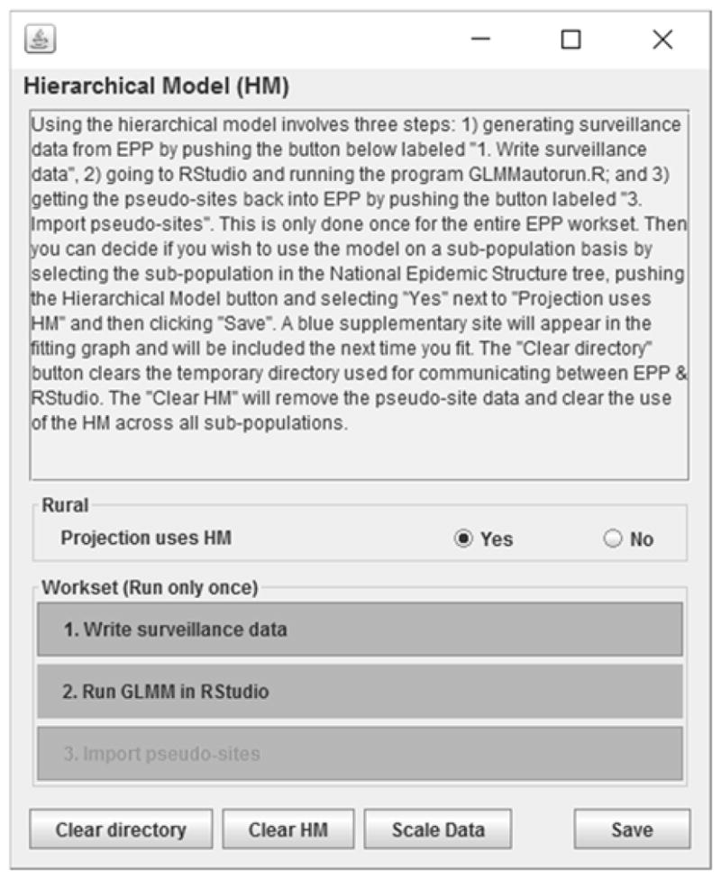
The Hierarchical Model panel in EPP. Here the user conducts the simple steps needed to generate pseudo-sites for use in the fitting (numbered buttons at the bottom) and determines if the currently selected projection is to use the pseudo-site in its fitting (“Projection uses HM” radio buttons).

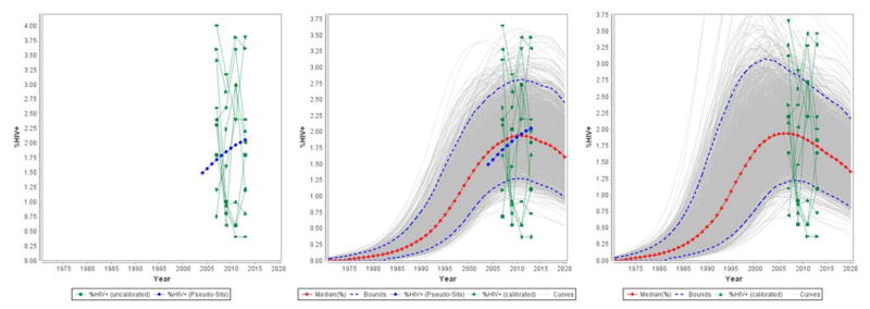
One writes the surveillance data, runs the hierarchical model on that surveillance data in RStudio, and then clicks on “Import pseudo-sites” to make the pseudo-sites available to any projection where the user chooses to use it for fitting. If a projection is to use the hierarchical model, the pseudo-site’s data will appear as a blue colored site in the graph on the EPP Project Page, as shown in Figure 4. The user only needs to run fit in EPP now to incorporate the hierarchical model effects into the fitting.

Figure 4.

An example of the pseudo-site (blue site in the graph on the left) in an area with relatively little data, and the effect of fitting with (center) and without (right) the pseudo-site active. Note how the pseudo-site draws the fit to a slower initial rise and a later peak.

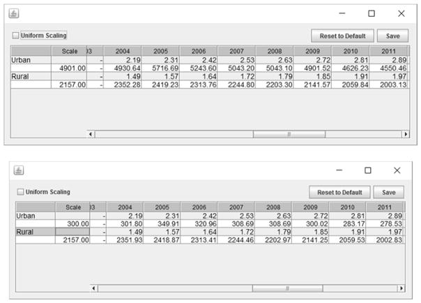
The amount of influence that the pseudo-site will have on the fit is determined by the sample sizes. In EPP those can be altered by clicking on the “scale data” button on the Hierarchical Model panel. This will bring up the scaling dialogue shown in Figure 5. By simply typing the desired average sample size into the “Scale” column, the user can alter the sample sizes of the data points from the pseudo-site. Larger sample sizes will increase the influence of the pseudo-site on the fitting.

Figure 5.

The scaling panel activated by the “Scale Data” button on the Hierarchical Model panel. By altering the value in the scale column, one changes the average sample size for the years where there are pseudo-site data. In this example, the top figure shows the default sample size of 4901 on average for the urban projection, while the lower figure shows the effect of changing this sample size to 300.

3. Results

In this section, we present an empirical study of the proposed model. We first describe the data we use and how we split the data into training and test sets. Then we discuss the selection of GLMM. After that we evaluate the performance of Spectrum/EPP with and without using auxiliary data. Finally, we show the fitted curves of the data.

3.1. Data description

We select the following four countries to demonstrate the empirical results of the proposed method: Liberia, Angola, Swaziland and Ghana. The data are provided by UNAIDS. Those four countries are selected as representatives of different data richness and prevalence level scenarios. Table 1 lists the data availability by years and number of sites for each of the four countries.

Table 1.

Summary of data availability of the selected four countries.

		Number of Clinics	Years of Data	Average Sample Size per Site	Population-based Survey
Angola	Urban	38	6	488	Not Available
	Rural	10	4	475
Liberia	Urban	22	7	405	2 years
	Rural	10	4	444
Ghana	Urban	23	22	427	2 years
	Rural	17	21	440
Swaziland	Hhohho	5	9	228	1 year
	Manzini	5	9	213
	Shiselweni	5	9	182
	Lubombo	6	9	202

In Angola and Liberia, compared to the urban sites the rural areas have fewer sites and insufficient years of data to indicate a clear trend in prevalence. In Liberia, the data is anchored by a survey, while Angola is not. In Ghana, all areas have relatively rich data and population survey data. In Swaziland, there are four areas of sparser data rather than just rural and urban, each of which has only 5 or 6 sites plus a single year of surveys. Moreover, Swaziland’s national prevalence level is above 20% while the other three countries are under or around 5%.

3.2. GLMM selection

We fit both the Binomial GLMM and Beta-Binomial GLMM within each country. The model is estimated using R INLA package [10]. The estimated over-dispersion parameters of the Beta-Binomial models are all close to zero, ranging from 0.00192 to 0.00902. For the Binomial model, we visually inspect the QQ plot of the standardized Pearson residuals versus the theoretical standardized Pearson residuals of the Binomial distribution, and find they line up very well along each other. Both the magnitude of the over-dispersion parameters in the Beta-Binomial models and the residual diagnostics of the Binomial models suggest that there is not much evidence of over-dispersion. Moreover, the Binomial model runs 2 to 20 times faster than the Beta-Binomial model. Therefore, we use the Binomial GLMMs to generate the area-specific prevalence estimates and create pseudo-sites.

3.3. Model Prediction Accuracy

We summarize the test data evaluation results in Table 2, with the minimum MAE and CPRS for each area highlighted in bold. We have the following observations:

Table 2.

Summary of mean absolute error (MAE) and continuous ranked probability score (CRPS) of the test set prediction with various average sample sizes for the pseudo site. All numbers are in percentages. The number of data years and the average number of sites of the training set are shown in parentheses. Sample size 0 corresponds to the case with no auxiliary data. The smallest MAE and CRPS of each area are in bold.

	Sample Size	MAE	CRPS	MAE	CRPS
Angola		Rural (1 year, 10 sites)		Urban (3 years, 25 sites)
	0	1.144	0.711	1.097	0.813
	4508 (GLMM)	1.058	0.677	1.099	0.814
	10	1.058	0.679	1.101	0.815
	100	1.067	0.682	1.094	0.811
	1000	1.047	0.675	1.101	0.813
		Rural (2 years, 4.5 sites)		Urban (5 years, 8 sites)
Liberia	0	2.866	2.228	1.559	1.033
	560 (GLMM)	2.379	1.919	1.589	1.053
	10	2.466	1.948	1.535	1.022
	100	2.418	1.931	1.547	1.025
	1000	2.377	1.915	1.561	1.037
		Rural (16 years, 7.9 sites)		Urban (17 years, 20.7 sites)
Ghana	0	0.753	0.507	0.925	0.647
	5653 (GLMM)	0.748	0.504	0.924	0.648
	10	0.741	0.499	0.928	0.650
	100	0.746	0.503	0.924	0.647
	1000	0.750	0.504	0.930	0.651
		Hhohho (6 years, 2 sites)		Manzini (6 years, 2 sites)
Swaziland	0	4.565	3.665	6.019	3.991
	1272 (GLMM)	4.452	3.530	6.157	4.100
	10	4.278	3.389	6.657	4.680
	100	4.420	3.483	6.427	4.392
	1000	4.451	3.530	6.273	4.202
		Shiselweni (6 years, 2 sites)		Lubombo (6 years, 2.2 sites)
	0	6.066	4.812	4.851	3.555
	1272 (GLMM)	6.117	4.982	4.610	3.328
	10	6.151	5.076	4.490	3.179
	100	6.134	5.040	4.506	3.194
	1000	6.130	5.012	4.601	3.314

1. Out of the 10 areas in the 4 countries, 8 areas show improvements in out-of-sample prediction by adding auxiliary data regardless of the auxiliary sample size. The original EPP is preferred in 2 areas of Swaziland.

2. In the areas where auxiliary data improve the prediction, the optimum sample size varies.

3. The most improvement lies in the data sparse areas borrowing information from data rich areas, as in Angola Rural and Liberia Rural. The auxiliary data with sample size 1000 offers the minimum MAE and CRPS in both cases. The MAE is increased by 8.5% and 17.1% for Rural Angola and Rural Liberia, and the CRPS is increased by 5.1% and 14% for the two areas. The GLMM estimated sample size is the next best scenario and provides similar improvements.

4. In data rich areas, such as Urban Angola, Urban Liberia, and both areas in Ghana, we see marginal improvement using auxiliary data.

5. In Swaziland, each area has about only 2 sites. The effects of adding a pseudo-site is mixed. In two of the areas, adding a pseudo-site with a small sample size (10) shows significant improvement. In the other two areas, no auxiliary data is preferred. One possible explanation is that due to the small number of existing sites (2 per area), the results highly depend on whether the samples and trends in the 8 sites are similar, since changing the number of sites from 2 to 3 can have a large impact on estimating the site effects.

6. Finally, we observe that higher prediction error is related to higher prevalence rates, as seen in the comparison between Swaziland and the other 3 countries.

Based on the above findings, we believe adding auxiliary data has benefits in most situations and recommend the GLMM estimated sample size as the default setting.

3.4. Data results

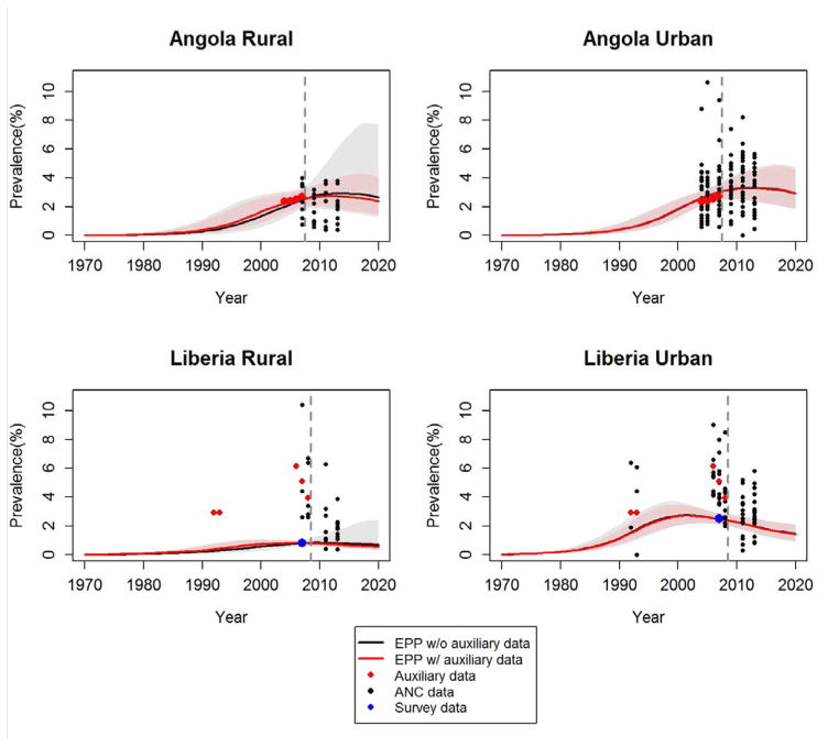
We compare the entire prevalence trajectories of the EPP fits between no auxiliary data and using auxiliary data with GLMM estimated size. For Ghana and Swaziland, the national prevalence trends look the same. Therefore, in Figure 6, we only present the national prevalence estimates for Angola and Liberia. We notice that the national trends and uncertainties with (red) and without (black) auxiliary data are similar in urban areas. Using auxiliary data provides much narrower uncertainty bounds than not using auxiliary data in rural areas. Moreover, with auxiliary data, the projected trend stabilizes from 2008 to 2010 in Rural Angola, and slightly declines in Rural Liberia after 2010. Both trends are more consistent with the observed data when the auxiliary data trends are included.

Figure 6.

The EPP model fitted to sub-national datasets from Angola and Liberia. The black curves and grey shaded areas show the posterior median and 95% uncertainty bounds estimated without using auxiliary data; the red curves and pink shaded areas show the posterior median and 95% uncertainty bounds estimated using auxiliary data with the GLMM estimated sample size; the black dots are the antenatal clinic prevalence; the blue dot is the survey prevalence; the red dots are the auxiliary data.

4 Discussion

In this paper, we apply the methodology in Bao et. al. [4] to four countries with different data availability. We discuss in detail the implementation of the method and its interface in Spectrum/EPP. We examine the effects of different auxiliary data sample sizes on the model’s prediction accuracy using several measures. The empirical results suggest that, for areas with sparse data and existence of relatively richer data in other areas, adding auxiliary data could improve the EPP fit. We allow EPP users to specify the auxiliary data sample sizes, and recommend using the default sample size provided by GLMM. Though we use the Binomial GLMM as the prior model in our empirical study, we propose the Beta-Binomial GLMM that accounts for sample correlations within a clinic as an alternative.

We find the most improvement lies in Angola and Liberia, where data are sparse in the rural areas and richer in the urban areas. As countries move to sub-national estimations, this pattern of sparsity is particularly true in settings where some regions had surveillance introduced early on and have long time trends, but numerous other regions have only been added to the surveillance system in recent years. The ability of the hierarchical model approaches described here to share data from the data-rich regions with longer time trends can lead to more realistic fits sub-nationally and, thus, improve aggregated national estimates.

In countries where all areas have limited data, especially small numbers of sites, we do not recommend using the auxiliary data. In those settings, the EPP trends can be highly affected by adding the auxiliary data and the outcomes are not guaranteed.

One potential further improvement for rich data situation is to add social, economic, and environmental factors as covariates in the hierarchical model. For countries without data rich areas, we would consider applying the hierarchical model to multiple neighboring countries so that information can be borrowed across countries. Although careful consideration would be needed to take into account the potential similarities and differences in the epidemics among the countries before applying such a model.

While beyond the scope of this paper, the same approach can be extended to model multiple high-risk groups in a country. The combination of a sub-national region and a particular high-risk group can have sparse data. In the GLMM, we have one more layer of data structure that makes the observation y_agit, where g is the high-risk group indicator. We can simply treat the groups the same way as we treat areas, and introduce group-specific intercept and time trends. We will then generate area and group specific pseudo-sites. Any general sub-epidemic can be estimated in a similar manner.

References

- 1.UNAIDS. Global AIDS update. 2016 http://www.unaids.org/en/resources/documents/2016/Global-AIDS-update-2016.
- 2.Brown T, Bao L, Eaton JW, Hogan DR, Mahy M, Marsh K, Mathers BM, Puckett R. Improvements in prevalence trend fitting and incidence estimation in EPP 2013. AIDS. 2014;28(Suppl 4):415–426. doi: 10.1097/QAD.0000000000000454. [DOI] [PMC free article] [PubMed] [Google Scholar]
- 3.Ghys PD, Brown T, Grassly NC, Garnett G, Stanecki KA, Stover J, Walker N. The UNAIDS estimation and projection package: A software package to estimate and project national HIV epidemics. Sexual Transmitted Infections. 2004;80(Suppl 1):5–9. doi: 10.1136/sti.2004.010199. [DOI] [PMC free article] [PubMed] [Google Scholar]
- 4.Bao L, Sheng B, Niu X, Tang Y, Brown T, Ghys PD, Eaton JW. Incorporating Hierarchical Structure into Dynamic Systems: an Application of Estimating HIV Epidemics at Sub-National and Sub-Population Level. 2016 https://arxiv.org/abs/1602.05665.
- 5.Spiegelhalter DJ, Best NG, Carlin BP, Van Der Linde A. The deviance information criterion: 12 years on. Journal of the Royal Statistical Society: Series B. 2014;76(3):485–493. [Google Scholar]
- 6.Spiegelhalter DJ, Best NG, Carlin BP, Van Der Linde A. Bayesian measures of model complexity and fit. Journal of the Royal Statistical Society: Series B. 2002;64(4):583–639. [Google Scholar]
- 7.Stover J, Brown T, Marston M. Updates to the Spectrum/Estimation and Projection Package (EPP) model to estimate HIV trends for adults and children. Sexually Transmitted Infections. 2012;88(Suppl 2):11–16. doi: 10.1136/sextrans-2012-050640. [DOI] [PMC free article] [PubMed] [Google Scholar]
- 8.Bao L. A new infectious disease model for estimating and projecting HIV/AIDS epidemics. Sexually Transmitted Infections. 2012;88(Suppl 1):58–64. doi: 10.1136/sextrans-2012-050689. [DOI] [PMC free article] [PubMed] [Google Scholar]
- 9.Alkema L, Raftery AE, Clark SJ. Probabilistic projections of HIV prevalence using Bayesian melding. Annals of Applied Statistics. 2007;1:229–248. [Google Scholar]
- 10.Rue H, Martino S, Chopin N. Approximate Bayesian inference for latent Gaussian models using integrated nested Laplace approximations (with discussion) Journal of the Royal Statistical Society, Series B. 2009;71(2):319–392. [Google Scholar]
- 11.Gneiting T, Raftery AE. Strictly Proper Scoring Rules, Prediction, and Estimation. Journal of the American Statistical Association. 2007;102(477):359–378. [Google Scholar]