Co-occurrence of extremes in surface ozone, particulate matter, and temperature over eastern North America

Significance

Exposure to extreme temperatures and high levels of the pollutants ozone and particulate matter poses a major threat to human health. Heat waves and pollution episodes share common underlying meteorological drivers and thus often coincide, which can synergistically worsen their health impacts beyond the sum of their individual effects. Furthermore, there is evidence that pollution episodes and heat waves will worsen under future climate change, making it imperative to understand the nature of their co-occurrence. In this paper, using 15 years of surface observations over the eastern United States and Canada, we show that the extremes cluster together in often overlapping large-scale episodes, and that the largest episodes have the hottest temperatures and highest levels of pollution.

Abstract

Heat waves and air pollution episodes pose a serious threat to human health and may worsen under future climate change. In this paper, we use 15 years (1999–2013) of commensurately gridded (1° x 1°) surface observations of extended summer (April–September) surface ozone (O₃), fine particulate matter (PM_2.5), and maximum temperature (TX) over the eastern United States and Canada to construct a climatology of the coincidence, overlap, and lag in space and time of their extremes. Extremes of each quantity are defined climatologically at each grid cell as the 50 d with the highest values in three 5-y windows (∼95th percentile). Any two extremes occur on the same day in the same grid cell more than 50% of the time in the northeastern United States, but on a domain average, co-occurrence is approximately 30%. Although not exactly co-occurring, many of these extremes show connectedness with consistent offsets in space and in time, which often defy traditional mechanistic explanations. All three extremes occur primarily in large-scale, multiday, spatially connected episodes with scales of >1,000 km and clearly coincide with large-scale meteorological features. The largest, longest-lived episodes have the highest incidence of co-occurrence and contain extreme values well above their local 95th percentile threshold, by +7 ppb for O₃, +6 µg m⁻³ for PM_2.5, and +1.7 °C for TX. Our results demonstrate the need to evaluate these extremes as synergistic costressors to accurately quantify their impacts on human health.

Statistically extreme events in pollution and weather often pose risks to human health. In this paper, using 15 y of observations over eastern North America (ENA), we examine three health extremes: surface ozone (O₃), fine particulate matter (PM_2.5, defined as aerosols of diameter ≤2.5 µm), and heat waves, measured as maximum temperature (TX). O₃ and PM are the two major air pollutants threatening human health (1). Heat waves also pose a major threat to human life (2–4). The average magnitude of local air pollution is controlled primarily by local and regional emissions of the pollutants and their precursors, but, like heat waves (5), extreme air pollution is often driven by synoptic meteorology (6, 7). These three extremes are often associated with slow-moving high-pressure systems that accumulate pollutants and heat owing to the overlying meteorological conditions, namely high temperatures, abundant solar insolation, low precipitation, and low wind speeds (7–10).

Aside from the direct influence of meteorology, there exist multiple interactions and feedbacks that act further to exacerbate extreme conditions. For example, the high temperatures during a heat wave increase emission rates of biogenic volatile organic compounds, which augment the production of surface O₃ and secondary organic aerosols (i.e., PM_2.5). The drought-like conditions that often accompany heat waves can inhibit stomatal uptake of O₃ (11) and, through soil moisture feedback, can both amplify the heat waves and worsen air quality (12). Energy demands for air-conditioning increase during heat waves (13), which increases anthropogenic emissions and thus pollutant abundance. In any case, the extremes often co-occur as a result of their shared underlying drivers, greatly increasing the risks to human health (14). The imperative to understand the co-occurrence of health extremes is driven in part by the recognition that episodes of extreme temperatures (15–18) and poor air quality (19–24) may become more frequent, longer lasting, and more intense in a warming climate, in which many climate-driven feedbacks can alter air quality independent of emissions (e.g., 8, 10, 25, 26).

That combined extremes produce greater impacts or risks than those summed simply from single extremes acting alone is a prevalent concept in the climate change community (27). In this case, however, the multiple stressors go beyond physical extremes—such as the health events analyzed here—to include economic, social, and political events (figure 1.5 in ref. 28). There is evidence indicating that combined pollution extremes and heat waves are such synergistic stressors (i.e., impact modifiers), and that combined extremes produce disproportionately greater adverse health impacts (14, 29–33).

Here we used the methods developed in previous work (24, 34, 35) to calculate regularly gridded, daily surface values for O₃, PM_2.5, and temperature. These quantities are continuous with real units (parts per billion by molar fraction, micrograms per cubic meter, and degrees Celsius), which allowed us to develop a probability distribution for each grid cell and define extreme events in terms of a return time or frequency (days per year). An important, relevant finding from previous work was that the O₃ levels in an extreme pollution episode generally increase with increasing geographic extent and duration of the episode (35).

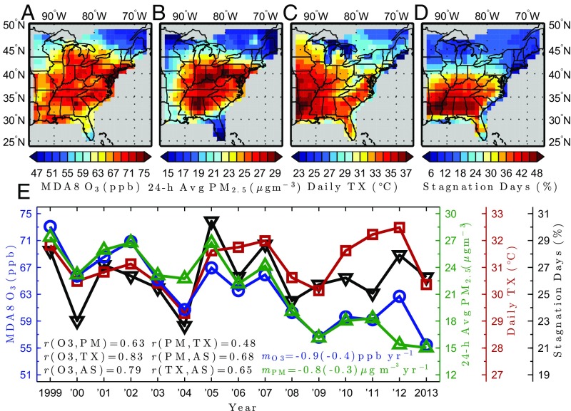
The use of a daily air stagnation index (ASI) (36) as a proxy for health extremes has been developed further by others (26, 37), and we include the ASI here because stagnation describes the basic meteorological conditions that exacerbate pollution episodes and heat waves. However, this index is Boolean and thus cannot be used to define extreme events in terms of frequency or magnitude; for example, approximately 40% of summer days are considered stagnant in the southeastern United States, compared with approximately 20% in the more polluted northeastern states (Fig. 1D).

Fig. 1.

Spatial patterns and time series of extreme thresholds. (A–C) 95th percentile of April–September 1999–2013. (A) MDA8 O₃ (ppb). (B) 24-h average PM_2.5 (μg m⁻³). (C) daily maximum temperature (°C). (D) Air stagnation frequency (% of days). (E) Annually derived 95th percentile of the quantities in A–D, indicated by blue, green, red, and black lines, respectively. Also shown are linear trends of 95th percentile (median) MDA8 O₃ (ppb yr⁻¹) and 24-h average PM_2.5 (μg m⁻³ yr⁻¹), along with interpair correlations of all quantities (MDA8 O₃ and 24-h average PM_2.5 trends removed).

We begin by defining extreme events, taking into account the nonstationarity of all three extremes. We then present a case study of an episode of co-occurring extremes and build a climatology of the statistics of overlap and lag in space and time. We conclude by attempting to understand the unique spatiotemporal patterns found for each of our health extremes. Overall, the clear identification of large, overlapping extreme pollution episodes—quantified in terms of observations of O₃, PM_2.5, and temperature—provides a baseline evaluation for any model used to project future air quality and heat waves.

Results

Defining Extreme Events and Episodes.

Previous work (24, 34, 35) has defined O₃ extremes over the 2000–2009 decade in a local climatological manner as the 100 d (∼97.3th percentile) with the highest maximum daily 8-h average (MDA8). This approach enabled clear identification of large-scale multiday pollution episodes consisting of connected, locally extreme daily events that were not readily seen using the US Environmental Protection Agency’s (EPA) absolute threshold approach. That is, neighboring regions often have large systematic differences in absolute O₃ levels, and thus a 75-ppb exceedance in one cell might not occur in its neighboring cell even though both had a 97th percentile event. Here we continue this approach (i.e., number of events = 10 times the number of years) to define extremes in O₃, PM_2.5, and daily TX. These three quantities can be treated identically, using their local probability distributions to define extreme events; however, the ASI, being Boolean, cannot define extremes in terms of severity.

PM_2.5 extremes can occur in both summer and winter in ENA (38), but because the vast majority of temperature and O₃ extremes occur between late spring and early fall, our statistics consider only days during the extended summer season (April 1– September 30). We adopt the ∼95th percentile (see below) as the local extreme threshold, because that is equivalent to our 100-d per decade definition if all extremes occur during this extended summer period. Alternative heat wave definitions exist (39), but our choice maintains consistency across all three quantities and is remarkably close to the local 95th percentile warm season (May 1–September 30) temperature used by Anderson and Bell (39). Their definition, unlike ours, requires two consecutive exceedance days, but most of our extremes are multiday.

Fig. 1 A–C shows the 95th percentile over the entire period (1999–2013) for the three observed extremes at each grid cell. The 95th percentile of MDA8 O₃ (Fig. 1A) has an approximate range of 45–80 ppb across the domain, with the highest abundances in the Ohio River Valley and along the eastern urban corridor. The 95th percentile of PM_2.5 (Fig. 1B) ranges from approximately 15 to 30 μg m⁻³, with a swath of >25 μg m⁻³ almost everywhere east of the Mississippi River between 33°N and 43°N. The 95th percentile of TX (Fig. 1C) is highest in the southwest sector of the domain (>37 °C) and decreases monotonically to its minimum over the Great Lakes and the northeast sector (<23 °C). Fig. 1D shows stagnation day frequency, which accounts for >30% of the extended summer days in almost all grid cells south of 40°N and >40% in a swath across the Gulf Coast states. Stagnation is much less common in the north and drops dramatically northward across 40°N. Averaged over our domain, ∼26% of the days are stagnant, many more than the upper 5% used for our extreme criteria.

Trends in Air Quality and Temperature.

Precursor emission reductions resulted in a clear decreasing trend in the 2000–2009 gridded MDA8 O₃ time series of Schnell et al. (34), causing the identification of more extremes in the early part of the decade. Emission reductions have been similarly effective in reducing PM_2.5. Fig. 1E shows the domain-averaged annual value of the quantities shown in Fig. 1 A–D. Air quality management has reduced the highest values of both MDA8 O₃ and 24-h average PM_2.5, with annual 95th percentile trends from 1999 to 2013 of –0.9 ppb y⁻¹ for O₃ and –0.9 μg m⁻³ y⁻¹ for PM_2.5 (P < 0.01 for both). These reductions are much greater than those in the median, with trends for O₃ and PM_2.5 of –0.4 ppb y⁻¹ and –0.3 μg m⁻³ y⁻¹, respectively (P < 0.01 for both). Temperature extremes are also occurring on an overall warming background (40), but the 95th percentile trend here is not significant at the 95% confidence level. Stagnation frequency has no obvious trend, but the interannual variability (IAV) follows the other three quantities (see the correlations, r, in Fig. 1E). These trends must be accounted for when identifying extreme events. One solution is to force each year to have the same number of events (10), but then IAV information is lost. Indeed, the 95th percentile values of O₃ and PM_2.5 when calculated annually show very similar IAV values, with a correlation coefficient of 0.63 over their detrended 1999–2013 time series (Fig. 1E). Some factors, such as wildfires, may drive IAV in PM_2.5 (8), but not necessarily O₃. The magnitude of the interpair correlations shown in Fig. 1E, especially those with stagnation, indicates that meteorology is the most likely factor driving the extremes (41, 42). To minimize contamination by background trends while preserving interannual meteorological variability, we break the 1999–2013 O₃ and PM_2.5 time series into three 5-y windows. To avoid similar bias in temperature, we treat the temperature record similarly. We follow the methods of Schnell et al. (34) and define extreme events in MDA8 O₃ (O3X), 24-h average PM_2.5 (PMX), and daily maximum temperature (TXX) at each grid cell as the 50 d with the highest values in each 5-y window (∼94.5th percentile).

An Example of Co-Occurrences: June 20–28, 2005.

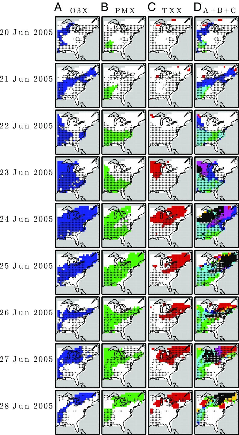
Fig. 2 A–D shows columns of a daily sequence (rows) of extreme maps for the multiday pollution episode of June 20–28, 2005. The first three columns (Fig. 2 A–C) show O3X (blue), PMX (green), and TXX (red). The fourth column (Fig. 2D) shows a combination of the first three columns, identifying cells with single or co-occurring extremes. For a single occurrence, the cell retains the same color as in first three columns, whereas cells with co-occurrences are colored with the combined colors. Stippling denotes a grid cell stagnation day. Animations showing maps of the identified extremes, co-occurrences, and stagnation for each day of the 15-y record (separated into three 5-y movies) are provided in Movies S1–S3.

Fig. 2.

Nine-day (June 20–28, 2005) episode progression for O3X (blue) (A), PMX (green) (B), TXX (red) (C), and their combinations (D). Colors in D correspond to the combined individual RGB triplets, i.e., O3X+PMX (cyan), O3X+TXX (magenta), PMX+TXX (yellow), and O3X+PMX+TXX (black). Stippling denotes an identified stagnation day (white stipples in D if the grid cell has all three extreme types).

The episode began on June 20 (Fig. 2, top row) on the western edge of the domain with O3X and PMX. The episode grew in size and propagated eastward over the next 3 d. O3X first extended in a thin southwest-northeast filament along the leading edge of a cold front, then eventually covered most of the domain by June 24. (Weather map access is discussed in Materials and Methods.) PMX coverage first extended eastward, and then built over the upper midwest along the western edge of the surface high on June 23. This feature highlights the potential role of meteorological transport on the location and timing of PMX. For example, because the highest PM_2.5 abundances are found in the southeast (both in this example and on average; Fig. 1B), anticyclonic circulation can transport high-PM_2.5 air to relatively cleaner areas, such as the upper midwest. Indeed, PM_2.5 extremes in the United States have been found to occur on the backside of high-pressure systems (43). TXX were rare until June 23, when they then occurred in the northwest quadrant of the domain behind a warm front. Over the entire 9-d sequence, TXX occurred almost exclusively in the northern half of the domain. By June 24, the high-pressure ridge enveloped most of the domain, and the episode reached its maximum size; 87% of the grid cells had at least one type of extreme, 64% had at least two types, and 23% had all three types. Over the final 3 d, the episode moved eastward and decreased in size, likely owing to widespread precipitation over the region. The identified ASI days show erratic overlap with the health extremes, sometimes coinciding almost exactly (PMX on June 22) and sometimes being exclusive (TXX on June 23–24). However, the rows of Fig. 2D show that in most cases, at least one type of extreme occurred when the grid cell was considered stagnant (68% of all grid cells and days).

Although the foregoing example is one of the larger episodes, it is hardly unusual (Discussion and Movies S1–S3), and we find that stagnation and most extreme levels of O₃, PM_2.5, and TX occur in large-scale, multiday, coherent structures. The individual extremes also tend to group together within their own smaller-scale clusters but often overlap (i.e., co-occurrences).

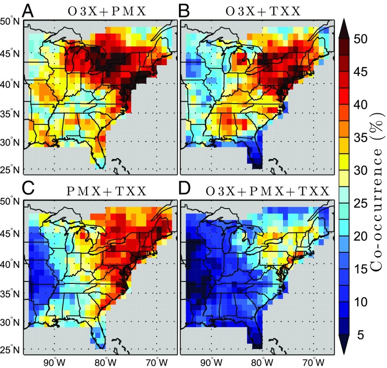
Fig. 3 shows the frequency of co-occurrence over the entire 15-y period (percentage of 150 events) at each grid cell for the three two-event combinations (i.e., O3X+PMX, O3X+TXX, and PMX+TXX in Fig. 3 A–C, respectively) and the three-event combination (Fig. 3D). Averaged over the domain, O3X+PMX was most likely (35%), followed by O3X+TXX (30%), PMX+TXX (29%), and O3X+PMX+TXX (16%). The greatest co-occurrence frequencies for all event combinations are seen in the northeast, >50% for any two co-occurring events and ∼30% for all three. The lowest co-occurrence frequencies are found in Florida, the Gulf Coast, and the western edge of the domain (44). The generally lower (higher) co-occurrences in the southwest (northeast) imply that the extremes are caused by different (similar) synoptic drivers. In the north, the extremes may be related to cold front frequency (and thus high-pressure persistence), whereas the low values in the south may be caused by opposing effects of the Bermuda High (45).

Fig. 3.

Co-occurrence frequency (% of 150 events) for O3X+PMX (A), O3X+TXX (B), PMX+TXX (C), and O3X+PMX+TXX (D).

The extremes may show consistent offsets in space and time owing to set spatial patterns in precursor emissions or meteorology and related transport. For example, temperature is a well-known driver of O₃ production (46), and thus TXX may precede O3X in grid cells with large precursor emissions (7, 47). Owing to the typical eastward progression of weather systems, this mechanism may result in displacement of O3X westward of TXX.

Systematic Offsets in Space.

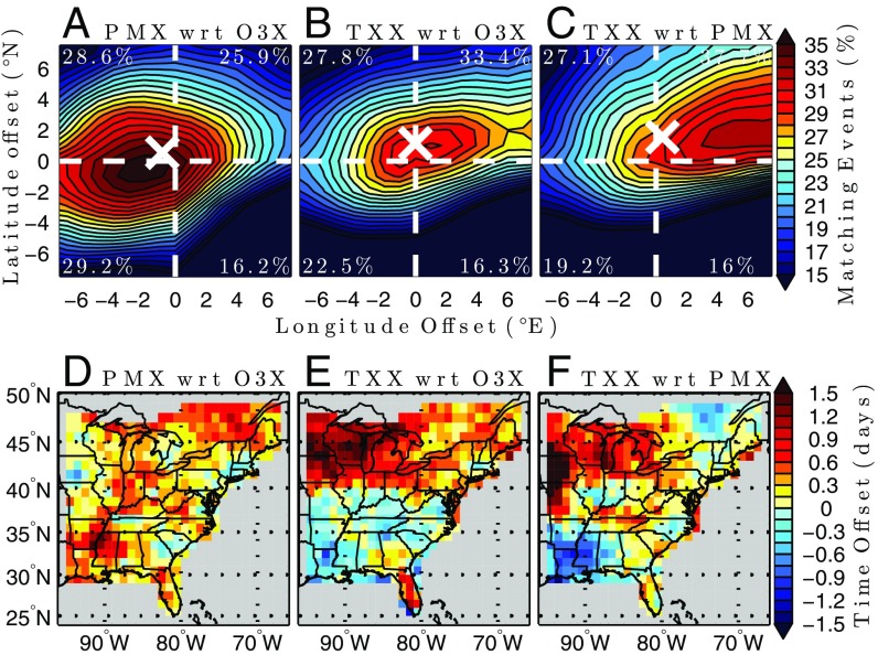
We tested for systematic spatial offsets by calculating co-occurrence frequency as a function of spatial lag averaged across all grid cells. The 1° × 1° domain extended 27° in latitude and 30° in longitude, but because the extremes are unlikely to be correlated beyond ∼500–1,000 km, we limited the lags to ±8° and did not extrapolate any grid cell’s lags beyond the masked domain. Fig. 4 A–C shows the domain average co-occurrence as a function of spatial lag for the corresponding co-occurrence types in Fig. 3 A–C. Also provided is the fraction in each quadrant and the 2D weighted centroid (white X). Note that the (0°, 0°) lag represents the domain average co-occurrences in Fig. 3 A–C. The notation is as follows: for PMX with respect to O3X (Fig. 4A), the contours show the likelihood (% of events) that PMX occur at the latitude-by-longitude offset in 1° cells from O3X. For example, Fig. 4A shows that the highest coincidence of PMX+O3X (35%) is roughly centered on (latitude, longitude) = (0°, 0°), but that on average, PMX occur to the northwest of O3X (+0.5°, –0.8°) and at a maximum to the southwest. The relatively large region of high values in Fig. 4A shows that O3X and PMX co-occur not only more frequently, but also over larger spatial scales than either do with TXX. TXX tend to occur to the northeast of both O3X (+1.1°, +0.01°) and PMX (+1.6°, +0.4°). These offsets are averaged over the full domain for more robust statistics; however, it is clear that patterns vary across the domain (see below), and that conclusions based on the domain average might not apply in all regions. These spatial offsets can be manifestations of offsets in time, because large episodes typically propagate eastward across the domain. For example, the westward displacement of PMX with respect to O3X (Fig. 4A) may be evidence that PMX occur after O3X at a given grid cell (i.e., after the O3X episode has moved east).

Fig. 4.

Spatial and temporal offsets of co-occurrences. (A–C) Domain average co-occurrence (%) as a function of spatial lag (degrees) for PMX with respect to O3X (A), TXX with respect to O3X (B), and TXX with respect to PMX (C). Also shown are the 2D weighted centroids (white Xs) and the average value of each quadrant. (D–F) Weighted average temporal lag (days) at each grid cell for the corresponding event co-occurrence types in A–C.

Systematic Offsets in Time.

We tested for systematic temporal offsets by calculating the frequency of co-occurrence at each grid cell as a function of time lag, from –7 to +7 d. Fig. 4 D–F shows the weighted average lag (in days, with weights equal to each lag’s co-occurrence frequency) at each grid cell for the corresponding event co-occurrence types in Fig. 3 A–C. For example, Fig. 4D (PMX with respect to O3X) shows positive values (∼1 d) over much of the domain, meaning that PMX occur approximately 1 d after O3X. We can speculate on the mechanisms for this lag, but an understanding will require a well-tested model that reproduces these observations. For example, the PMX delay may occur simply because PM_2.5 simply takes longer to accumulate than O₃, or because the different diurnal cycles and averaging windows cause a shift in PM_2.5 to the next morning. The TXX with respect to O3X map (Fig. 4E) shows a sharp regime shift at 40°N. To the north of 40°N, TXX occur 1–2 d after O3X; but to the south, TXX precede O3X by ∼1 d (except in parts of Florida and Georgia). The south shows the expected temperature–O₃ causal relationship in which O₃ abundance increases following a temperature increase. To the north, we may be seeing quicker activated photochemistry with respect to temperature or evidence of suppression of O₃ by high temperatures. This suppression has been identified previously, with one study implicating enhanced PAN decomposition and reduced isoprene emissions (48), and another study finding that the suppression is caused not by temperature-dependent effects on chemistry or emissions, but rather by a breakdown in the linearity of meteorology–O₃ correlations (44). In any case, it is not clear why this relationship changes at 40°N. The TXX with respect to PMX map (Fig. 4F) is essentially Fig. 4E minus Fig. 4D. TXX typically occur after PMX, except in the southwest corner of the domain and parts of Canada.

Average Progression of Large Episodes.

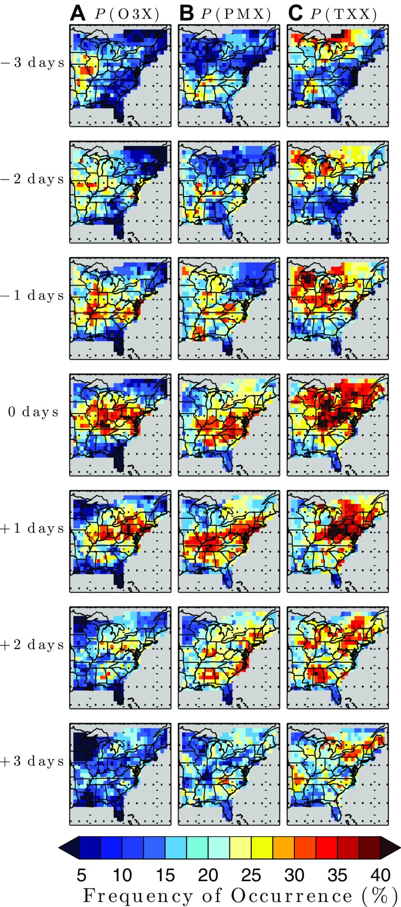
The systematic spatial and temporal offsets among the three different extremes suggests that there may be a typical evolution of a multiextreme episode, such as which extremes appear first and where. Based on a daily composite of all large, weeklong episodes (Fig. S1 and SI Text), we can describe the evolution of these “superepisodes.” At the start, O3X were most likely in the area west of 90°W from 35°N–45°N, PMX dominated south of 40°N, and TXX were most common north of 40°N, except in New England. Over the next 3 d, the frequencies increased for all three extremes, with the highest values moving generally eastward. For the central episode day, O3X occurred with greatest frequency (>30%) in a band at 35°N–45°N across the domain, PMX occurred with greatest frequency in a band at 32°N–41°N, and TXX occupied the top half of the domain (36°N–48°N) and were most common overall (>40% in some grid cells). O3X disappeared the most rapidly, whereas TXX remained frequent in the northeast. The average pattern shown in Fig. S1 resembles the pattern seen in June 22–28 of the sample episode in Fig. 2.

Fig. S1.

Progression of average large-scale episodes, shown as the frequency (%) of events in each grid cell over 30 weeklong episodes in 15 y. The rows show the 7-d sequence about the central day. Columns from left-to-right show the fraction for O3X (A), PMX (B), and TXX (C). If events were random with respect to the episodes, then the fraction would be 5%.

Whether these observed patterns can provide a semiempirical prediction capability is not clear; nevertheless, they do provide stringent observational tests for models used in air quality predictions. Most notably, the size of heat waves is clearly larger (in space and time) than either pollution extreme. This difference is likely emissions-driven, because pollution precursors, although ubiquitous over ENA, are not as uniform as the meteorology.

Size and Enhancement of Extreme Episodes.

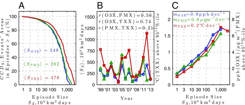
The clustering algorithm (Materials and Methods) identifies connected-cell, multiday episodes of size S (units = 10⁴ km² d = ∼1° grid cell). Fig. 5A shows the distribution of episode sizes for each type of extreme as the complementary cumulative distribution (CCD), i.e., the fraction of events’ time integrated area occurring in episodes of size S or larger (see figure 11 of ref. 34). Fig. 5A can be read as saying that ∼100% of all events occur in episodes with S >1 × 10⁴ km² d (by definition), 90% occur with S >30 × 10⁴ km² d, and that 40% of O3X and PMX events occur in episodes of size S >500 × 10⁴ km² d. The TXX episodes are larger, and the larger episodes contain a greater fraction of the events; 40% occur in episodes of size S >900 × 10⁴ km² d. Average episode sizes,〈S〉, calculated as a geometric mean with weights equal to S, confirm that TXX episodes are clearly larger:〈S_TXX〉= 478 × 10⁴ km² d;〈S_O3X〉= 249× 10⁴ km² d; and〈S_PMX〉= 282 × 10⁴ km² d. The annual variation in〈S〉(Fig. 5B) shows moderate correlation across the three extremes, with paired correlation coefficients ranging from 0.21 to 0.74. O3X and TXX are the most closely correlated, but TXX clearly shows years with large heat waves that are not matched in PMX and O3X (i.e., 1999, 2006, 2007, and 2012).

Fig. 5.

Episode sizes and enhancements. (A) CCD (%) of the total areal extent of extreme events as a function of episode size S (10⁴ km² days) for O3X (blue), PMX (green), and TXX (red) episodes. Average episode sizes 〈S〉 over the 15-y period are provided in the inset. (B) Annual derived average episode size 〈S〉 for each extreme type and paired correlation coefficients (r). (C) Average value of the extreme events (ppb for O3X, µg m⁻³ for PMX, °C for TXX) relative to the 95th percentile as a function of episode size. Also shown is the slope of the enhancement per log-decade in S.

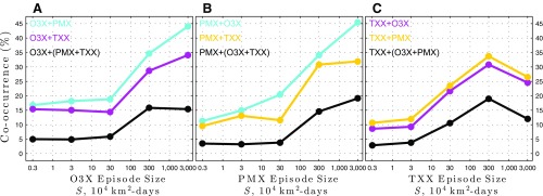
Co-occurring extremes at a cell-by-cell level are generally more likely for larger episodes and on days with maximum spatial coverage (Fig. S2), except for the largest TXX episodes (S >300 × 10⁴ km² d) where co-occurrence frequency decreases and likely reflects the propensity of TXX episodes to be significantly larger than O3X and PMX.

Fig. S2.

Co-occurrence frequency (%) as a function of episode size (S; 10⁴ km² d) for O3X (A), PMX (B), and TXX (C) episodes.

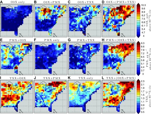
Identifying the size of an episode is highly valuable in terms of predictive capability of its severity. Using the 95th percentile as the baseline in each cell, we find a clear relationship between episode size and the value of the extremes above this baseline that is linear in log(S) (Fig. 5C). For episodes with S = 1,000 × 10⁴ km² d compared with those with S = 1 × 10⁴ km² d, O₃ abundances are 7 ppb higher, PM_2.5 abundances are ∼6 µg m⁻³ higher, and TX is ∼1.7 °C higher. Consistently across all episode sizes, the larger episodes have the highest pollution levels and the hottest temperatures. Each extreme is also greatest on average when it co-occurs with one or both of the other extremes and lowest when it occurs by itself (Fig. S3). This effect is most pronounced for the combination of all three extremes in the far northeast, with enhancements above the 95th percentile threshold of up to +10 ppb for O3X, +9 µg m⁻³ for PMX, and +2 °C for TXX.

Fig. S3.

Average values of O3X (ppb) (A–D), PMX (µg m⁻³) (E–H), and TXX (°C) (I–L) above the 95th percentile when occurring by themselves (A, F, K) and when they co-occur with one (B–C, E, G, I–J) or both (D, H, L) other extreme types.

Discussion

By combining detailed site measurements of surface O₃ and PM_2.5 over the ENA with meteorological reanalysis of surface temperatures, we have created a consistently mapped climatology of two different types of air pollution and heat waves on a standard 1° × 1° grid. The gridded results represent averaged quantities and thus are directly comparable to Earth system models. We present a wide range of statistics describing the space-time structure of the extremes, including their coincidence, spatial and temporal offsets with respect to one another, and overall large-scale connectedness and how it relates to their severity. This 15-y climatology is intended for the analysis of the structure and co-occurrence of extreme air pollution episodes and heat waves, impact studies on human health and agriculture, and chemistry-climate model evaluation. Thus, all datasets are objectively interpolated in space to give average values over each grid cell (34).

Extreme events tend to cluster into multiday, spatially connected episodes with spatial scales on the order 1,000 km or greater. For the largest episodes, values for O₃, PM_2.5, and temperature are well above the statistical threshold defining their extremes. Meteorology clearly drives the extremes, with the three different types of extreme episodes often coinciding or appearing slightly offset in space or time. The sequencing of events does not always support simple mechanistic arguments; for example, warmer temperatures make O₃ pollution more severe, because the O₃ events precede temperature events for much of the ENA. Obviously, there are many mechanisms driving these patterns of extremes of air pollution and temperature, and thus these observations present evidence of a model evaluation of cause.

Large-scale, overlapping extreme episodes pose the greatest potential health risk, not only because they coincide, but also because they are found to have the highest pollution levels and hottest temperatures. Thus, a multistressor approach must be taken when evaluating impacts on human health and vegetation. Furthermore, there is evidence that heat waves and pollution episodes will intensify under a warming climate in some regions, and thus we need to develop climate models that can effectively reproduce large-scale pollution episodes and heat waves.

Materials and Methods

We used a combination of surface monitoring station data and meteorological data over a 15-y period (1999–2013) to identify climatologically extreme events in each cell of a regular 1° × 1° grid over the ENA. For surface O₃, we used hourly abundances from the US EPA’s Air Quality System (AQS; https://www.epa.gov/aqs) and Clean Air Status and Trends Network (CASTNet; https://www.epa.gov/castnet) and Environment Canada’s National Air Pollution Surveillance Program (NAPS; maps-cartes.ec.gc.ca/rnspa-naps/data.aspx). The AQS and NAPS networks also provide observed daily average PM_2.5. The hourly O₃ and daily PM_2.5 abundances were interpolated onto a 1° × 1° grid over the ENA (96°W–66°W, 24°N–50°N) following the algorithm of Schnell et al. (34). MDA8 O₃ was derived at each grid cell from the interpolated hourly abundances. The disparity between the O₃ and PM_2.5 averaging windows reflects what is typically used for regulatory purposes and health impacts. For temperature, we used the European Centre for Medium-Range Weather Forecasting (ECMWF; apps.ecmwf.int/datasets/data/interim-full-daily/levtype=sfc/) reanalysis data, which provides gridded, 6-h maximum temperatures at a 2-m height. Daily maximum temperature was calculated as the maximum of each day’s four values. ECMWF data were taken from the available 0.5° × 0.5° grid, and four such cells were averaged to calculate our 1° × 1° product. As an additional analysis tool, we calculated the ASI following Horton et al. (37), using reanalysis data on 500-mb and 10-m wind speeds (2.5° remapped to 1°) from the National Centers for Environmental Prediction (www.esrl.noaa.gov/psd/data/gridded/data.ncep.reanalysis.html) and daily cumulative precipitation from the National Aeronautics and Space Administration’s Global Precipitation Climatology Project (49). A grid -cell day was considered stagnant at 10-m wind speed <3.2 m s⁻¹, 500-mb wind speed <13.0 m s⁻¹, and cumulative precipitation <1 mm. Daily weather maps referred to in the discussion of Fig. 2 can be obtained via the National Oceanic and Atmospheric Administration’s Weather Prediction Center (www.wpc.ncep.noaa.gov/dailywxmap/). The 1° × 1° datasets of MDA8 O₃, 24-h average PM_2.5, daily TX, and ASI are available from the corresponding author on request.

Large-scale, multiday pollution episodes were defined from the extreme events in each cell using a clustering algorithm (34). This method links events located within 1 d or 1° in latitude and longitude of one another, and thus episodes can be assigned a size (km² d) and followed throughout their synoptic development. We use “event” to describe a single-day statistical extreme at a cell and “episode” to describe a cluster of such events.

SI Text

The highest O₃ levels are associated with the largest episodes (35); thus, we limited our analysis to episodes (i.e., a connected set of any of the three extremes; Materials and Methods and ref. 34) that lasted at least 7 d and had at least 350 events of each type of extreme. These episodes were constructed by connecting grid cell days with any of the three extreme types (as opposed to connecting only extremes of the same type). We truncated these large-scale episodes to the central 7 d by defining the central day as the rounded value of the event-weighted average of the time indices and then limiting the episode to at most ±3 d from the central day. Visually, if all of the events (3 × 350) were within these 7 d, then the average spatial coverage of each extreme would be 50 grid cells (∼7° × 7°) with the largest coverage on the central day. Over the 15-y period, there were 30 such weeklong multi-extreme episodes, distributed roughly equally across the years (i.e., on average about 2 wk of each year, or 210 d total).

Fig. S1 shows the 7-d sequence in maps of the average large-scale episodes in O3X, PMX, and TXX. The seven rows show daily maps from 3 d before to 3 d after the central day of the episode. Each 1° cell in each daily map shows the fraction (%) of the 30 possible days that have an extreme event designated by the column. If the extreme events were random with respect to the large-scale episodes, then the frequency would be that of the events themselves, 5%, and we see such large random areas at the beginning and end of the 7 d for all three extremes.

References

- 1.Anenberg SC, Horowitz LW, Tong DQ, West JJ. An estimate of the global burden of anthropogenic ozone and fine particulate matter on premature human mortality using atmospheric modeling. Environ Health Perspect. 2010;118(9):1189–1195. doi: 10.1289/ehp.0901220. [DOI] [PMC free article] [PubMed] [Google Scholar]
- 2.Rooney C, McMichael AJ, Kovats RS, Coleman MP. Excess mortality in England and Wales, and in Greater London, during the 1995 heatwave. J Epidemiol Community Health. 1998;52(8):482–486. doi: 10.1136/jech.52.8.482. [DOI] [PMC free article] [PubMed] [Google Scholar]
- 3.Semenza JC, et al. Heat-related deaths during the July 1995 heat wave in Chicago. N Engl J Med. 1996;335(2):84–90. doi: 10.1056/NEJM199607113350203. [DOI] [PubMed] [Google Scholar]
- 4.Robine JM, et al. Death toll exceeded 70,000 in Europe during the summer of 2003. C R Biol. 2008;331(2):171–178. doi: 10.1016/j.crvi.2007.12.001. [DOI] [PubMed] [Google Scholar]
- 5.Black E, Blackburn M, Harrison G, Hoskins B, Methven J. Factors contributing to the summer 2003 European heatwave. Weather. 2004;59(8):217–223. [Google Scholar]
- 6.Zhu JH, Liang XZ. Impacts of the Bermuda high on regional climate and ozone over the United States. J Clim. 2013;26(3):1018–1032. [Google Scholar]
- 7.Logan JA. Ozone in rural areas of the United States. J Geophys Res Atmos. 1989;94(D6):8511–8532. [Google Scholar]
- 8.Jacob DJ, Winner DA. Effect of climate change on air quality. Atmos Environ. 2009;43(1):51–63. [Google Scholar]
- 9.Tai APK, Mickley LJ, Jacob DJ. Correlations between fine particulate matter (PM2.5) and meteorological variables in the United States: Implications for the sensitivity of PM2.5 to climate change. Atmos Environ. 2010;44(32):3976–3984. [Google Scholar]
- 10.Fiore AM, et al. Global air quality and climate. Chem Soc Rev. 2012;41(19):6663–6683. doi: 10.1039/c2cs35095e. [DOI] [PubMed] [Google Scholar]
- 11.Tingey DT, Hogsett WE. Water stress reduces ozone injury via a stomatal mechanism. Plant Physiol. 1985;77(4):944–947. doi: 10.1104/pp.77.4.944. [DOI] [PMC free article] [PubMed] [Google Scholar]
- 12.Fischer EM, Seneviratne SI, Vidale PL, Lüthi D, Schär C. Soil moisture–atmosphere interactions during the 2003 European summer heat wave. J Clim. 2007;20(20):5081–5099. [Google Scholar]
- 13.Miller N, Hayhoe K, Jin J, Auffhammer M. Climate, extreme heat, and electricity demand in California. J Appl Meteorol Climatol. 2008;47(6):1834–1844. [Google Scholar]
- 14.Dear K, Ranmuthugala G, Kjellström T, Skinner C, Hanigan I. Effects of temperature and ozone on daily mortality during the August 2003 heat wave in France. Arch Environ Occup Health. 2005;60(4):205–212. doi: 10.3200/AEOH.60.4.205-212. [DOI] [PubMed] [Google Scholar]
- 15.Beniston M. The 2003 heat wave in Europe: A shape of things to come? An analysis based on Swiss climatological data and model simulations. Geophys Res Lett. 2004;31(2):L02202. [Google Scholar]
- 16.Meehl GA, Tebaldi C. More intense, more frequent, and longer-lasting heat waves in the 21st century. Science. 2004;305(5686):994–997. doi: 10.1126/science.1098704. [DOI] [PubMed] [Google Scholar]
- 17.Stott PA, Stone DA, Allen MR. Human contribution to the European heatwave of 2003. Nature. 2004;432(7017):610–614. doi: 10.1038/nature03089. [DOI] [PubMed] [Google Scholar]
- 18.Cowan T, et al. More frequent, longer, and hotter heat waves for Australia in the twenty-first century. J Clim. 2014;27(15):5851–5871. [Google Scholar]
- 19.Mickley L, Jacob D, Field B, Rind D. Effects of future climate change on regional air pollution episodes in the United States. Geophys Res Lett. 2004;31(24):L24103. [Google Scholar]
- 20.Tagaris E, et al. Impacts of global climate change and emissions on regional ozone and fine particulate matter concentrations over the United States. J Geophys Res Atmos. 2007;112(D14):D14312. [Google Scholar]
- 21.Wu SL, et al. Effects of 2000-2050 global change on ozone air quality in the United States. J Geophys Res Atmos. 2008;113(D6) doi: 10.1029/2007jd009639. [DOI] [Google Scholar]
- 22.Gao Y, Fu JS, Drake JB, Lamarque JF, Liu Y. The impact of emission and climate change on ozone in the United States under representative concentration pathways (RCPs) Atmos Chem Phys. 2013;13(18):9607–9621. doi: 10.5194/acp-13-9607-2013. [DOI] [PMC free article] [PubMed] [Google Scholar]
- 23.Rieder HE, Fiore AM, Horowitz LW, Naik V. Projecting policy-relevant metrics for high summertime ozone pollution events over the eastern United States due to climate and emission changes during the 21st century. J Geophys Res Atmos. 2015;120(2):784–800. [Google Scholar]
- 24.Schnell JL, et al. Effect of climate change on surface ozone over North America, Europe, and East Asia. Geophys Res Lett. 2016;43(7):3509–3518. doi: 10.1002/2016GL068060. [DOI] [PMC free article] [PubMed] [Google Scholar]
- 25.Fiore AM, Naik V, Leibensperger EM. Air quality and climate connections. J Air Waste Manag Assoc. 2015;65(6):645–685. doi: 10.1080/10962247.2015.1040526. [DOI] [PubMed] [Google Scholar]
- 26.Horton DE, Skinner CB, Singh D, Diffenbaugh NS. Occurrence and persistence of future atmospheric stagnation events. Nat Clim Chang. 2014;4:698–703. doi: 10.1038/nclimate2272. [DOI] [PMC free article] [PubMed] [Google Scholar]
- 27.Intergovernmental Panel on Climate Change . Summary for policymakers. In: Field CB, et al., editors. Climate Change 2014: Impacts, Adaptation, and Vulnerability. Part A: Global and Sectoral Aspects. Contribution of Working Group II to the Fifth Assessment Report of the Intergovernmental Panel on Climate Change. Cambridge Univ Press; Cambridge, UK: 2014. [Google Scholar]
- 28.Burkett VR, et al. Point of departure. In: Field CB, et al., editors. Climate Change 2014: Impacts, Adaptation, and Vulnerability. Part A: Global and Sectoral Aspects. Contribution of Working Group II to the Fifth Assessment Report of the Intergovernmental Panel on Climate Change. Cambridge Univ Press; Cambridge, UK: 2014. pp. 169–194. [Google Scholar]
- 29.Stafoggia M, Schwartz J, Forastiere F, Perucci CA. SISTI Group Does temperature modify the association between air pollution and mortality? A multicity case-crossover analysis in Italy. Am J Epidemiol. 2008;167(12):1476–1485. doi: 10.1093/aje/kwn074. [DOI] [PubMed] [Google Scholar]
- 30.Basu R. High ambient temperature and mortality: A review of epidemiologic studies from 2001 to 2008. Environ Health. 2009;8:40. doi: 10.1186/1476-069X-8-40. [DOI] [PMC free article] [PubMed] [Google Scholar]
- 31.Ren C, Williams GM, Morawska L, Mengersen K, Tong S. Ozone modifies associations between temperature and cardiovascular mortality: Analysis of the NMMAPS data. Occup Environ Med. 2008;65(4):255–260. doi: 10.1136/oem.2007.033878. [DOI] [PubMed] [Google Scholar]
- 32.Li G, et al. The impact of ambient particle pollution during extreme-temperature days in Guangzhou City, China. Asia Pac J Public Health. 2014;26(6):614–621. doi: 10.1177/1010539514529811. [DOI] [PubMed] [Google Scholar]
- 33.Willers SM, et al. High-resolution exposure modelling of heat and air pollution and the impact on mortality. Environ Int. 2016;89-90:102–109. doi: 10.1016/j.envint.2016.01.013. [DOI] [PubMed] [Google Scholar]
- 34.Schnell JL, Holmes CD, Jangam A, Prather MJ. Skill in forecasting extreme ozone pollution episodes with a global atmospheric chemistry model. Atmos Chem Phys. 2014;14(15):7721–7739. [Google Scholar]
- 35.Schnell JL, et al. Use of North American and European air quality networks to evaluate global chemistry-climate modeling of surface ozone. Atmos Chem Phys. 2015;15(18):10581–10596. [Google Scholar]
- 36.Wang JXL, Angell JK. 1999 Air stagnation climatology for the United States (1948–1998). NOAA/Air Resources Laboratory ATLAS no. 1. www.arl.noaa.gov/documents/reports/atlas.pdf. Accessed January 26, 2017.
- 37.Horton DE, Harshvardhan, Diffenbaugh NS. Response of air stagnation frequency to anthropogenically enhanced radiative forcing. Environ Res Lett. 2012;7(4):044034. doi: 10.1088/1748-9326/7/4/044034. [DOI] [PMC free article] [PubMed] [Google Scholar]
- 38.Li J, Carlson BE, Lacis AA. How well do satellite AOD observations represent the spatial and temporal variability of PM2.5 concentration for the United States? Atmos Environ. 2015;102:260–273. [Google Scholar]
- 39.Anderson GB, Bell ML. Heat waves in the United States: Mortality risk during heat waves and effect modification by heat wave characteristics in 43 US communities. Environ Health Perspect. 2011;119(2):210–218. doi: 10.1289/ehp.1002313. [DOI] [PMC free article] [PubMed] [Google Scholar]
- 40.Walsh JD, et al. 2014 Our changing climate. Climate Change Impacts in the United States: The Third National Climate Assessment, eds Melillo JM, Richmond TC, Yohe GW. US Global Change Research Program. nca2014.globalchange.gov. Accessed January 27, 2017.
- 41.Leibensperger E, Mickley L, Jacob D. Sensitivity of US air quality to mid-latitude cyclone frequency and implications of 1980-2006 climate change. Atmos Chem Phys. 2008;8(23):7075–7086. [Google Scholar]
- 42.Barnes EA, Fiore AM. Surface ozone variability and the jet position: Implications for projecting future air quality. Geophys Res Lett. 2013;40(11):2839–2844. [Google Scholar]
- 43.Chu S-H. PM2.5 episodes as observed in the speciation trends network. Atmos Environ. 2004;38(31):5237–5246. [Google Scholar]
- 44.Shen L, Mickley LJ, Gilleland E. Impact of increasing heat waves on US ozone episodes in the 2050s: Results from a multimodel analysis using extreme value theory. Geophys Res Lett. 2016;43(8):4017–4025. doi: 10.1002/2016GL068432. [DOI] [PMC free article] [PubMed] [Google Scholar]
- 45.Shen L, Mickley LJ, Tai APK. Influence of synoptic patterns on surface ozone variability over the eastern United States from 1980 to 2012. Atmos Chem Phys. 2015;15(19):10925–10938. [Google Scholar]
- 46.Bloomer B, Stehr J, Piety C, Salawitch R, Dickerson R. Observed relationships of ozone air pollution with temperature and emissions. Geophys Res Lett. 2009;36(9):L09803. [Google Scholar]
- 47.Davis JM, Eder BK, Nychka D, Yang Q. Modeling the effects of meteorology on ozone in Houston using cluster analysis and generalized additive models. Atmos Environ. 1998;32:2505–2520. [Google Scholar]
- 48.Steiner AL, et al. Observed suppression of ozone formation at extremely high temperatures due to chemical and biophysical feedbacks. Proc Natl Acad Sci USA. 2010;107(46):19685–19690. doi: 10.1073/pnas.1008336107. [DOI] [PMC free article] [PubMed] [Google Scholar]
- 49.Huffman GJ, Bolvin DT, Adler RF. 2016 GPCP version 1.2 one-degree daily precipitation data set. https://www1.ncdc.noaa.gov/pub/data/gpcp/daily-v1.2/ Accessed June 7, 2016.
Associated Data
This section collects any data citations, data availability statements, or supplementary materials included in this article.