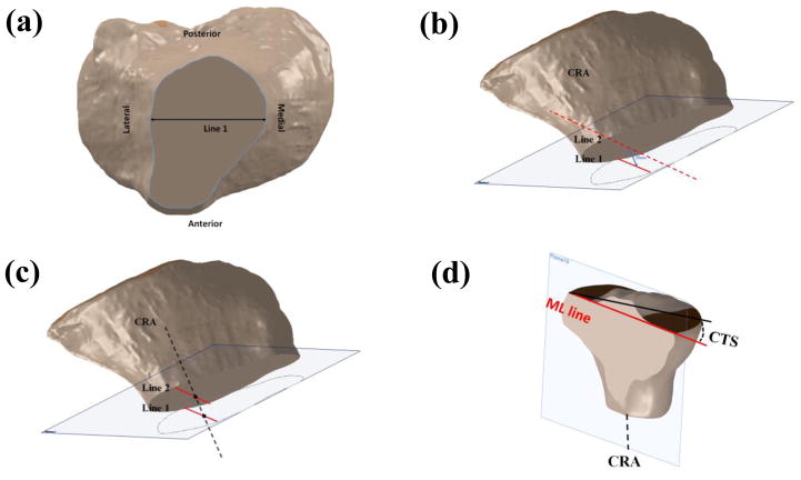
Abstract
Background
The proximal tibia is a geometrically complex, asymmetrical, and variable structure, is heavily implicated in arthrokinematics of the knee joint, and thus impacts weight-bearing knee biomechanics. Such variability and asymmetry may be implicated in knee pathologies such as non-contact anterior cruciate ligament injury.
Medial, lateral, and coronal tibial slopes have been identified as anatomic parameters that may increase predisposition to knee injuries, but the extent to which each contributes has yet to be fully realized. Previously, two-dimensional methods have quantified tibial slopes, but more reliable 3D methods may prove advantageous.
Aims
The aims were: (1) to explore the reliability of two-dimensional methods, (2) to propose a novel three-dimensional measurement approach, and (3) to compare the data derived from traditional and novel methods.
Methods
Medial, lateral, and coronal tibial slope geometry from both knees (left and right) of one subject were obtained via magnetic resonance images and measured by four trained observers from two-dimensional views. The process was repeated via three-dimensional approaches and data were evaluated for intra- and inter- rater reliability.
Results
The conventional method presented a weaker Intraclass Correlation Coefficient (ICC) for the measured slopes (ranging from 0.43 to 0.81) while the resultant ICC for the proposed method indicated greater reliability (ranging from 0.84 to 0.97). Statistical analysis supported the novel three-dimensional approach for production of more reliable and repeatable results for each of the slopes calculated.
Conclusions
The novel three-dimensional method for calculating tibial plateau slope may be more reliable than previously established methods and may provide an important tool during assessment of knee injury risk, susceptibility to osteoarthritis, as part of anterior cruciate ligament injury risk assessment, and in design of total knee implants.
Keywords: imaging, knee, tibial slope, ACL
1. Introduction
The proximal human tibia is a geometrically complex and asymmetrical structure that is heavily implicated in the arthrokinematics of the weight-bearing knee. Geometric variability, including asymmetry, may be implicated in knee pathologies such as increased risk of non-contact anterior cruciate ligament (ACL) injury. While the etiology is multi-factorial, one established key contributor is ACL load-bearing while the knee joint is compressively loaded and experiencing tibial anterior translation and frontal plane valgus moment [1–4]. It has also been well established that ACL injury predisposes individuals to a significantly higher risk of osteoarthritis later in life [5, 6].
Posterior tibial slope (PTS) plays a role in anterior-posterior (AP) stability and translation of the knee joint, and therein has been linked to increased risk of non-contact ACL injury [7–9]. Such risk is likely the result of a direct effect on arthrokinematics, therein yielding increased mechanical tension on the anterior and posterior cruciate ligaments. Recent work has suggested substantial differences between medial and lateral PTS. Hashemi et al. [10] elucidated a divergent risk factor relationship for each, with lateral tibial slope contributing more to increased ACL injury risk than medial slope, particularly for females [8].
Methods for accurate quantitative determination of planar tibial slope measurements have been well documented in the literature. Previous works have established that 2D radiographs (i.e., x-ray images) are not suitable for quantifying tibial slope as they ignore differences in medial vs lateral morphology [10, 11]. With respect to magnetic resonance image (MRI) based calculations, there are various two-dimensional (2D) methods published in the literature to measure tibial slope, notably the work of Hashemi et al. [10, 11] and Giffin et al. [12]. In their collective approaches, a methodology for consistent slope evaluation was established using a reference axis and planar measurements [11, 12].
While the aforementioned efforts have contributed greatly to the field, traditional (2D) approaches suffer measurement error. Measurement error herein is the result of the subjective nature of some of the methodology in conjunction with error associated with 2D imaging assumptions [10]. For instance, the point at which tibial slope is measured along the tibial plateau has traditionally been identified via subjective assessment in an attempt to pick out the center of the diaphysis through visual identification [10]. Accurate and reproducible measurement of the proximal tibial anatomical axis is therefore unlikely with a 2D-based approach [9]. Inconsistencies in slice selection and slice thickness may further compound measurement error when defining tibial slope.
In an effort to improve objective quantitative analysis of MRI-derived tibial slopes, we sought to quantify 2D variability between observers and furthermore demonstrate that lateral and medial tibial slopes vary with respect to the sagittal plane selected for measurement. Additionally, we ventured to demonstrate that coronal tibial slope varies with respect to the frontal plane selected for measurement. Finally, we endeavored to develop a novel approach for three-dimensional (3D) calculation of tibial slopes and to compare the results to those derived via traditional approaches. Our hypothesis was that the proposed novel 3D method would produce more accurate and reliable results. Thus, the specific aims of this study were: (1) to evaluate the reliability of traditional slope calculation methods, (2) to propose a novel 3D measurement approach, and (3) to compare the novel 3D derived data with that obtained via traditional approaches. The results of this study may help elucidate a better understanding of the risk factors for non-contact ACL injury as well as tibial implant alignment in TKA [13–15].
2. Material and methods
After obtaining IRB approval, 3.0 Tesla magnetic resonance (MR) image sequences (Philips Acheiva, Farmington Hills, MI) for both knees of one healthy male subject (2 total) were acquired while the subject was positioned supine, unloaded and neutrally aligned with 1.6 mm slice thickness with 0.8 mm gaps. A turbo field echo sequence with T1 weighting was used for image collection. The subject from whom the images were obtained was a healthy male with a height of 1.82 m and weight of 82.1 kg. This height places the subject at approximately the 75th percentile for the US male population per 2012 US CDC published data [16].
Both sets of scans were evaluated with one 2D and two 3D methods (traditionally-based and novel approach). Subject demographics were obtained and stored in a Health Insurance Portability and Accountability Act (HIPAA) compliant manner. Four trained bioengineering graduate students collected 2D measurements of the lateral, medial, and coronal tibial slopes following the methodological protocol outlined by Hashemi, et al. [11]. The observers repeated each measurement six times for each knee using ImageJ (NIH, Bethesda, MD, USA). The entire process was then repeated via both a 3D approach to the method detailed by Hashemi et al. [11] and a newly proposed 3D method as further outlined in the following sections.
2.1 2D Methodology
2.1.1 Medial and Lateral Tibial Slopes
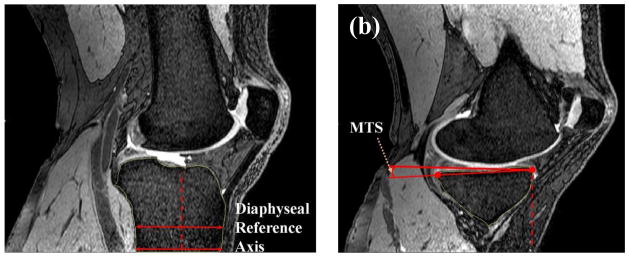
In the sagittal plane, individual image slices were manually reviewed slice-by-slice until the widest section of the tibial diaphysis was determined. While viewing this image in ImageJ, a horizontal line was drawn at the most distal portion of the scan connecting the anterior and posterior tibial cortices, and the midpoint of the line was clearly marked. A second line was drawn 20 mm superiorly to the original line, while still distal to the metaphyseal scar and parallel to the first line. The midpoint of this line was also marked. The midpoints of both lines were connected to represent the longitudinal axis of the tibia as suggested by Hashemi et al [11].
Medially and laterally adjacent slices were then reviewed (moving the image slice viewed to the medial or lateral of the original slice), one slice at a time, until each of the medial and lateral ‘target’ slices were determined. On the medial side, this ‘target slice’ was defined as the slice where the distal portion of the tibial shaft began to subside. On the lateral side, this was defined as the image within which the fibular head first appeared. The line representing the tibial axis was transferred to the superior anterior edge of the tibial plateau and two points were made (one each at the end and middle of the line). The angle between the perpendicular axis and the line created between the anterior and posterior edges of the tibial plateau (Figure 1) was established as the medial (MTS) or lateral (LTS) tibial slope. This process was repeated six times for each knee by each observer for each of the medial and lateral plateaus.
Figure 1.
Definition of the diaphyseal reference axis in sagittal plane (a) based on the methods outlined by Hashemi et al. [11], (b) measurement of the medial tibial slope (MTS) on the target slice.
2.1.2 Coronal Tibial Slope
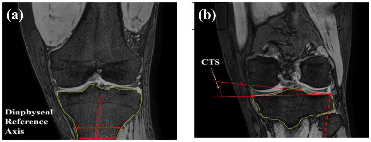
In the coronal plane, images were manually reviewed slice-by-slice until the widest section of the tibial diaphysis was determined. A horizontal line was drawn at the most distal portion of the scan connecting medial and lateral tibial cortices, and the midpoint of the line was marked. A second line 20 mm superior, but distal to the metaphyseal scar, was drawn parallel to the first line and the midpoint of this line was marked. A line connecting the two midpoints was drawn in the same fashion as mentioned in the medial and lateral tibial slope approach.
The line representing the diaphyseal reference axis of the tibia in the coronal plane was then transferred to the superior lateral border of the tibial plateau. The angle between a line perpendicular to the diaphyseal reference axis and the line created between the lateral and medial borders of the tibial plateau was demarked as the coronal tibial slope (CTS). This approach was repeated six times for each knee by each observer (Figure 2).
Figure 2.
Definition of the diaphyseal reference axis in coronal plane (a) based on the methods outlined by Hashemi et al [11], (b) measurement of the coronal tibial slope (CTS) on the target slice.
2.2 3D Methodology
In the 3D approach, the tibia was reconstructed from MR images with Mimics 15.0 (Materialise, Leuven, Belgium) and resultant stereolithographic (STL) files were exported to Geomagic Studio 2014 (3D Systems, North Carolina, USA), wherein image noise and remaining small elements from the MR segmentation process were removed to increase fidelity of the 3D geometry. This was done by eliminating any small gaps and redundant vertices in the STL that may cause poor quality surfaces. The deviation of the resulting shape and the null structure were quantitatively compared (Figure 3).
Figure 3.
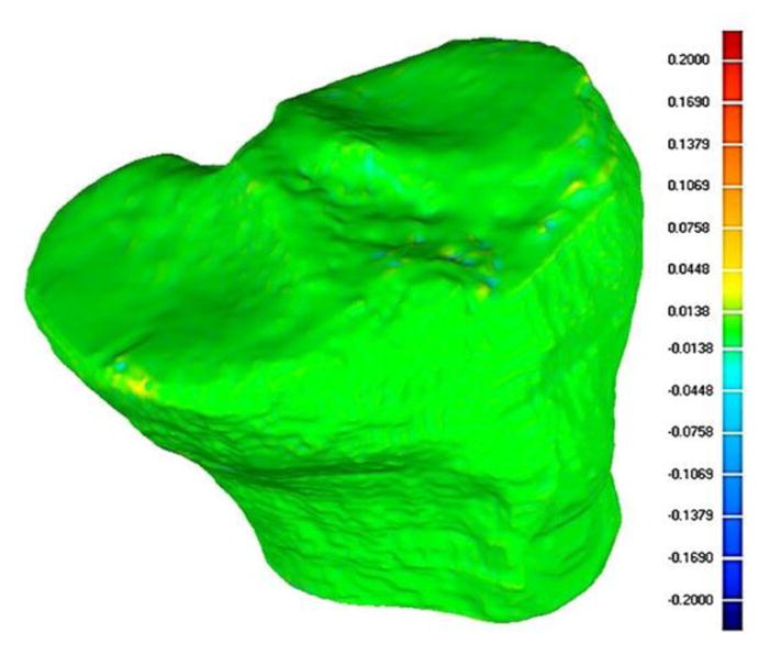
Comparison of the initial STL generated from MR images and the resulting smoothed surface. The figure illustrates less than 0.07 mm deviation from the original structure on the tibial plateau.
If the deviation was accepted (i.e., deviation of the tibial plateau was less than 0.2 mm which equated to 0.335° maximum deviation) Gaussian curvature analysis (70% sensitivity) was performed and the lateral and medial plateaus were defined automatically based on the curvature of the model (Figure 4). The defined surfaces of the tibia were converted to an IGES file and then imported into SolidWorks 2015 (Dassault Systems S.A., Delizy, France) for reference plane fitting and slope calculations (Figure 5).
Figure 4.
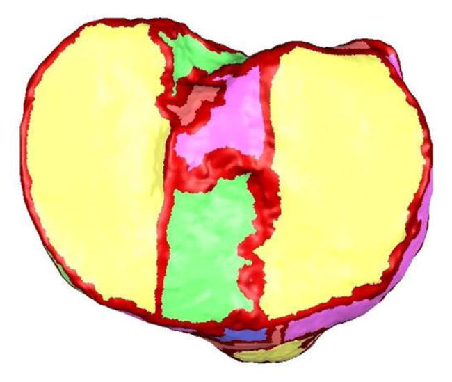
Automatic definition of tibial plateau boundaries based on automated curvature analysis.
Figure 5.
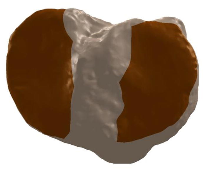
Darker regions denote the borders of the medial and lateral tibial plateaus derived via automated curvature analysis.
3D reconstructions of the tibial samples were performed by one observer and subsequently utilized by all observers. Two methods were utilized for 3D calculation of tibial slopes. The first method was based directly on the approach outlined by Hashemi, et al. [11], adapted to 3D. In the second method, also in 3D, all measurements were made using a novel approach as detailed in section 2.2.1.2 for PTS and section 2.2.2.2 for CTS.
2.2.1 Medial and Lateral Tibial Slope
2.2.1.1 Adapted Hashemi et al. Methodology
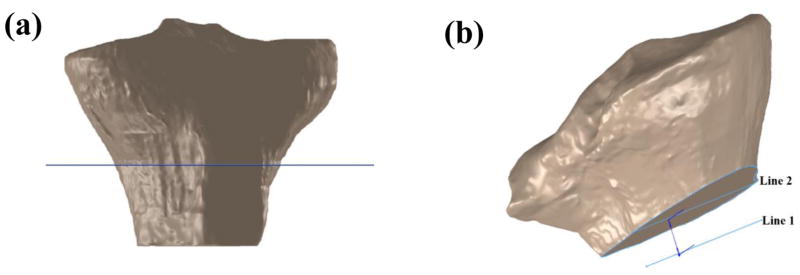
After introducing the STL of the tibia into Solidworks, a transverse plane (plane 1) was passed through the most distal portion of the model. A line (line 1) was drawn across the longest AP dimension of the tibia in plane 1. A second line (line 2) was drawn 20 mm proximal, parallel, and collinear to line 1 within the boundary of the tibia. The sagittal reference axis (SRA) was then defined as the line connecting the midpoints of lines 1 and 2 (Figure 6).
Figure 6.
a) Plane 1 passing through the most distal portion of the tibia. b) Line 1 represents the longest anterior-posterior dimension in the distal tibia. c) Introduction of line 2 collinear, parallel, and 20 mm proximal to line 1.d) Definition of the sagittal reference axis (SRA) after identifying the midpoints of lines 1 and 2 in the 3D adaptation of the methods outlined by Hashemi et al. [11].
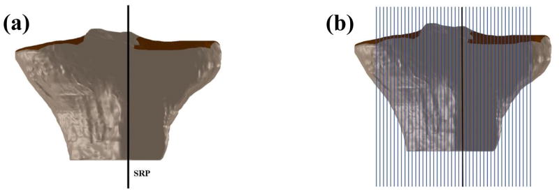
After defining the SRA, a plane coincident with line 2 and perpendicular to plane 1 was introduced as the sagittal reference plane (SRP). Multiple successive planes parallel to the SRP were generated across the entirety of the tibial plateau in 2 mm increments. PTS values were defined as the angles between the lines connecting the anterior and posterior borders of the tibial plateau based on the Gaussian curvature sensitivity analysis and the line perpendicular to the SRA. These measurements were made for each plane across the medial and lateral tibial plateaus (Figure 7). Finally the average slope was reported for each plateau. Each observer repeated this process six times.
Figure 7.
a) Position of the sagittal reference plane (SRP). b) Sagittal planes spaced 2 mm apart starting from the SRP across both the medial and lateral plateaus. c) Sectioned tibia showing measurement of the posterior tibial slope based on the methods outlined by Hashemi et al. [11]
2.2.1.2 Novel 3D Method
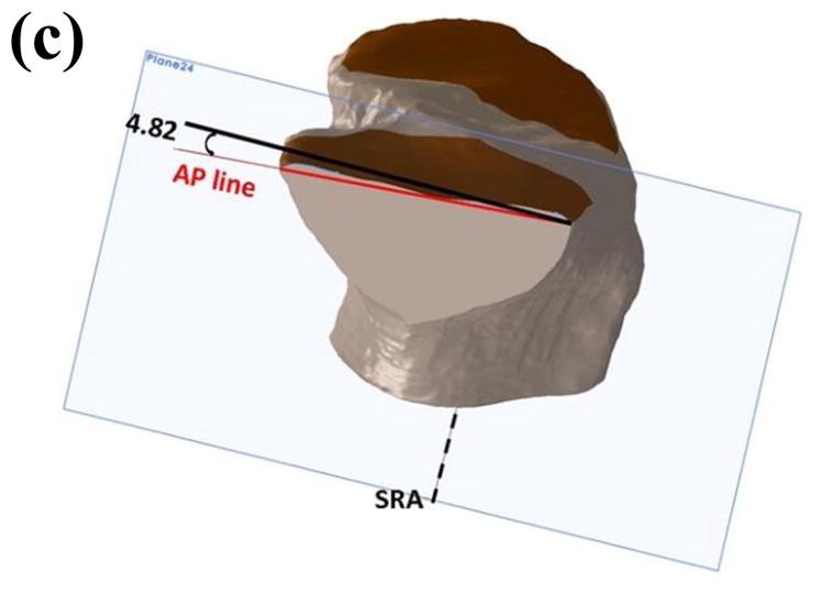
A transversely oriented plane (plane 1) was passed through the most anterior point of the tibial tuberosity. The greatest AP distance was identified in this plane and a line (line 1) was drawn within the tibial borders. Another plane (plane 2) was introduced 20 mm distally to plane 1 and a second line (line 2) was drawn in plane 2 collinear and parallel to line 1 while constrained to the tibial geometry (Figure 8). The midpoints of these lines were connected to define the SRA.
Figure 8.
a) Position of the transverse plane passing through the most anterior point on the tibial tuberosity. b) Lines 1 and 2 passing through the greatest anterior-posterior distance in their respective cross-sections of the tibia.
After defining the SRA, a plane coincident with line 2 and perpendicular to plane 1 was introduced as the SRP (similar to Figure 7a). Successive planes parallel to the SRP were generated across the entirety of the tibial plateau in 2 mm increments (similar to Figure 7b). PTS values were defined as the angle between the lines connecting the anterior and posterior borders, as defined previously by the Gaussian curvature analysis, of the tibial plateau and the line perpendicular to the SRA. These measurements were made for each plane across the medial and lateral tibial plateaus. Finally, the average slope was reported for each plateau. This process was repeated six times by each observer.
2.2.2 Coronal Tibial Slope
2.2.2.1 Adapted Hashemi et al. Methodology
After introducing the STL of the tibia into Solidworks, a plane (plane 1) was passed through the most distal portion of the model. In this plane, a line (line 1) was drawn across the tibia where the medial-lateral (ML) dimension was longest. A second line (line 2) was drawn parallel, collinear, and 20 mm proximally to line 1 while limited to the boundary of the tibia. The coronal reference axis (CRA) was defined as the line connecting the midpoints of lines 1 and 2. A plane collinear with line 2 and perpendicular to plane 1 was introduced as the coronal reference plane (CRP).
After establishing the CRP, successive planes were introduced anteriorly and posteriorly across the tibial plateau in 2 mm increments. The coronal tibial slope (CTS) was defined as the angle between the line connecting the lateral and medial tibial borders and the line perpendicular to the CRA. This measurement was repeated for each plane of interest (Figure 9). Finally, the average slope was reported across the plateau. Each observer repeated this process six times.
Figure 9.
a) Line 1 represents the longest medial-lateral dimension in the distal tibia. b) Introduction of line 2 as collinear, parallel, and 20 mm proximal to line 1. c) Definition of the coronal reference axis (CRA) after identifying the midpoints of lines 1 and 2. d) Sectioned tibia showing measurement of the coronal tibial slope based on the methods outlined by Hashemi et al. [11].
2.2.2.2 Novel 3D method
In the novel 3D approach, a transversely oriented plane (plane 1) was passed through the most anterior point of the tibial tuberosity. The greatest ML distance was identified in this plane and a line (line 1) was drawn within the tibial borders. Another plane was introduced 20 mm distally to plane 1 and a second line (line 2) was drawn collinear and parallel to line 1 while constrained to the tibia geometry. The midpoints of these lines were connected to define the CRA.
After defining the CRA, a plane collinear with line 2 and perpendicular to plane 1 was introduced as the CRP. Successive planes parallel to the CRP were generated across the entirety of the tibial plateau in 2 mm increments. CTS values were defined as the angles between the lines connecting the medial and lateral borders of the tibial plateau based on the Gaussian curvature sensitivity analysis and the line perpendicular to the CRA. These measurements were made for each plane across the tibial plateau. Finally, the average slope was reported across the plateau. Each observer repeated this process six times.
2.3 Statistical Analysis
Means and standard deviations were evaluated and trended for comparison. Intraclass correlation coefficients (ICC) for intra- and inter-rater reliability) were calculated for each observer for each measurement within and across knees (sides) in SPSS 21 (IBM, NY, USA).
3. Results
Overall, evaluation of the slopes calculated in this study revealed marked differences in net mean values derived from each of the three methodologies for medial, lateral, and coronal tibial slopes. Resultant mean slopes were significantly different between methods with alpha set a priori to 0.05. Each of the calculated slopes from the three methods were compared to 75th percentile values statistically interpolated from previously published tibial slope values [8].
3.1 2D Method
The mean of the four observers’ tibial slopes from each plateau of interest based on Hashemi’s work (2D) across observers are presented in Table 1.
Table 1.
2D Hashemi et al. based mean slopes for each slope type and each case. Derived 75th percentile male values [8] are noted for comparison.
| Case ID | Coronal Slope | Medial Slope | Lateral Slope |
|---|---|---|---|
| 1 | 8.1° | 4.1° | 6.8° |
| 2 | 5.9° | 5.8° | 8.5° |
| 75th Percentile | 5.2° | 7.9° | 9.2° |
From an inter-observer standpoint, the calculated tibial slopes showed large variability. As a measure of approach-related accuracy, derived tibial slopes were compared to published ranges derived from the literature [8] and interpolated to values for a 75th percentile male.
ICC results (Table 4) varied for each of the three measured tibial slopes and across methods. ICC results for 2D were 0.810, 0.520, and 0.430 for coronal, medial and lateral tibial slopes, respectively, across four observers and two limbs. IRR results (Table 5) via ICC analysis varied for each of the three measured tibial slopes and across methods. 2D results were 0.527, 0.355, and 0.451 for coronal, medial and lateral tibial slopes, respectively, between four observers.
Table 4.
Intraclass correlation coefficients (ICC) across methods (n=4).
| Method | Coronal Slope | Medial Slope | Lateral Slope |
|---|---|---|---|
| 2D Hashemi-based | 0.810 | 0.520 | 0.430 |
| 3D Hashemi-based | 0.996 | 0.990 | 0.995 |
| 3D Novel | 0.840 | 0.909 | 0.968 |
Table 5.
Inter-Rater Reliability (IRR) across raters (n=4).
| Method | Coronal Slope | Medial Slope | Lateral Slope |
|---|---|---|---|
| 2D Hashemi-based | 0.527 | 0.355 | 0.451 |
| 3D Hashemi-based | 0.996 | 0.989 | 0.992 |
| 3D Novel | 0.828 | 0.909 | 0.958 |
3.2 3D Methods
The mean of the four observers’ tibial slope measurements are presented for the adapted 3D Hashemi method and novel 3D approach in Tables 2 and 3, respectively.
Table 2.
3D Hashemi-based mean slopes for each slope and each case. Derived 75th percentile male values [8] are noted for comparison.
| Case ID | Coronal Slope | Medial Slope | Lateral Slope |
|---|---|---|---|
| 1 | 2.2° | 10.0° | 10.2° |
| 2 | 9.6° | 12.1° | 13.0° |
| 75th Percentile | 5.2° | 7.9° | 9.2° |
Table 3.
Novel approach (3D) mean slopes for each slope and each case. Derived 75th percentile male values [8] are noted for comparison.
| Case ID | Coronal Slope | Medial Slope | Lateral Slope |
|---|---|---|---|
| 1 | 10.3° | 5.3° | 5.1° |
| 2 | 9.3° | 5.3° | 10.5° |
| 75th Percentile | 5.2° | 7.9° | 9.2° |
The 3D measurement approaches provided more reliable measurements for each tibial slope. All but one of the observers recorded similar measurements for the medial and lateral tibial slopes. The results for the coronal tibial slope were more consistent for the observers. The tibial slopes acquired via 2D and 3D measurement approaches were clearly divergent.
ICC results (Table 4) varied for each of the three measured tibial slopes and across methods. ICC results for 3D Hashemi-based were 0.996, 0.990, and 0.995 for coronal, medial and lateral tibial slopes, respectively, across four observers and two limbs.
IRR results (Table 5) via ICC analysis varied for each of the three measured tibial slopes and across methods. 3D Hashemi-based results were 0.996, 0.989, and 0.992 for coronal, medial and lateral tibial slopes, respectively, between four observers.
As for evaluation of the 2D method with respect to reliability, ICC results (Table 4) varied for each of the three measured tibial slopes across methods. ICC results were 0.996, 0.990, and 0.995 for coronal, medial and lateral tibial slopes, respectively, across four observers and two subject limbs for the 3D method based directly on the methods outlined by Hashemi et al. Comparatively, the ICC results were 0.840, 0.909, and 0.968 for coronal, medial and lateral tibial slopes across four observers and two subject limbs for the novel 3D method proposed in this study. It is important to note that established convention states that ICC values greater than 0.70 are considered equivalent to “good” test-retest reliability [17].
As with the 2D data, as a measure of approach-related accuracy, derived tibial slopes were compared to published ranges from the literature [8]. For the 3D approach based on Hashemi’s method, the deviations from published means were 0.6, 3.0, and 2.2 degrees for coronal, medial and lateral tibial slopes, respectively. For the novel 3D approach, deviations from published means were 4.5, −0.2, and −1.6 degrees for coronal, medial and lateral tibial slopes, respectively. ICC results (Table 4) varied for each of the three measured tibial slopes and across methods. ICC results for the 3D novel approach were 0.840, 0.909, and 0.968 for coronal, medial and lateral tibial slopes, respectively, across four observers and two limbs.
IRR results (Table 5) via ICC analysis varied for each of the three measured tibial slopes and across methods. 3D novel approach results were 0.828, 0.909, and 0.958 for coronal, medial and lateral tibial slopes, respectively, between four observers.
4. Discussion
Previous works have established that 2D radiographs (i.e., x-ray images) are not suitable for quantifying tibial slope as they ignore differences in medial vs lateral morphology [10, 11]. With respect to magnetic resonance image (MRI) based calculations, there are various two-dimensional (2D) methods published in the literature to measure tibial slope, notably the work of Hashemi et al [10, 11] and Giffin et al. [12]. In their collective approaches, a methodology for consistent slope evaluation was established using a reference axis and planar measurements [11, 12]. As described in the introduction, traditional (2D) approaches, though potentially applicable, are at risk for measurement error. Even in the hands of trained observers following a regimented protocol, variability is introduced leading to errors in reliability and reproducibility.
In this study, the ICC values for each of the three coronal plane measurement methods were acceptable, as they were all greater than 0.7 [17]. For medial tibial slope, while both of the 3D approaches provided high ICC values, the 2D method performed less favorably (0.527). A similar situation was evident for lateral tibial slope, with both of the 3D methods yielding high ICC values, while the 2D method produced fairly unreliable results (0.43).
Several authors [18–22] have reported values for intra-observer reliability for various 2D approaches similar to those outlined by Hashemi et al. [11] that have herein been compared to two 3D approaches. Hudek et al. [20] used a novel method of 2D determination of tibial slope [23] relying on the fitting of circles to the tibial diaphysis and using the center points of these circles to define the reference axis. The reliability and repeatability of the present study could benefit from the computer-assisted nature of the Hudek et al. approach. Additionally, Hudek et al. commented on the intraclass correlation reported by Hashemi et al. [11], calling into question the validity of their correlation [20], as specifics of the correlation were not outlined in the Hashemi [11] study.
Haddad et al. [19] found strong inter- and intra-class correlations (0.82 and 0.84, respectively) in their study of PTS in different population groups using the proximal tibial anatomical axis. In their effort, specific portions of the tibial plateau (i.e, at center of the whole plateau, in addition to center of the medial and lateral condyles of the tibia) were selected. In our assessment of Hashemi et al.’s approach [11] we did not pre-select slices, but utilized a normalized approach. The standardization of Haddad et al.’s approach [19] coupled with only one observer’s measurements likely impacted the repeatability and reliability of their approach.
Akamatsu et al. found greater reliability and reproducibility of slope calculations via computed topography (CT) images than those from pure radiographic images [18, 22, 23]. However, Akamatsu et al. used nearly full length scans, in addition to short radiographs of the joint space, which included the majority of the tibia and enabled a more accurate determination of tibial slope [24]. Our results were consistent with those of Akamatsu et al. for short radiographs [18]. Although the use of radiographs to measure tibial slope has been contested in the literature due to the superposition of the medial and lateral slopes on each other [22, 25], the reliability and reproducibility in the measurements made by Akamatsu et al. increased with the inclusion of the whole leg in the radiograph.
When accuracy, as measured by deviation of the mean results for each method from the population predicted values for a 75th percentile male, was evaluated for each of the three methods, the 3D methods performed well overall. For coronal tibial slope, the 3D Hashemi method produced results that were closest to the predicted population target [8]. For medial and lateral sagittal tibial slopes (frontal plane), however, the novel 3D method produced values with least deviation from expected results (Table 3).
With respect to study limitations, while there were significant differences in mean tibial slope between the 2D and 3D methods, this was expected as each of the methods used a different tibial vertical axis reference. The methods prescribed by Hashemi et al. [11] referenced the mid-shaft of the tibia which is a function of the scan length of the MRI [24], while the novel 3D method referenced the most anterior point of the tibial tuberosity. Definition of the diaphyseal axis of the tibia inherently introduces error and may therefore yield inconsistent data [26] in a 2D approach. A recent study has shown that placement of the diaphyseal reference axis can vary between observers based, in part, on the length of the distal tibia present in the MR images [26]. Most methods rely on an axis defined by bisecting two lines placed on the distal tibia of the image slice [10–12]. The angle between the axis perpendicular to this plane and a line connecting the anterior-posterior (AP) borders for medial and lateral tibial slope (MTS and LTS, respectively) or medial-lateral (ML) borders for coronal tibial slope (CTS) of the tibia resultantly constitute the tibial slope.
Faschingbauer et al. demonstrated that shorter shaft lengths (akin to shorter scan length) yielded significant variability in slope calculations (a difference of 7.5°) which was a function of the width of the diaphysis present in the scan, therein indicating that the axis is a function of proximal to distal image ‘scan length’ [24]. The location of the reference axis within the scan (i.e., more proximal or distal) also affected the tibial slope measurement. The resultant slope suffers bias accordingly, by no longer being true to the long axis of the tibia, and instead oriented relative only to proximal geometry [11, 22, 25]. This variability and lack of standardization with respect to tibial slope analysis is of clinical concern. Comparison between studies and across different patient populations (i.e., ethnicities) is resultantly difficult given different approach methodologies and observers [19]. A dependence on image ‘scan length’ can therein lead to misalignment of the tibial axis, producing potentially misleading slope measurements.
The authors recognize that the small sample size in this study (two knees from one subject) reduced statistical power. However, we feel that the results of the novel approach, and the application of the method outlined by Hashemi et al. [11] show promise for the development and deployment of more comprehensive means to evaluate tibial slope.
Finally, the authors are cognizant that the current approach, while enhanced, is still not easily and intuitively deployed by most clinicians. Future efforts should apply the methods developed in this study to more rapid and efficient computational methods, such as computer vision algorithm approaches, in order to promote clinical adoption through a custom-developed software package. Future work encompassing larger sample sizes should also evaluate statistical relationships between each of the tibial slopes, highlight the slice by slice variability within subjects as compared with single site or mean slope values, assess the strength of various approaches for determining and the slope of the proximal tibia, and correlate 3D relevant geometries with 2D image calculations as a surrogate.
5. Conclusions
While the repeatability and accuracy results of this study provide support in favor of adopting 3D methods for coronal and sagittal tibial slope calculation, the researchers herein realize that computational efficiency and clinical ease of use are important factors to consider. Thus, while the newly introduced methodology shows promise, it is not without limitations and is not yet rapid enough to be widely supported in the clinical environment.
The proposed novel 3D method for calculating tibial plateau slope shows promise for providing a more reliable method than previously substantiated 2D methods. The 3D measurement method introduced in this work may ultimately prove useful as a tool for accurate assessment of geometric variability at the knee with respect to evaluating osteoarthritis susceptibility, as part of ACL injury risk assessment, and in the design of total knee implants.
Highlights.
Geometric variability of the proximal tibia may be implicated in knee injury risk.
Comparing results between studies introduces error without standardized methods.
This approach may provide a more reliable and computationally efficient method.
Acknowledgments
Work supported in part by the National Institutes of Health (R01 AR056259-06-TEH).
Abbreviations
- ACL
anterior cruciate ligament
- AP
anterior-posterior
- CRA
coronal reference axis
- CRP
coronal reference plane
- CT
computed topography
- CTS
coronal tibial slope
- LTS
lateral tibial slope
- ML
medial-lateral
- MRI
magnetic resonance image
- MTS
medial tibial slope
- PTS
posterior tibial slope
- SRA
sagittal reference axis
- SRP
sagittal reference plane
- STL
stereolithographic
- HIPAA
Health Insurance Portability and Accountability Act
- ICC
Intraclass Correlation Coefficients
- IRR
Inter Rater Reliability
- 2D
two-dimensional
- 3D
three-dimensional
Footnotes
Publisher's Disclaimer: This is a PDF file of an unedited manuscript that has been accepted for publication. As a service to our customers we are providing this early version of the manuscript. The manuscript will undergo copyediting, typesetting, and review of the resulting proof before it is published in its final citable form. Please note that during the production process errors may be discovered which could affect the content, and all legal disclaimers that apply to the journal pertain.
References
- 1.Hewett TE, Lindenfeld TN, Riccobene JV, Noyes FR. The effect of neuromuscular training on the incidence of knee injury in female athletes a prospective study. The American journal of sports medicine. 1999;27:699–706. doi: 10.1177/03635465990270060301. [DOI] [PubMed] [Google Scholar]
- 2.Hewett TE, Myer GD, Ford KR. Anterior cruciate ligament injuries in female athletes part 1, mechanisms and risk factors. The American journal of sports medicine. 2006;34:299–311. doi: 10.1177/0363546505284183. [DOI] [PubMed] [Google Scholar]
- 3.Meyer EG, Baumer TG, Slade JM, Smith WE, Haut RC. Tibiofemoral contact pressures and osteochondral microtrauma during anterior cruciate ligament rupture due to excessive compressive loading and internal torque of the human knee. The American journal of sports medicine. 2008;36:1966–77. doi: 10.1177/0363546508318046. [DOI] [PubMed] [Google Scholar]
- 4.Fleming BC, Renstrom PA, Beynnon BD, Engstrom B, Peura GD, Badger GJ, et al. The effect of weight bearing and external loading on anterior cruciate ligament strain. Journal of biomechanics. 2001;34:163–70. doi: 10.1016/s0021-9290(00)00154-8. [DOI] [PubMed] [Google Scholar]
- 5.Gabriel MT, Wong EK, Woo SLY, Yagi M, Debski RE. Distribution of in situ forces in the anterior cruciate ligament in response to rotatory loads. Journal of Orthopaedic Research. 2004;22:85–9. doi: 10.1016/S0736-0266(03)00133-5. [DOI] [PubMed] [Google Scholar]
- 6.Lohmander L, Östenberg A, Englund M, Roos H. High prevalence of knee osteoarthritis, pain, and functional limitations in female soccer players twelve years after anterior cruciate ligament injury. Arthritis & Rheumatism. 2004;50:3145–52. doi: 10.1002/art.20589. [DOI] [PubMed] [Google Scholar]
- 7.Beynnon BD, Hall JS, Sturnick DR, DeSarno MJ, Gardner-Morse M, Tourville TW, et al. Increased Slope of the Lateral Tibial Plateau Subchondral Bone Is Associated With Greater Risk of Noncontact ACL Injury in Females but Not in Males A Prospective Cohort Study With a Nested, Matched Case-Control Analysis. The American journal of sports medicine. 2014;42:1039–48. doi: 10.1177/0363546514523721. [DOI] [PMC free article] [PubMed] [Google Scholar]
- 8.Whitney DC, Sturnick DR, Vacek PM, DeSarno MJ, Gardner-Morse M, Tourville TW, et al. Relationship Between the Risk of Suffering a First-Time Noncontact ACL Injury and Geometry of the Femoral Notch and ACL A Prospective Cohort Study With a Nested Case-Control Analysis. The American journal of sports medicine. 2014 doi: 10.1177/0363546514534182. 0363546514534182. [DOI] [PMC free article] [PubMed] [Google Scholar]
- 9.Stijak L, Herzog RF, Schai P. Is there an influence of the tibial slope of the lateral condyle on the ACL lesion? Knee surgery, sports traumatology, arthroscopy. 2008;16:112–7. doi: 10.1007/s00167-007-0438-1. [DOI] [PubMed] [Google Scholar]
- 10.Hashemi J, Chandrashekar N, Mansouri H, Gill B, Slauterbeck JR, Schutt RC, et al. Shallow medial tibial plateau and steep medial and lateral tibial slopes new risk factors for anterior cruciate ligament injuries. The American journal of sports medicine. 2010;38:54–62. doi: 10.1177/0363546509349055. [DOI] [PubMed] [Google Scholar]
- 11.Hashemi J, Chandrashekar N, Gill B, Beynnon BD, Slauterbeck JR, Schutt RC, et al. The geometry of the tibial plateau and its influence on the biomechanics of the tibiofemoral joint. The Journal of Bone & Joint Surgery. 2008;90:2724–34. doi: 10.2106/JBJS.G.01358. [DOI] [PMC free article] [PubMed] [Google Scholar]
- 12.Giffin JR, Vogrin TM, Zantop T, Woo SL, Harner CD. Effects of increasing tibial slope on the biomechanics of the knee. The American journal of sports medicine. 2004;32:376–82. doi: 10.1177/0363546503258880. [DOI] [PubMed] [Google Scholar]
- 13.Stindel E, Briard J, Merloz P, Plaweski S, Dubrana F, Lefevre C, et al. Bone morphing: 3D morphological data for total knee arthroplasty. Computer Aided Surgery. 2002;7:156–68. doi: 10.1002/igs.10042. [DOI] [PubMed] [Google Scholar]
- 14.Andani MT, Moghaddam NS, Haberland C, Dean D, Miller MJ, Elahinia M. Metals for bone implants. Part 1. Powder metallurgy and implant rendering. Acta biomaterialia. 2014;10:4058–70. doi: 10.1016/j.actbio.2014.06.025. [DOI] [PubMed] [Google Scholar]
- 15.Mensch JS, Amstutz H. Knee morphology as a guide to knee replacement. Clinical Orthopaedics and Related Research. 1975:231–41. [PubMed] [Google Scholar]
- 16.Fryar CD, Gu Q, Ogden CL. Anthropometric reference data for children and adults: United States, 2007–2010. Vital and health statistics Series 11, Data from the national health survey. 2012:1–48. [PubMed] [Google Scholar]
- 17.de Vet HC, Terwee CB, Knol DL, Bouter LM. When to use agreement versus reliability measures. Journal of clinical epidemiology. 2006;59:1033–9. doi: 10.1016/j.jclinepi.2005.10.015. [DOI] [PubMed] [Google Scholar]
- 18.Akamatsu Y, Sotozawa M, Kobayashi H, Kusayama Y, Kumagai K, Saito T. Usefulness of long tibial axis to measure medial tibial slope for opening wedge high tibial osteotomy. Knee Surgery, Sports Traumatology. Arthroscopy. 2014:1–7. doi: 10.1007/s00167-014-3403-9. [DOI] [PubMed] [Google Scholar]
- 19.Haddad B, Konan S, Mannan K, Scott G. Evaluation of the posterior tibial slope on MR images in different population groups using the tibial proximal anatomical axis. Acta orthopaedica Belgica. 2012;78:757. [PubMed] [Google Scholar]
- 20.Hudek R, Fuchs B, Regenfelder F, Koch P. Is noncontact ACL injury associated with the posterior tibial and meniscal slope? Clinical Orthopaedics and Related Research®. 2011;469:2377–84. doi: 10.1007/s11999-011-1802-5. [DOI] [PMC free article] [PubMed] [Google Scholar]
- 21.Lipps DB, Wilson AM, Ashton-Miller JA, Wojtys EM. Evaluation of different methods for measuring lateral tibial slope using magnetic resonance imaging. The American journal of sports medicine. 2012;40:2731–6. doi: 10.1177/0363546512461749. [DOI] [PMC free article] [PubMed] [Google Scholar]
- 22.Utzschneider S, Goettinger M, Weber P, Horng A, Glaser C, Jansson V, et al. Development and validation of a new method for the radiologic measurement of the tibial slope. Knee Surgery, Sports Traumatology, Arthroscopy. 2011;19:1643–8. doi: 10.1007/s00167-011-1414-3. [DOI] [PubMed] [Google Scholar]
- 23.Hudek R, Schmutz S, Regenfelder F, Fuchs B, Koch PP. Novel measurement technique of the tibial slope on conventional MRI. Clinical Orthopaedics and Related Research®. 2009;467:2066–72. doi: 10.1007/s11999-009-0711-3. [DOI] [PMC free article] [PubMed] [Google Scholar]
- 24.Faschingbauer M, Sgroi M, Juchems M, Reichel H, Kappe T. Can the tibial slope be measured on lateral knee radiographs? Knee Surgery, Sports Traumatology, Arthroscopy. 2014;22:3163–7. doi: 10.1007/s00167-014-2864-1. [DOI] [PubMed] [Google Scholar]
- 25.Yoo JH, Chang CB, Shin KS, Seong SC, Kim TK. Anatomical references to assess the posterior tibial slope in total knee arthroplasty: a comparison of 5 anatomical axes. The Journal of arthroplasty. 2008;23:586–92. doi: 10.1016/j.arth.2007.05.006. [DOI] [PubMed] [Google Scholar]
- 26.Sheehy L, Felson D, Zhang Y, Niu J, Lam Y-M, Segal N, et al. Does measurement of the anatomic axis consistently predict hip-knee-ankle angle (HKA) for knee alignment studies in osteoarthritis? Analysis of long limb radiographs from the multicenter osteoarthritis (MOST) study. Osteoarthritis and Cartilage. 2011;19:58–64. doi: 10.1016/j.joca.2010.09.011. [DOI] [PMC free article] [PubMed] [Google Scholar]


