Transfer Learning with Convolutional Neural Networks for Classification of Abdominal Ultrasound Images

Abstract

The purpose of this study is to evaluate transfer learning with deep convolutional neural networks for the classification of abdominal ultrasound images. Grayscale images from 185 consecutive clinical abdominal ultrasound studies were categorized into 11 categories based on the text annotation specified by the technologist for the image. Cropped images were rescaled to 256 × 256 resolution and randomized, with 4094 images from 136 studies constituting the training set, and 1423 images from 49 studies constituting the test set. The fully connected layers of two convolutional neural networks based on CaffeNet and VGGNet, previously trained on the 2012 Large Scale Visual Recognition Challenge data set, were retrained on the training set. Weights in the convolutional layers of each network were frozen to serve as fixed feature extractors. Accuracy on the test set was evaluated for each network. A radiologist experienced in abdominal ultrasound also independently classified the images in the test set into the same 11 categories. The CaffeNet network classified 77.3% of the test set images accurately (1100/1423 images), with a top-2 accuracy of 90.4% (1287/1423 images). The larger VGGNet network classified 77.9% of the test set accurately (1109/1423 images), with a top-2 accuracy of VGGNet was 89.7% (1276/1423 images). The radiologist classified 71.7% of the test set images correctly (1020/1423 images). The differences in classification accuracies between both neural networks and the radiologist were statistically significant (p < 0.001). The results demonstrate that transfer learning with convolutional neural networks may be used to construct effective classifiers for abdominal ultrasound images.

Introduction

Classification of images by anatomic or pathologic features is a fundamental cognitive task in diagnostic radiology. Although computers are currently far from being able to reproduce the full chain of reasoning required for medical image interpretation, the automation of basic image classification is a focus of research in computer vision, a multidisciplinary field that incorporates ideas from image processing, machine learning, and neuroscience. A digital image can be regarded as a matrix of numbers encoding the brightness and color of individual pixels. An image classification algorithm typically reduces this matrix into a simpler vector of image features such as edges, curves, blobs, and textures. These features in turn can be combined to encode larger scale features such as the identity, shape, orientation, and environment of objects. Until recently, improvements in automated image classification relied heavily on engineering of hand-crafted image features for discriminating the image categories of interest.

A branch of machine learning termed “deep learning” has recently provided breakthrough performance improvements in diverse tasks including image classification, object detection, speech recognition, natural language processing, and game playing [1–4]. A deep learning system most commonly uses a multilayer artificial neural network, an arrangement of mathematically interconnected nodes inspired by biological neural networks. Neural networks have a long history in machine learning, including various applications in radiology, e.g., [5–7]. However, “deep” neural networks feature hierarchical multilayer architectures allowing them to learn not only the mappings of data features to categories but also the features themselves [1]. For effective training, these systems have benefited from the recent availability of large amounts of labeled input data as well as improvements in computing power.

For image classification, convolutional neural networks have proven particularly effective in processing raw pixel data. These networks employ a hierarchical topology of connections inspired by biological visual systems, whereby low level nodes in the network process a spatially limited grid of pixels, and higher level nodes encode increasingly complex features by combining simpler features from lower levels. Weights are shared among nodes in the same layer in a manner allowing recognition of the same image motif in any number of spatial positions. Convolutional neural networks of increasing depth and complexity have been used to advance the state of the art in image classification. This has been most visibly demonstrated by recent winning entries in the ImageNet Large Scale Visual Recognition Challenge (ILSVRC) [8–10], an annual competition in object recognition based on a dataset of over a million images in hundreds of object categories [11].

As convolutional neural networks have become widely used in image classification, there has been increasing interest in evaluating the use of these networks in medical imaging [4, 12–16]. However, slow adoption of convolutional neural networks in radiology is partly due to the relative lack of large labeled medical image data sets for training and testing. In this work, we employ transfer learning [13, 14, 17, 18] to partially overcome the problem of relatively small medical image datasets. Specifically, we re-trained two large convolutional neural networks, originally trained to classify color photographs for the ImageNet Large Scale Visual Recognition Challenge, to classify a set of clinical greyscale abdominal ultrasound images. We hypothesize that the pre-trained weights of these convolutional neural networks can serve as an effective image recognition baseline for classification of ultrasound images.

Materials and Methods

Institutional Review Board approval was obtained for the retrospective data collection and analysis in this study.

Ultrasound Images

A total of 9298 grayscale images from 185 consecutive clinical abdominal ultrasound studies performed on distinct patients (108 male and 77 female) from August to December 2015 were retrospectively obtained from the picture archival and communications system (PACS). Ninety-eight studies were obtained from a Philips EPIQ 7G ultrasound scanner, and 87 studies from a Toshiba Aplio XG scanner. Patient ages ranged from 20 to 78 years (mean ± SD, 53 ± 13 years). The studies were performed for a variety of indications, but many (101 studies) were performed in patients with end-stage renal disease, for pre-transplant screening (Table 1).

Table 1.

Clinical indications for the abdominal ultrasound studies used for training and testing the neural networks

Indication	Number of studies
End stage renal disease (pre-transplant)	101
Elevated liver function tests	22
Tumor evaluation/surveillance	20
Abdominal pain	14
Organ size assessment	5
Other	23
Total	185

All images were obtained using curved array transducers. The images were categorized into 11 categories based on the text annotation specified by the technologist for the image. Images that did not fall into any of the 11 categories were excluded. In addition, images were excluded that employed color or spectral Doppler, or contained any superimposed annotations or measurements. Finally, images were excluded which were thought to have very limited or no recognizable anatomy of the labeled target organ. The classifications and exclusions were performed and reviewed by an abdominal radiologist with 7 years of post-fellowship clinical experience. A total of 5518 images remained, with category statistics given in Table 2.

Table 2.

Categories of images in the training and test sets

Category	Training set	Test set	Total images
Liver left longitudinal	482 (11.8%)	191 (13.4%)	673 (12.2%)
Liver left transverse	464 (11.3%)	164 (11.5%)	628 (11.4%)
Liver right longitudinal	531 (13.0%)	171 (12.0%)	702 (12.7%)
Liver right transverse	653 (15.9%)	223 (15.7%)	876 (15.9%)
Spleen	137 (3.3%)	48 (3.4%)	185 (3.4%)
Pancreas	273 (6.7%)	104 (7.3%)	377 (6.8%)
Kidney left longitudinal	183 (4.5%)	65 (4.6%)	248 (4.5%)
Kidney left transverse	318 (7.8%)	99 (7.0%)	417 (7.6%)
Kidney right longitudinal	193 (4.7%)	67 (4.7%)	260 (4.7%)
Kidney right transverse	285 (7.0%)	93 (6.5%)	378 (6.9%)
Gallbladder	576 (14.1%)	198 (13.9%)	774 (14.0%)
Total	4095	1423	5518

Each image was cropped to a central square for use in the training and test sets in order to exclude surrounding text and graphics annotations. The sizes of the crop squares were determined by the resolution of the images for each ultrasound scanner, and the maximum square that could be used without including surrounding text or graphical annotations. Specifically, the crop squares measured 600 × 600 pixels for the Philips scanner images (from 1024 × 768 pixel source images) and 372 × 372 pixels for the Toshiba scanner images (from 716 × 537 pixel source images). Each grayscale image was then downsampled and saved in a 256 × 256 resolution in 24-bit RGB JPEG format to fit the size of the 3-channel input layers of the neural networks.

The 185 studies were randomized with 4094 images from 136 studies constituting the training set, and 1423 images from 49 studies constituting the test set. Images were grouped by study in the randomization in order to keep potentially correlated images together. As shown in Table 2, the category distributions for the training and test set images were similar, reflecting the category distribution for images in a typical abdominal ultrasound study.

Neural Networks

For training and testing the neural networks, we used the open source deep learning framework Caffe [19]. All training and testing was performed on a Windows 64-bit desktop personal computer with an Intel Core i7 4770 central processing unit (CPU), 8 GB random access memory, and no graphical processing unit (GPU).

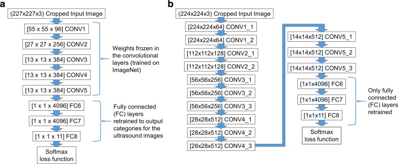
The first neural network architecture we used is CaffeNet [20], a modified version of the AlexNet winning architecture used in the ILSVRC 2012 competition [8]. The network consists of 5 convolutional layers (CONV1 to CONV5) followed by 3 fully connected layers (FC6 to FC8) and a softmax (multinomial logistic regression) classifier (Fig. 1a). We used publicly available weights for the network [20], trained against the ILSVRC12 challenge data set. The final fully connected layer FC8 was replaced with a layer with 11 outputs corresponding to the 11 image categories, and initialized with random weights. For training, the weights for the five convolutional layers were frozen to serve as a feature extractor. We used a batch size of 256 images for each iteration of training. The learning rates for the fully connected FC6, FC7, and FC8 layers were fixed at 0.001, 0.001, and 0.01 respectively during training, allowing learning to occur faster for the final fully connected layer (FC8). For each image, a training set mean image was subtracted, and random 227 × 227 pixel crops of the 256 × 256 pixel input images were used to match the dimensions of the input layer (the random crops provide a degree of data augmentation for training).

Fig. 1.

Layer structures of the modified a CaffeNet and b VGGNet neural networks used in the study. Numbers in brackets indicate the number of nodes within a layer of the neural network. CONV = convolutional layer, FC = fully connected layer

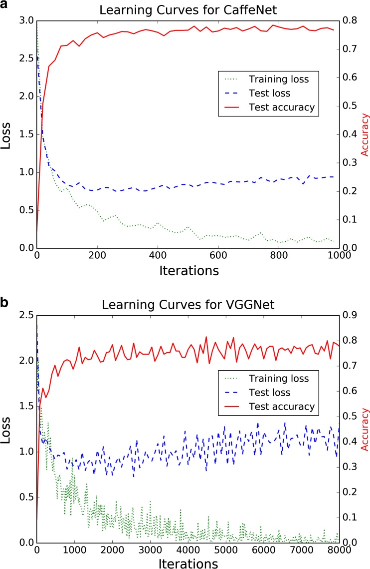
Training was set to occur over 1000 iterations (62.5 training epochs), which required approximately 2.5 h. The cross-entropy loss function for the training batches reached a low plateau toward the end of training (Fig. 2a). For each test image, the training set mean image is subtracted, and fixed central 227 × 227 pixel crops of the 256 × 256 pixel input images are used in the input layer of the network. Test set classification required an average of 0.10 s per image.

Fig. 2.

Learning curves for a CaffeNet and b VGGNet. Loss curves indicate the training cross-entropy loss as a function of the training iteration. The test curves provide information on the loss function and classification accuracy of the test set during training, but were not used to optimize training hyperparameters

The second neural network architecture we used is a modified version of the 16-layer model from the VGG team in the ILSVRC-2014 competition (denoted as configuration D in [9]); in our study, we denote it as VGGNet. The network consists of 13 convolutional layers followed by 3 fully connected layers (FC6 to FC8) and a softmax classifier (Fig. 1b). We used publicly available weights for the network [21], trained against the ILSVRC12 challenge data set.

As with the CaffeNet network, the final fully connected layer FC8 in VGGNet was replaced with a layer with 11 outputs, initialized with random weights. For training, the weights for the 13 convolutional layers were frozen to serve as a feature extractor. Due to the larger size and memory requirements of this model compared to CaffeNet, we used a batch size of 32 images for each iteration of training (1/8 the batch size for CaffeNet). To provide training comparable to CaffeNet, the learning rates for the fully connected FC6, FC7, and FC8 layers were fixed at 1/8 the value for the CaffeNet training (0.000125, 0.000125, and 0.00125, respectively), but for 8 times the number of iterations (8000 iterations, equivalent to 62.5 training epochs given the smaller batch size). For each image, the training set mean image was subtracted, and random 224 × 224 pixel crops of the 256 × 256 pixel input images were used to match the input dimensions of the input layer. Note that we used mean image subtraction instead of the mean pixel subtraction used in the original VGGNet description [9], due to the consistent sector shape of input image data resulting from the ultrasound curved array transducers.

Training for the 8000 iterations required approximately 27.5 h. The cross-entropy loss function for the training batches reached a low level toward the end of training, though with more pronounced oscillations compared to CaffeNet (Fig. 2b). For each test image, the training set mean image was subtracted, and fixed central 224 × 224 pixel crops of the 256 × 256 pixel input images were used in the input layer of the network. Test set classification required an average of 0.52 s per image.

For both neural networks, the softmax classifier provides a probability for each of the 11 categories for a given input image. The category with the highest predicted probability was taken as the classifier prediction for the image, and we calculated classification accuracy based on this prediction (top-1 accuracy). We also calculated top-2 accuracy for each network on the test set, using the highest two probability classes for each image as the classifier prediction.

Both of the convolutional nets can be regarded as transforming the input images into 4096-dimensional vectors (the size of the last fully connected layer FC7 before the classifier). In order to better visualize the classification behavior of the networks, we calculated the FC7 vector representations of the images of the training set, and reduced them to 50 dimensions using principal components analysis (PCA). We then further reduced the dimensionality of these 50-dimensional vectors to two dimensions using t-distributed stochastic neighbor embedding (t-SNE), a machine learning technique which reduces dimensionality while tending to preserve pairwise Euclidean distances between data points [22]. We used the scikit-learn open source implementations of both PCA and t-SNE [23].

Human Classifier

The human classifier for this study was a fellowship-trained abdominal radiologist with 5 years of post-fellowship experience, who spends more than 50% of his clinical time in diagnostic ultrasound, and who is familiar with the abdominal ultrasound protocol performed by the technologists in this study. This radiologist had previously dictated 4 studies from the training set and 1 study from the test set; these ultrasound studies had been performed and dictated more than 5 months prior to the classification task required for this study. A custom graphical user interface allowed browsing of classified images in the training set and shortcut-enabled manual classification of the images in the test set. The order of the test set images was randomized. The total amount of time required to classify the test set, over several sessions, was approximately 12 h.

Statistical Analysis

Comparisons between the classification accuracies of the two neural networks, as well as between the radiologist and each network, were performed with χ ² tests with a p value of 0.05 or less taken to indicate a statistically significant difference. The calculations were performed using the R statistical environment, version 3.30 [24].

Results

After training, the convolutional neural network based on CaffeNet classified 99.8% of the training set accurately (4088/4095 images). The convolutional neural network based on VGGNet classified 100% of the training set accurately (4095/4095 images).

On the test set, the Caffenet network classified 77.3% of the images accurately (1100/1423 images). Considering the top 2 candidate classes for each image (top-2 accuracy), the network’s accuracy is 90.4% (1287/1423 images). By comparison, the larger VGGNet network classifies 77.9% of the test set accurately (1109/1423 images). The top-2 accuracy of VGGNet was 89.7% (1276/1423 images). The classification accuracies of the two neural networks were not significantly different, with χ ² (df = 1) = 0.129, p = 0.719.

Classification accuracies for CaffeNet on images acquired on the Toshiba scanner versus the Philips scanner were slightly different at 73.8% (432/585 images) and 79.7% (668/838 images), respectively, with χ ² (df = 1) = 6.43, p = 0.011. On the other hand, classification accuracies for VGGNet on images acquired on the Toshiba scanner versus the Philips scanner were similar at 77.4% (453/585 images) and 78.3% (656/838 images), respectively, with χ ² (df = 1) = 0.10, p = 0.75.

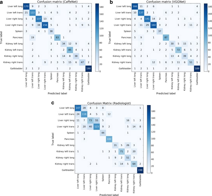
Confusion matrices for the CaffeNet network on the test set of images (Fig. 3) show that the largest sources of error were in distinguishing between transverse and longitudinal images of the liver, between views of the left and right kidney, and between pancreas images and transverse views of the left hepatic lobe. The VGGNet network performed slightly better than CaffeNet on distinguishing transverse and longitudinal images of the left hepatic lobe, and distinguishing pancreas views from transverse views of the left hepatic lobe.

Fig. 3.

Confusion matrices for a CaffeNet, b VGGNet, and c an ultrasound radiologist. Numbers in each box indicate the number of images corresponding to each combination of predicted and true labels. Counts of correctly labeled images are along the diagonal

The radiologist classified 71.7% of the test set images correctly (1020/1423 images). The difference between the radiologist classification accuracy and the classification accuracies of the neural networks was statistically significant. Comparing the radiologist and CaffeNet, χ ² (df = 1) = 11.54, p < 0.001. Comparing the radiologist and VGGNet, χ ² (df = 1) = 14.44, p < 0.001.

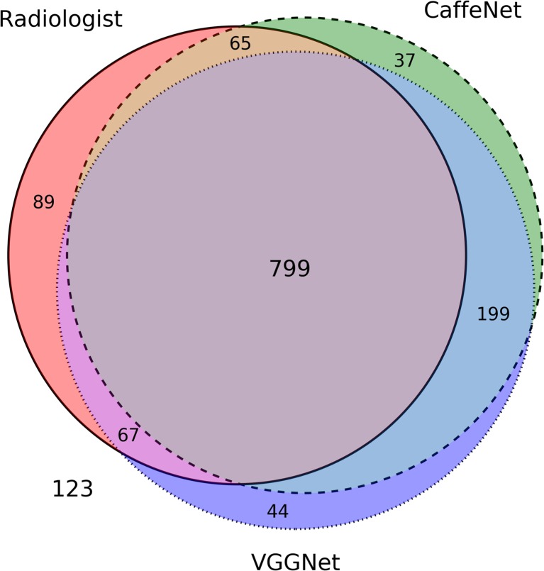
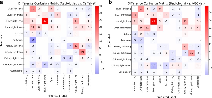
A Venn diagram of correctly classified images in the test set shows significant overlap among images correctly classified by the radiologist and two neural networks (Fig. 4). Difference confusion matrices for the radiologist relative to CaffeNet or VGGNet (Fig. 5) show that an outlier source of excess error for the radiologist was in distinguishing between longitudinal and transverse images of the right hepatic lobe, and in distinguishing between longitudinal and transverse images of the left hepatic lobe. If the excess radiologist error from these images compared to CaffeNet was eliminated, the radiologist’s classification accuracy would be 76.6%. Alternatively, if the excess radiologist error from these images compared to VGGNet was eliminated, the radiologist’s accuracy would be 77.5%.

Fig. 4.

Venn diagram for images correctly classified by the two neural networks (CaffeNet = dashed circle, VGGNet = dotted circle) and the radiologist (solid circle). The areas of the diagram are approximately proportional to the number of images; the large common area in the center represents the 799 images classified correctly by both neural networks and the radiologist. A total of 123 images were incorrectly classified by both neural networks and the radiologist

Fig. 5.

Difference confusion matrices comparing incorrectly classified images between a the radiologist and CaffeNet and b the radiologist and VGGNet. Positive numbers indicate excess errors by the radiologist compared to the neural networks; negative numbers indicate excess errors by the neural networks compared to the radiologist. For clarity, counts of correctly classified images along the diagonal are omitted

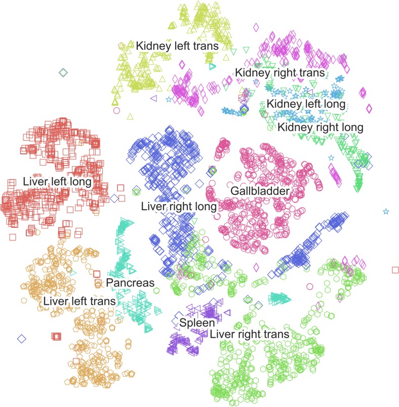
A t-SNE plot for CaffeNet (Fig. 6) depicts the distribution of two-dimensional representations of the 4096-element vectors to which the training images are mapped in the last fully connected layer (FC7). The plot demonstrates areas of overlap that correspond to classification confusion categories on the test set images. For instance, there is significant overlap between the representations of the longitudinal views of the left and right kidney, and of longitudinal and transverse images of the right hepatic lobe.

Fig. 6.

Visualization by t-SNE of CaffeNet’s high dimensional vector representations of the 4094 training set images. Images with a similar high dimensional vector representation are displayed close to each other in this map

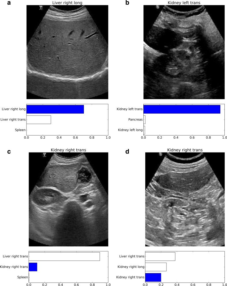
Examples of misclassified images are shown in Fig. 7.

Fig. 7.

Examples of misclassified images. The correct technologist label appears above each image; the bar graph below each image depicts the top three category probabilities given by the CaffeNet network, with the dark bar corresponding to the correct image label. Images (a) and (b) were incorrectly classified by the radiologist but correctly classified by both neural networks. Images (c) and (d) were correctly classified by the radiologist but incorrectly classified by both neural networks

Discussion

This study demonstrates that deep convolutional neural networks trained to classify color nonmedical photographs can be retrained to classify greyscale abdominal ultrasound images. In particular, the convolutional layer features of these networks can be used as unmodified feature extractors for classifying ultrasound images, despite the contrasting image noise texture and lack of color information in the ultrasound images. At the same time, the fully connected layers of these networks are sufficiently flexible to be retrained on a very different image set.

Through transfer learning, we were able to train both neural networks with a relatively small amount of training data—4094 grayscale ultrasound images, versus the more than 1.4 million images in the ILSVRC data set [11]. As we did not evaluate classification accuracy as a function of training set size, it is possible that the training set could have been even smaller without severely impacting classification performance [12]. In any case, we believe that the success of transfer learning in this study is promising for the prospect of training convolutional neural networks for other medical imaging tasks, where the availability of large image data sets with concise labels may be similarly limited.

The image classification task in this study is based on clinical diagnostic grayscale abdominal ultrasound images with readily available ground truth labels. Some image label ambiguity arises from the fact that these labels were assigned by the ultrasound technologist to describe a particular diagnostic view, rather than the specific anatomy within a given image. Certain image labels were challenging to reconstruct because different ultrasound views may overlap. Other image labels were uncertain because of a lack of distinctive anatomic features in a given image to specify a particular view. For instance, our study population included a disproportionately high number of patients with atrophic kidneys with poorly distinguishable renal parenchyma.

We felt that it was important to retain these labeling challenges from the training and test sets in order for them to constitute a realistic sample of clinical images. In order to approximate an upper bound for classification within the constraints of these ambiguities, we asked an experienced ultrasound radiologist to attempt the same classification task, namely to give the most likely technologist label for a given ultrasound image. We found that while the neural networks were similar to each other in their classification accuracies, both networks slightly outperformed the radiologist in overall classification accuracy.

Although this result was initially surprising, the performance of the human radiologist and the neural networks differed primarily in a few specific categories, such as distinguishing between transverse and longitudinal views of the liver. These are distinctions that are not commonly critical in routine clinical practice, and even when these distinctions are clinically important, the technologist’s image labels are readily available and a radiologist does not need to mentally reconstruct scan planes and locations. Furthermore, we learned after the classification task was completed that the ultrasound radiologist in our study did not make use of the supplied labeled training data. Careful review of the training data could have improved the radiologist’s performance in some of the image category distinctions; previous work has shown that for the ImageNet Large Scale Visual Recognition Challenge (ILSVRC), increased human training on labeled data improved human classification performance [11].

However, this study differs from the ImageNet study in that the categories are significantly fewer (11 categories in this study versus 1000 categories in ILSVRC) and are familiar labels from clinical practice. As a result, we do not believe that a lack of awareness of the available image categories is a source of significant human error in our study, in contrast to the ImageNet study. Careful human consultation and review of the training images would have also added significant effort and time to the classification task. Furthermore, even if we were to subtract the error discrepancies between the ultrasound radiologist and neural networks in the main categories of increased human error relative to the neural networks, the radiologist’s classification accuracy would still be slightly lower than that of the neural networks.

A common valid critique of neural networks is that their distributed internal representations of learned knowledge limit insight into how they achieve their results, however impressive. One approach to understanding the networks’ internal representations is to apply dimensionality reduction techniques to vector representations of input data at downstream layers of the network. We found that t-SNE applied to the final fully connected layers of the networks provides a comprehensible map of the structure of the high dimensional space into which the networks project the input ultrasound images. In this map, ultrasound images that have similar high dimensional representations project near each other. The probabilistic outputs of the softmax layers of the neural networks provide further insight into the confidence levels, next-best-category considerations, and confusion errors associated with neural network image classification.

It is uncertain to what degree the neural network classification performance could have been significantly improved in this study, given the training data. Stronger regularization of the training process might be considered to improve performance, since both neural networks overfit the training data even without optimization of training hyperparameters such as the learning rate. However, both networks already incorporate randomized deactivation of the fully connected nodes during training (i.e. “dropout”), which has been shown to be effective against overfitting [25]. In addition, continued overfitting of the networks on the training set data during prolonged training did not clearly impair test accuracy, as the test accuracy in both networks reached a plateau rather than a peak throughout the later training iterations. The similar classification accuracies of the two networks in this study despite their differences in layer depth suggest that further increased network depth is unlikely to yield improved performance on this limited data set. We believe that future attempts to improve the classification accuracy in this study should be focused on an increase in the size of the training data, though the intrinsic label ambiguity in this classification problem may place an upper bound on test accuracy.

This study is limited in several respects. The ultrasound image sets were obtained from a skewed population, with numerous patients undergoing renal transplant evaluation or cancer staging. Anatomic and pathologic variations likely will differ in other populations. We also used images from only two ultrasound machines for this study. Although we did not expect the images to be significantly different, one of the networks (CaffeNet) did have slightly different classification accuracies for images from the two machines. As noted above, the classification task in this study is not a typical clinical task for an ultrasound radiologist; we chose the particular task in this study primarily due to the simplicity with which we could construct a sufficiently large clinical data set with ground truth labels. As a result, radiologist performance may not be an optimal comparison standard for evaluating neural network performance. In addition, we only had one human radiologist to classify all the test images. Other radiologists with either increased clinical experience or substantial time to study the training set images may have performed better on the test set. Transfer learning as performed in this study may not be suitable for higher resolution medical images due to the limited spatial resolution of the input layers of the neural networks (e.g., 227 × 227 for CaffeNet). Training on high resolution radiographs, for instance, would require either downsampling the input images, or cropping the input images and classifying only portions of the images at a time. Finally, image classification is only a preliminary step in the automated processing and interpretation of a radiologic image. Evaluation of the efficacy of deep neural networks in downstream tasks of image segmentation and feature localization is beyond the scope of the current study.

Conclusions

In summary, transfer learning with convolutional neural networks can be used to construct effective classifiers for abdominal ultrasound images, with classification accuracies in this study slightly exceeding that of a human radiologist. Further research is required to evaluate the limits of transfer learning for classification of images in both ultrasound imaging and other medical imaging modalities.

References

- 1.LeCun Y, Bengio Y, Hinton G. Deep learning. Nature. 2015;521:436–444. doi: 10.1038/nature14539. [DOI] [PubMed] [Google Scholar]
- 2.Goodfellow I, Bengio Y, Courville A: Deep Learning, MIT Press (in preparation), 2016
- 3.Thrall JH. Trends and Developments Shaping the Future of Diagnostic Medical Imaging: 2015 Annual Oration in Diagnostic Radiology. Radiology. 2016;279:660–666. doi: 10.1148/radiol.2016160293. [DOI] [PubMed] [Google Scholar]
- 4.Greenspan H, van Ginneken B, Summers RM. Guest Editorial Deep Learning in Medical Imaging: Overview and Future Promise of an Exciting New Technique. IEEE Trans Med Imaging. 2016;35:1153–1159. doi: 10.1109/TMI.2016.2553401. [DOI] [Google Scholar]
- 5.Kato H, Kanematsu M, Zhang X, Saio M, Kondo H, Goshima S, Fujita H. Computer-Aided Diagnosis of Hepatic Fibrosis: Preliminary Evaluation of MRI Texture Analysis Using the Finite Difference Method and an Artificial Neural Network. Am J Roentgenol. 2007;189:117–122. doi: 10.2214/AJR.07.2070. [DOI] [PubMed] [Google Scholar]
- 6.Ayer T, Chhatwal J, Alagoz O, Kahn CE, Woods RW, Burnside ES. Comparison of Logistic Regression and Artificial Neural Network Models in Breast Cancer Risk Estimation. RadioGraphics. 2010;30:13–22. doi: 10.1148/rg.301095057. [DOI] [PMC free article] [PubMed] [Google Scholar]
- 7.Preis O, Blake MA, Scott JA. Neural Network Evaluation of PET Scans of the Liver: A Potentially Useful Adjunct in Clinical Interpretation. Radiology. 2011;258:714–721. doi: 10.1148/radiol.10100547. [DOI] [PubMed] [Google Scholar]
- 8.Krizhevsky A, Sutskever I, Hinton GE: ImageNet Classification with Deep Convolutional Neural Networks. In: Advances in Neural Information Processing Systems (NIPS 2012). Lake Tahoe, 2012
- 9.Simonyan K, Zisserman A: Very Deep Convolutional Networks for Large-Scale Image Recognition. In: International Conference on Learning Representations 2015. San Diego, 2014
- 10.Szegedy C, Liu W, Jia Y, Sermanet P, Reed S, Anguelov D, Erhan D, Vanhoucke V, Rabinovich A: Going deeper with convolutions. In: 2015 IEEE Conference on Computer Vision and Pattern Recognition (CVPR). Boston, 2015, pp 1–9
- 11.Russakovsky O, Deng J, Su H, Krause J, Satheesh S, Ma S, Huang Z, Karpathy A, Khosla A, Bernstein M, Berg AC, Fei-Fei L. ImageNet Large Scale Visual Recognition Challenge. Int J Comput Vis. 2015;115:211–252. doi: 10.1007/s11263-015-0816-y. [DOI] [Google Scholar]
- 12.Cho J, Lee K, Shin E, Choy G, Do S: How much data is needed to train a medical image deep learning system to achieve necessary high accuracy? arXiv:1511.06348, 2015
- 13.Tajbakhsh N, Shin JY, Gurudu SR, Hurst RT, Kendall CB, Gotway MB, Liang J. Convolutional Neural Networks for Medical Image Analysis: Full Training or Fine Tuning? IEEE Trans Med Imaging. 2016;35:1299–1312. doi: 10.1109/TMI.2016.2535302. [DOI] [PubMed] [Google Scholar]
- 14.Shin HC, Roth HR, Gao M, Lu L, Xu Z, Nogues I, Yao J, Mollura D, Summers RM. Deep Convolutional Neural Networks for Computer-Aided Detection: CNN Architectures, Dataset Characteristics and Transfer Learning. IEEE Trans Med Imaging. 2016;35:1285–1298. doi: 10.1109/TMI.2016.2528162. [DOI] [PMC free article] [PubMed] [Google Scholar]
- 15.Anthimopoulos M, Christodoulidis S, Ebner L, Christe A, Mougiakakou S. Lung Pattern Classification for Interstitial Lung Diseases Using a Deep Convolutional Neural Network. IEEE Trans Med Imaging. 2016;35:1207–1216. doi: 10.1109/TMI.2016.2535865. [DOI] [PubMed] [Google Scholar]
- 16.Rajkomar A, Lingam S, Taylor AG, Blum M, Mongan J: High-Throughput Classification of Radiographs Using Deep Convolutional Neural Networks. J Digit Imaging, 2016 [DOI] [PMC free article] [PubMed]
- 17.Razavian AS, Azizpour H, Sullivan J, Carlsson S: CNN Features Off-the-Shelf: An Astounding Baseline for Recognition. In: 2014 IEEE Conference on Computer Vision and Pattern Recognition Workshops. Columbus, 2014, pp 512–519
- 18.Karpathy A: CS231n Course Notes: Transfer Learning. [Online]. Available: http://cs231n.github.io/transfer-learning. [Accessed: 19-May-2016]
- 19.Jia Y, Shelhamer E, Donahue J, Karayev S, Long J, Girshick R, Guadarrama S, Darrell T: Caffe: Convolutional Architecture for Fast Feature Embedding. arXiv:1408.5093, 2014
- 20.Donahue J: CaffeNet (GitHub Page). [Online]. Available: https://github.com/BVLC/caffe/tree/master/models/bvlc_reference_caffenet. [Accessed: 16-May-2016]
- 21.Simonyan K: VGG team ILSVRC-2014 model with 16 weight layers (GitHub Page). [Online]. Available: https://gist.github.com/ksimonyan/211839e770f7b538e2d8. [Accessed: 16-May-2016]
- 22.van der Maaten L, Hinton G. Visualizing Data using t-SNE. J Mach Learn Res. 2008;9:2579–2605. [Google Scholar]
- 23.Pedregosa F, Varoquaux G, Gramfort A, Thirion B, Grisel O, Blondel M, Prettenhofer P, Weiss R, Dubourg V, Vanderplas J, Passos A, Cournapeau D. Scikit-learn: machine learning in Python. J Mach Learn Res. 2011;12:2825–2830. [Google Scholar]
- 24.R Core Team: R: A Language and Environment for Statistical Computing, R Foundation for Statistical Computing, 2016
- 25.Srivastava N, Hinton G, Krizhevsky A, Sutskever I, Salakhutdinov R. Dropout: A Simple Way to Prevent Neural Networks from Overfitting. J Mach Learn Res. 2014;15:1929–1958. [Google Scholar]