Classifications of Multispectral Colorectal Cancer Tissues Using Convolution Neural Network

Abstract

Background:

Colorectal cancer (CRC) is the third most common cancer among men and women. Its diagnosis in early stages, typically done through the analysis of colon biopsy images, can greatly improve the chances of a successful treatment. This paper proposes to use convolution neural networks (CNNs) to predict three tissue types related to the progression of CRC: benign hyperplasia (BH), intraepithelial neoplasia (IN), and carcinoma (Ca).

Methods:

Multispectral biopsy images of thirty CRC patients were retrospectively analyzed. Images of tissue samples were divided into three groups, based on their type (10 BH, 10 IN, and 10 Ca). An active contour model was used to segment image regions containing pathological tissues. Tissue samples were classified using a CNN containing convolution, max-pooling, and fully-connected layers. Available tissue samples were split into a training set, for learning the CNN parameters, and test set, for evaluating its performance.

Results:

An accuracy of 99.17% was obtained from segmented image regions, outperforming existing approaches based on traditional feature extraction, and classification techniques.

Conclusions:

Experimental results demonstrate the effectiveness of CNN for the classification of CRC tissue types, in particular when using presegmented regions of interest.

Introduction

Colorectal cancer (CRC), also known as colon cancer, is due to the abnormal growth of cells proliferating throughout the colon.[1] The American Cancer Society estimates that almost 136,830 people will be diagnosed and 50,310 will die due to CRC in 2016,[2] and that the average lifetime risk of developing this type of cancer is one in 20 (5%). As with most types of cancer, the early detection of CRC is key to improving the chances of a successful treatment. CRC is typically diagnosed through the microscopic analysis of colon biopsy images. However, this process can be time consuming and subjective, often leading to significant inter/intraobserver variability. As a result, many efforts have been made toward the development of reliable techniques for the automated detection of CRC.

A number of studies have investigated the development of automated methods for the assessment and classification of CRC tissue. In Fu et al.,[3] a computer-aided diagnostic system was developed to classify colorectal polyp types using sequential image feature selection and support vector machine (SVM) classification. A processing pipeline, including microscopic image segmentation, feature extraction, and classification, was also proposed in Kumar et al.[4] for the automated detection of cancer from biopsy images. In Jass,[5] a study based on clinical, morphological, and molecular features showed the usefulness of using such features for the diagnosis and treatment of CRC. A combination of geometric, morphological, texture, and scale invariant features was also investigated in Rathore et al.,[6] classifying colon biopsy images with an accuracy of 99.18%. In Rathore et al.,[7] a similar set of hybrid features was used with an ensemble classifier to enhance the classification accuracy. In Rathore et al.,[8] structural features based on the white run length and percentage cluster area were also shown to be useful for the classification of biopsy images. A few studies have also focused on the detection of CRC using multispectral microscopy images. One such work, presented in Chaddad et al.,[9] uses three-dimensional gray-level co-occurrence matrix features to classify CRC tissue types in multispectral biopsy images.

Recently, convolution neural network (CNN) models have resulted in state of the art performance on a broad range of computer vision tasks such as face recognition,[10] large-scale object classification,[11] and document analysis.[12] Unlike methods based on handcrafted features, such models have the ability to build high-level features from low-level ones in a data-driven fashion.[13] In medical image analysis, CNNs have shown great potential for various applications such as medical image pattern recognition,[14] abnormal tissue detection,[15] and tissue classification.[16,17]

In this paper, we propose a new approach for assessing CRC progression that applies CNNs to multispectral biopsy images. In this approach, the progression of CRC is modeled using three types of pathological tissues: (1) benign hyperplasia (BH) representing an abnormal increase in the number of noncancerous cells, (2) intraepithelial neoplasia (IN) corresponding to an abnormal growth of tissue that can form a mass (tumor), and (3) carcinoma (Ca), in which the abnormal tissue develops into cancer. A CNN is used to determine the tissue type of biopsy images acquired with an optical microscope at different wavelengths. By identifying this tissue type, our approach can determine and track the progression of CRC, thereby facilitating the selection of an optimal treatment plan. To the best of our knowledge, this work is the first to use CNNs to model the progression of CRC tissues based on multispectral microscopy images.

The rest of this paper is organized as follows: Section 2 describes the data used in this study, the preprocessing steps, and the proposed CNN-based model. Section 3 then presents the experimental methodology and results, highlighting the performance of our model. In section 4, we discuss the main results and limitations of this study. Finally, we conclude by summarizing the contributions of this work and proposing some potential extensions.

Methods

Figure 1 presents the pipeline of the proposed approach. Multispectral CRC biopsy images are first acquired using an optical microscope system with a charge-coupled device (CCD) camera and a liquid crystal tunable filter (LCTF). These images are then used as input to the CNN classifier, both for training the model and classifying the tissue type of a new image. Alternatively, a segmentation technique based on active contours can be used to extract regions of interest corresponding to pathological tissues, before the classification step. In section 3, we show that presegmenting images can improve the classification accuracy of the proposed approach. Individual steps of the pipeline are detailed in the following subsections.

Figure 1.

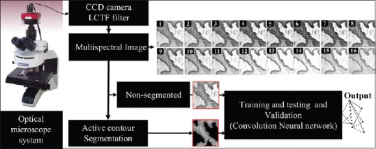
Flowchart of the proposed pipeline. Convolutional neural network classification of colorectal cancer tissues based on multispectral biopsy images

Data acquisition

Histological CRC data are obtained from anatomical pathology at the CHU Nancy Brabois Hospital. Part of these data was used in a previous study for classifying the abnormal PT from texture features.[9] Tissue samples were obtained from sequential colon resections of thirty patients with CRC. Sections of 5 μm thickness were extracted and stained using hematoxylin and eosin to reduce image processing requirements. Multispectral images of 512 × 512 pixels were then acquired using a CCD camera integrated with a LCTF in an optical microscopy system.[18] For each tissue sample, the LCTF was used to provide 16 multispectral images sampled uniformly across the wavelength range of 500–650 nm.[19] Since multispectral imaging considers a broader range of wavelengths, it can capture physiological characteristics of tissues beyond those provided by standard grayscale or trichromatic photography.

As mentioned before, the progression of CRC was modeled by considering three types of pathological tissues: BH, IN, and Ca. Each of the thirty biopsy samples used in this study was labeled by a senior histopathologist, for a total of ten BH samples, ten IN samples, and ten Ca samples.

Pathological tissue segmentation

Although unsegmented images can also be used directly, a segmentation step is added in the proposed pipeline to isolate the CRC tissues from nonrelevant tissues and structures such as lumen. For this step, we used a semi-automatic segmentation technique based on the active contour algorithm, which can accurately delineate the boundaries of irregularly shapes and has been shown to perform well for tissue segmentation.[20] Briefly, the active contour model can be described as a self-adaptive search for a minimal energy state E_AC, defined as the sum of an internal energyand an external energy E_ext.[21] The segmentation contour in an image I (x, y) is represented as a parametric function P (s) = (x (s), y (s)), s [0, 1] and is updated iteratively to minimize E_AC. The internal energy is defined as

Where p’ (s) and p’’ (s) represent the first and second derivatives of P (s), respectively, and α and β are constants weighting the relative importance of the derivatives. Intuitively, the internal energy favors short and smooth contour configurations. Likewise, the external energy is defined as:

Where G_σ (x, y) is the 2D Gaussian function with standard deviation σ and ∇ is the gradient operator. The external energy ensures agreement between the contour and image gradient information arising from tissue boundaries. Segmentation contours were initialized as centered rectangles of 508 × 508 pixels.

As shown in Figure 2, the segmentation algorithm partitions the image in two nonoverlapping regions, containing pixels that are on one side or the other of the segmentation contour. In a postprocessing step, a trained user (e.g., a pathologist) is asked to select the region of interest as one of the two segmented regions [Figure 2c]. Although outside the scope of this paper, a supervised learning model such as SVM could also be trained to select the region of interest automatically.

Figure 2.

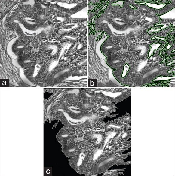
Example of tissue segmentation. (a) Original image, (b) segmentation obtained by the active contour model, (c) selected region of interest

To evaluate the performance of our segmentation model, we used manually annotated ground truth provided by the CHU Nancy-Brabois Hospital. The Jaccard similarity coefficient (JSC), dice similarity coefficient (DSC),[22,23] false positive rate (FPR),[24] and false negative rate (FNR)[25] were considered as performance metrics. The JSC and DSC metrics evaluate the degree of the correspondence between two segmentations (i.e., segmentation output and ground truth) and are defined as:

Where A and B represent the compared segmentations, TP/TNisthe number of correctly classified foreground/background pixels (i.e., true positives/negatives) and FP/FNisthe number of incorrectly labels foreground/background pixels (i.e., false positives/negatives). Moreover, FPR/FNR is the ratio between the number of pixels incorrectly labeled as foreground/background and the total number of background/foreground pixels:

We compared the performance of our active contour model with two standard segmentation approaches: Otsu's thresholding method[26] and edge detection.[27]

Convolutional neural network-based classification

As in most CNN-based classification approaches, we adopted an architecture consisting of three types of layers: convolution layers, subsampling (max-pooling) layers, and a fully-connected output layer.[28] These types of layer can be described as follows:

Convolution layer

This layer type receives as input either the image to classify or the output or the previous layer and applies a set of N_l convolution filters to this input. The output of the layer corresponds to N_l feature maps, each one the result of a convolution filter and some additive bias. The parameters learned during training correspond to the convolution filter and bias weights. Note that the convolution process trims output maps by a border of M_l − 1 pixels, where M_l × M_l is the size of convolution filters.

Subsampling (pooling) layer

This parameter-less type of layer reduces the size of input feature maps through subsampling, thereby supporting local spatial invariance. It divides the input maps into nonoverlapping subregions and applies a specific pooling function to each one of them. In our architecture, we considered the max-pooling strategy, which outputs the maximum value of each subregion. Note that the pooling process reduces the feature maps by a factor of M_l, where M_l × M_l is the size of pooling subregions.

Output (fully-connected) layer

This type of layer captures the relationship between the final layer feature maps and class labels. The output of the layer is a vector of K elements, each one representing the score of a class (e.g., K = 3 in our network). Fully-connected layers can be seen as convolution operations, in which filters have the same size as their input maps.

Figure 3 shows the proposed CNN architecture. This architecture is composed of two convolution layers (C₁ and C₃), each one followed by max-pooling layers (S₂ and S₄), and an output layer (F₆). Although not represented in the figure, a layer of Rectified Linear Units (ReLUs) is added after each max-pooling layer to improve the convergence of the learning process, which is based on the stochastic gradient descent algorithm. Further details on implementing CNNs may be obtained from.[28]

Figure 3.

Proposed convolutional neural network architecture with two convolution layers (C1 and C3), two max-pooling layers (S2 and S4), and one fully-connected layer (F5). For each layer, the filter size and number of output features are given

For training and evaluating the CNN, the data were split based on the patients. We randomly selected the data of 21 patients (7 BH, 7 IN and 7 Ca) for training and used the data of the remaining 9 patients (3 BH, 3 IN, and 3 Ca) for testing. Furthermore, the biopsy images of three training patients were held out in a validation set and used to determine the optimal network architecture and number of training epochs. For each patient in the training, validation, and testing sets, we obtained multiple examples by running a 60 × 60 × 16 sliding window across the original 512 × 512 × 16 multispectral images. These examples were given the same label as the original image and used as input to the CNN. For segmented images, only examples whose center is within the region of interest were kept. Thus, training examples obtained from segmented images contain more relevant information for the target classification problem. Accuracy, which corresponds to the percentage of correctly classified examples, was used as a measure of classification performance.

Results

In this section, we evaluate the performance of our CRC tissue classification method. Since this method uses segmentation as preprocessing step, we first assess the ability of the proposed segmentation algorithm to extract regions of interest corresponding to CRC tissues.

Table 1 gives the average performance of the three tested segmentation methods (Otsu's thresholding, edge detection, and active contour) on tissue samples corresponding to BH, IN, and Ca. We observe that our active contour method outperforms the other two approaches, for all performance metrics and tissue types (with P < 0.01 in a paired t-test). With respect to tissue types, the best performance of our method is obtained for Ca, with a JSC of 0.86, compared to 0.80 and 0.82 for BH and IN, respectively. Examples of segmentation results, for each tissue type, are shown in Figure 4. We see that the active contour method finds more consistent regions that better delineate the CRC tissues in the image.

Table 1.

Average performance obtained by three tissue segmentation methods on BH, IN and Ca tissue samples

Figure 4.

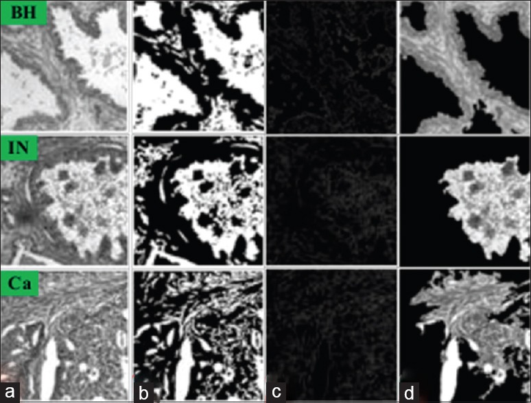
Examples of results obtained by the segmentation methods for the benign hyperplasia, intraepithelial neoplasia, and carcinoma tissue types. (a) Original image, (b) Otsu's thresholding, (c) edge detection, (d) active contour

Classification results are summarized in Table 2, showing the accuracy obtained on examples of the test set by our proposed CNN model, with and without the image segmentation step. For comparison, we also report accuracy values obtained by various tissue classification approaches on the same data. These approaches are categorized according to the type of texture or shape features used (e.g., gray-level co-occurrence matrix [GLCM], and statistical moments), classifier model (e.g., SVM and nearest-neighbors), and whether image segmentation is required or not. Note that these approaches work by quantifying a region (segmented or the whole image) with generic features and using these features as input to a classifier. In contrast, our proposed CNN method learns the features from training data, providing a better representation of the different CRC tissue types.

Table 2.

Comparison of tissue classification methods on the same data

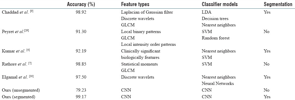
From these results, we observe that extracting regions of interest through segmentation enhances the accuracy of our method. Thus, while an accuracy of 79.23% is obtained without segmentation, the accuracy of our method reaches 99.17% on presegmented images. While this could be due to various other factors, extracting regions corresponding to CRC tissues provide more discriminative examples to train the CNN. In comparison to other tissue segmentation approaches, our CNN method with segmentation provides the highest accuracy (i.e., 99.17% vs. 98.92% for Chaddad et al.). Although relatively small, such improvement in accuracy can have a significant impact considering that the problem is cancer detection.

To illustrate the convergence of the parameter optimization phase (i.e., stochastic gradient optimization), Figure 5 shows the mean squared error (MSE) measured after each training epoch, corresponding to the mean squared difference between the network output Y_i’and target label vector Y_i:

Figure 5.

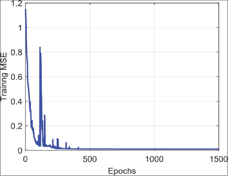
Variation of mean squared error across training epochs

We see that the optimization converges after 500 epochs and that the MSE upon convergence is nearly 0. This shows that the proposed architecture is complex enough to learn a discriminative representation of tissue types and that the learning rate is adequate. In practice, the best number of epochs is selected based on the validation accuracy.

However, eight segmented images were tested, and the performance metrics were increased with MSE and accuracy value of 0.0001 and 99.168%, respectively.

Discussion

The CRC tissue classification approaches presented in Table 2 are based on the assumption that such tissues can be effectively described using a generic texture or morphological features.[4,7,9,29,30] For example, Chaddad et al. used texture features derived from GLCMs, discrete wavelet transforms, and Laplacian of Gaussian filters, computed on presegmented regions, to classify the same images with an accuracy of 98.92%.[9] Likewise, Peyret et al. computed texture features such as local binary and local intensity order patterns, on unsegmented to images, obtaining an accuracy of 91.3%.[29] In contrast, we proposed a data-driven method, based on CNNs, to learn an optimal representation of tissues from training data. Our experiments showed this method outperforms existing approaches, even with a small number of tissue samples, with an accuracy of 99.17%. Results have also shown the usefulness of using presegmented images, which significantly improves the accuracy by focusing computation on relevant tissue regions within the image.

While results are promising, this study also has several limitations. First, it is based on a single small cohort of thirty patients. Having a larger set of biopsy images from different patients would help capture the full variability of tissues in the progression of CRC. Moreover, to obtain an optimal accuracy, our method currently requires the pathologist to select the region of interest from a segmented image. To have a fully automated pipeline, this step should be replaced by a supervised learning model which would determine the region of interest from training data.

Conclusions

We have presented a method for the classification of CRC tissues from multispectral biopsy images, based on active contour segmentation and CNNs. Unlike traditional approaches, which extract generic texture or shape features from the image, our method learns a discriminative representation directly from the data. Experiments on multispectral images of thirty patients show our method to outperform traditional approaches when using presegmented images. In future work, we will extend this study by including a larger number of patients and using a fully automated segmentation step.

Financial support and sponsorship

The University of Lorraine supports all the work of this research project.

Conflicts of interest

There are no conflicts of interest.

References

- 1.Roy T, Barman S. Performance analysis of network model to identify healthy and cancerous colon genes. IEEE J Biomed Health Inform. 2016;20:710–6. doi: 10.1109/JBHI.2015.2408366. [DOI] [PubMed] [Google Scholar]
- 2.Decker KM, Singh H. Reducing inequities in colorectal cancer screening in North America. J Carcinog. 2014;13:12. doi: 10.4103/1477-3163.144576. [DOI] [PMC free article] [PubMed] [Google Scholar]
- 3.Fu JJ, Yu YW, Lin HM, Chai JW, Chen CC. Feature extraction and pattern classification of colorectal polyps in colonoscopic imaging. Comput Med Imaging Graph. 2014;38:267–75. doi: 10.1016/j.compmedimag.2013.12.009. [DOI] [PubMed] [Google Scholar]
- 4.Kumar R, Srivastava R, Srivastava S. Detection and classification of cancer from microscopic biopsy images using clinically significant and biologically interpretable features. J Med Eng 2015. 2015:457906. doi: 10.1155/2015/457906. [DOI] [PMC free article] [PubMed] [Google Scholar]
- 5.Jass JR. Classification of colorectal cancer based on correlation of clinical, morphological and molecular features. Histopathology. 2007;50:113–30. doi: 10.1111/j.1365-2559.2006.02549.x. [DOI] [PubMed] [Google Scholar]
- 6.Rathore S, Hussain M, Khan A. Automated colon cancer detection using hybrid of novel geometric features and some traditional features. Comput Biol Med. 2015;65:279–96. doi: 10.1016/j.compbiomed.2015.03.004. [DOI] [PubMed] [Google Scholar]
- 7.Rathore S, Hussain M, Aksam Iftikhar M, Jalil A. Ensemble classification of colon biopsy images based on information rich hybrid features. Comput Biol Med. 2014;47:76–92. doi: 10.1016/j.compbiomed.2013.12.010. [DOI] [PubMed] [Google Scholar]
- 8.Rathore S, Iftikhar MA, Hussain M, Jalil A. Classification of colon biopsy images based on novel structural features. Emerging Technologies (ICET), 2013 IEEE 9th International Conference on: 2013, IEEE. 2013:1–6. [Google Scholar]
- 9.Chaddad A, Desrosiers C, Bouridane A, Toews M, Hassan L, Tanougast C. Multi texture analysis of colorectal cancer continuum using multispectral imagery. PLoS One. 2016;11:e0149893. doi: 10.1371/journal.pone.0149893. [DOI] [PMC free article] [PubMed] [Google Scholar]
- 10.Lawrence S, Giles CL, Tsoi AC, Back AD. Face recognition: A convolutional neural-network approach. IEEE Trans Neural Netw. 1997;8:98–113. doi: 10.1109/72.554195. [DOI] [PubMed] [Google Scholar]
- 11.Krizhevsky A, Sutskever I, Hinton GE. Imagenet classification with deep convolutional neural networks. Adv Neural Inf Process Syst. 2012;2012:1097–105. [Google Scholar]
- 12.Simard PY, Steinkraus D, Platt JC. Best practices for convolutional neural networks applied to visual document analysis. Seventh International Conference on Document Analysis and Recognition, 2003. Proceedings. 2003:958–63. [Google Scholar]
- 13.Stutz D. Understanding convolutional neural networks. InSeminar Report, Fakultät für Mathematik, Informatik und Naturwissenschaften Lehr-und Forschungsgebiet Informatik VIII Computer Vision. 2014 [Google Scholar]
- 14.Lo SB, Lou SA, Lin JS, Freedman MT, Chien MV, Mun SK. Artificial convolution neural network techniques and applications for lung nodule detection. IEEE Trans Med Imaging. 1995;14:711–8. doi: 10.1109/42.476112. [DOI] [PubMed] [Google Scholar]
- 15.LeCun Y, Bottou L, Bengio Y, Haffner P. Gradient-based learning applied to document recognition. Proc IEEE. 1998;86:2278–324. [Google Scholar]
- 16.Sahiner B, Chan HP, Petrick N, Wei D, Helvie MA, Adler DD, et al. Classification of mass and normal breast tissue: A convolution neural network classifier with spatial domain and texture images. IEEE Trans Med Imaging. 1996;15:598–610. doi: 10.1109/42.538937. [DOI] [PubMed] [Google Scholar]
- 17.Codella N, Cai J, Abedini M, Garnavi R, Halpern A, Smith JR. In: Deep Learning, Sparse Coding, and SVM for Melanoma Recognition in Dermoscopy Images. MLMI 2015. Zhou L, Wang L, Wang Q, Shi Y, editors. Switzerland: Springer; LNCS; 2015. pp. 118–26. [Google Scholar]
- 18.Chaddad A, Tanougast C, Dandache A, Bouridane A. Extracted Haralick's texture features and morphological parameters from segmented multispectrale texture bio-images for classification of colon cancer cells. WSEAS Trans Biol Biomed J. 2011;8:39–50. [Google Scholar]
- 19.Miller PJ, Hoyt CC. Photonics for Industrial Applications. Boston, MA: International Society for Optics and Photonics; 1995. Multispectral imaging with a liquid crystal tunable filter; pp. 354–65. [Google Scholar]
- 20.Pham DL, Xu C, Prince JL. Current methods in medical image segmentation. Annu Rev Biomed Eng. 2000;2:315–37. doi: 10.1146/annurev.bioeng.2.1.315. [DOI] [PubMed] [Google Scholar]
- 21.Kass M, Witkin A, Terzopoulos D. Snakes: Active contour models. Int J Comput Vis. 1988;1:321–31. [Google Scholar]
- 22.Guerard A. The serum diagnosis of typhoid fever. J Am Med Assoc. 1897;29:10–5. [Google Scholar]
- 23.Haj-Hassan H, Chaddad A, Tanougast C, Harkouss Y. Segmentation of abnormal cells by using level set model. Control, Decision and Information Technologies (CoDIT), 2014 International Conference on: 2014, IEEE. 2014:770–3. [Google Scholar]
- 24.Burke DS, Brundage JF, Redfield RR, Damato JJ, Schable CA, Putman P, et al. Measurement of the false positive rate in a screening program for human immunodeficiency virus infections. N Engl J Med. 1988;319:961–4. doi: 10.1056/NEJM198810133191501. [DOI] [PubMed] [Google Scholar]
- 25.Walter SD. False Negative Rate. Encyclopedia of Biostatistics. John Wiley & Sons, Ltd; 2005. [Google Scholar]
- 26.Otsu N. A threshold selection method from gray-level histograms. IEEE Trans Syst Man Cybern. 1979;1:62–6. [Google Scholar]
- 27.Senthilkumaran N, Rajesh R. Edge detection techniques for image segmentation – A survey of soft computing approaches. Int J Recent Trends Eng. 2009;1:250–4. [Google Scholar]
- 28.Phung SL, Bouzerdoum A. Matlab library for convolutional neural networks. ICT Research Institute, Visual and Audio Signal Processing Laboratory, University of Wollongong, Tech. Rep. 2009 [Google Scholar]
- 29.Peyret R, Bouridane A, Al-Maadeed SA, Kunhoth S, Khelifi F. Texture analysis for colorectal tumour biopsies using multispectral imagery. Engineering in Medicine and Biology Society (EMBC); 2015, 37th Annual International Conference of the IEEE, 2015: IEEE. 2015:7218–21. doi: 10.1109/EMBC.2015.7320057. [DOI] [PubMed] [Google Scholar]
- 30.Elgamal M. Automatic skin cancer images classification. Int J Adv Comput Sci Appl. 2013;4:287–94. [Google Scholar]