The effect of beam purity and scanner complexity on proton CT accuracy

Abstract

Purpose

To determine the dependence of the accuracy in reconstruction of relative stopping power (RSP) with proton computerized tomography (pCT) scans on the purity of the proton beam and the technological complexity of the pCT scanner using standard phantoms and a digital representation of a pediatric patient.

Methods

The Monte Carlo method was applied to simulate the pCT scanner, using both a pure proton beam (uniform 200 MeV mono‐energetic, parallel beam) and the Northwestern Medicine Chicago Proton Center (NMCPC) clinical beam in uniform scanning mode. The accuracy of the simulation was validated with measurements performed at NMCPC including reconstructed RSP images obtained with a preclinical prototype pCT scanner. The pCT scanner energy detector was then simulated in three configurations of increasing complexity: an ideal totally absorbing detector, a single stage detector and a multi‐stage detector. A set of 15 cm diameter water cylinders containing either water alone or inserts of different material, size, and position were simulated at 90 projection angles (4° steps) for the pure and clinical proton beams and the three pCT configurations. A pCT image of the head of a detailed digital pediatric phantom was also reconstructed from the simulated pCT scan with the prototype detector.

Results

The RSP error increased for all configurations for insert sizes under 7.5 mm in radius, with a sharp increase below 5 mm in radius, attributed to a limit in spatial resolution. The highest accuracy achievable using the current pCT calibration step phantom and reconstruction algorithm, calculated for the ideal case of a pure beam with totally absorbing energy detector, was 1.3% error in RSP for inserts of 5 mm radius or more, 0.7 mm in range for the 2.5 mm radius inserts, or better. When the highest complexity of the scanner geometry was introduced, some artifacts arose in the reconstructed images, particularly in the center of the phantom. Replacing the step phantom used for calibration with a wedge phantom led to RSP accuracy close to the ideal case, with no significant dependence of RSP error on insert location or material. The accuracy with the multi‐stage detector and NMCPC beam for the cylindrical phantoms was 2.2% in RSP error for inserts of 5 mm radius or more, 0.7 mm in range for the 2.5 mm radius inserts, or better. The pCT scan of the pediatric phantom resulted in mean RSP values within 1.3% of the reference RSP, with a range error under 1 mm, except in exceptional situations of parallel incidence on a boundary between low and high density.

Conclusions

The pCT imaging technique proved to be a precise and accurate imaging tool, rivaling the current x‐rays based techniques, with the advantage of being directly sensitive to proton stopping power rather than photon interaction coefficients. Measured and simulated pCT images were obtained from a wobbled proton beam for the first time. Since the in‐silico results are expected to accurately represent the prototype pCT, upcoming measurements using the wedge phantom for calibration are expected to show similar accuracy in the reconstructed RSP.

1. Introduction

Proton computerized tomography (pCT) is a relatively new imaging technology capable of reconstructing the 3D map of the relative stopping power (RSP); that is, the proton stopping power in the patient relative to that in water. The RSP can be imported into a proton treatment planning system for dose calculation or used to verify patient positioning and the treatment plan. In existing proton treatment centers, dose calculations are currently performed using Hounsfield units from an x‐ray computed tomography (CT) scan that are then converted to RSP. The use of x‐ray CT images ignores fundamental differences in physical interaction processes between photons and protons and is, therefore, potentially inaccurate.^{1, 2} Dual energy CT (DECT), is under investigation to improve the accuracy of the RSP determination in the patient.^{3, 4, 5} On the other hand, as shown in the first pCT studies from 40 years ago,^{6, 7, 8} pCT images are directly impacted by proton processes and also have a dose advantage compared to x‐ray CT. In 2008, a collaboration including Loma Linda University (LLU), University of California Santa Cruz (UCSC) and Northern Illinois University (NIU) started the development of a prototype Phase I pCT scanner capable of imaging a small phantom head. The Phase I scanner consisted of four position‐sensitive detector modules to infer proton path and a segmented CsI (Tl) crystal calorimeter as a residual energy‐range detector (RERD). With this scanner and earlier conceptual studies using Monte Carlo simulations encouraging results were reported, indicating that an RSP accuracy of better than 1% may be possible.^{9, 10, 11, 12, 13, 14, 15, 16, 17, 18, 19} In 2011, LLU, UCSC, and California State University, San Bernardino (CSUSB), started the development of the next generation phase II pCT scanner. The system, completed in 2011, is capable of imaging phantom heads and QA phantoms with protons of a nominal energy of 200 MeV. The device dimensions and the position‐sensitive detector modules are similar in essential characteristics to the first generation system, with the exception of a larger sensitive tracking area (9 cm × 36 cm instead of 9 cm × 18 cm) and replacement of the original RERD by a multi‐stage scintillator (MSS), consisting of a stack of five fast plastic scintillators, read out by photomultiplier tubes.^{20, 21, 22} This design provides a more accurate determination of the residual energy/range of protons, compared with the calorimeter of the first generation system.²³ The pCT collaboration also developed a novel calibration procedure, to convert the response of the RERD directly to water‐equivalent path length (WEPL), and provided effective algebraic reconstruction algorithms for the reconstruction of RSP images.^{24, 25}

In addition to statistical uncertainties, resulting from noise in the acquired pCT data, systematic uncertainties in the RSP reconstruction can arise during the steps of pCT data acquisition and subsequent image reconstruction and from the assumption of a mono‐energetic proton beam. The sources of systematic uncertainties and their relative importance have not been well determined. The goal of the present work was to use the Monte Carlo method to determine the dependence of these systematic uncertainties on the purity of the proton beam and the complexity of the pCT scanner and its calibration. Simulation beam purity ranged from a broad, normally incident mono‐energetic beam and a totally absorbing detector to a detailed simulation of the phase II pCT scanner installed downstream of the treatment head operated in uniform scanning mode at the Northwestern Medicine Chicago Proton Center (NMCPC), Warrenville, IL, USA, where the scanner has been studied since May 2015. The simulations were performed using the TOPAS (TOol for PArticle Simulation, TOPAS MC Inc., Oakland, CA, USA, http://www.topasmc.org) platform,²⁶ which is based on the Geant4 toolkit.^{27, 28} The geometry of the pCT scanner was implemented in Geant4 and validated with respect to a different beam line.²⁹

In this study, the implementation of the NMCPC beam line and the pCT scanner in TOPAS was first validated with measurements acquired at NMCPC, for the first time acquiring and simulating pCT images using a wobbled beam. The TOPAS tool was then used to investigate the sources of systematic uncertainty introduced during the steps leading to RSP reconstruction for standard phantoms and a digital representation of a pediatric patient whose stopping power values were accurately known. The study started with an ideal setup, in order to reduce sources of systematic uncertainty, then a realistic proton beam and increasing complexity in the energy detector were added to evaluate their contribution to the accuracy of the reconstructed RSP values.

2. Theory

In a pCT scan, the energy loss of individual protons crossing an object (such as a patient) from different directions is measured and used to reconstruct a 3D image of the RSP of the object. Protons lose energy through the object and exit with an energy that is reduced by ΔE. The RSP for each voxel traversed is related to the exiting energy and the WEPL:

$$\underset{L}{\overset{}{\int }}RSP\left(l\right)dl=\underset{E_{in}}{\overset{E_{out}}{\int }}\frac{dE}{S_w}=WEPL,$$ (1)

where the exiting energy $E_{out}=E_{in}-\mathrm{\Delta }E$, S _w is the stopping power for protons in water, WEPL is the water‐equivalent path length for each track through the object, L is the proton path through the object, and E _in is the incident energy of the proton beam, typically around 200 MeV. RSP(l) is the ratio of the proton stopping power S at the distance l on the path L to that of water at the same proton energy E:

$$RSP\left(l\right)=\frac{S\left(E\left(l\right)\right)}{S_w\left(E\left(l\right)\right)}$$ (2)

The integral in Eq. (1) can be approximated by a discreet sum of RSPs times the length of the most likely path (MLP) for each voxel crossed by the track. This sum is the WEPL for that track. Writing this linear equation for each track leads to a system of linear equations that can be used to solve for the RSP for each of the voxels. In matrix formalism:

$$A\overrightarrow{x}=\overrightarrow{b}$$ (3)

where $\overrightarrow{b}$ represents the n dimensional vector of WEPL for n protons through the anatomical region of interest and $\overrightarrow{x}$ is an m dimensional vector corresponding to the RSP for each of the m voxels in the region of interest. The elements a _ij in the matrix A correspond to the MLP length (chord length) of the i‐th proton through the j‐th voxel. Since only a few hundred voxels are crossed by any given proton track, the elements of matrix A will be mostly 0s, and hence, a sparse large matrix (e.g., 10⁷ columns representing the incident proton positions and directions by 10⁹ rows representing the voxels in the object for an adult head size phantom).

The tracker system of the pCT device is used to measure the entrance and exit position and direction of each single track, while the RERD is used to measure the exiting energy to determine the WEPL for each track. The entrance and exit trajectories allow constructing the MLP of each proton through the patient and hence the chord length (a _ij ) through each voxel.¹⁵ The RSP image reconstruction problem is then reduced to solve the large linear system in Eq. (3).

3. Materials and methods

3.A. Simulation method and experimental validation

TOPAS release 2.0 with Geant4 version 9.6 patch 4 was used to produce the simulated data shown in this work. The physics list activated considers both electromagnetic and nuclear process; it has been comprehensively validated and details about it are published elsewhere.³⁰

The pCT phase II scanner (Fig. 1) was composed of a tracker system, used as a position‐sensitive detector, and MSS used as RERD. The tracker system consisted of 4 tracker planes (P0–P3), 2 positioned upstream (the front trackers P0 and P1) and 2 downstream (the rear trackers P2 and P3) of the isocenter. The tracker system was symmetric with respect to the isocenter. The most inner planes (P1 and P2) were at a distance of 164.3 mm from the isocenter, while the most outer (P0 and P3) at 214.35 mm. Each plane was made of 2 silicon boards, 349 × 86 × 0.4 mm³, each of them used to score the position of the tracked protons.^{21, 22} The MSS aperture was 37.5 × 10 cm², designed to optimize the accuracy of the WEPL measurements while simplifying the detector construction and the performance requirements of its components. Each of the 5 stages was a 5.08 cm thick block of polystyrene (1.06 g/cm³). The average WEPL measurement accuracy is about 3.0 mm per proton in the 0 to 260 mm WEPL range required for a pCT head scan with a 200 MeV proton.²³

Figure 1.

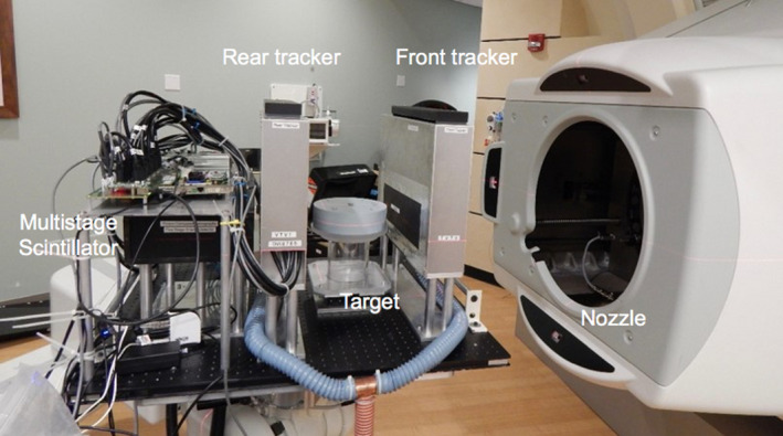
The pCT phase II scanner set up at the NMCPC.

The NMCPC beam line was commissioned using measured beam lateral profiles for three field sizes and three different configurations of scatterers and Bragg curves covering the full energy range of 100–225 MeV. Bragg curves were measured in water with a PTW Bragg peak parallel plate ionization chamber with an effective diameter of 8.4 cm. Lateral profiles were measured in air with a MatriXX (IBA Dosimetry) detector, an array of 1020 ionization chambers evenly distributed in a rectilinear grid over an active area of 24.4 × 24.4 cm². Beam energy was determined from the measured beam penetration, energy spread from the measured width of the Bragg peak, and spot size of the source from the measured spot size in air at isocenter. The initial spot size was adjusted to reproduce experimental un‐wobbled spots profiles in air for 200 MeV beams using three geometrical configurations of scatterers including: (a) No scatterers, (b) Scatter 4 only (lead foil of 1 mm thickness) and (c) combined Scatters 1, 7, and 8 (Lexan stack of foils of 9.59 mm combined thickness). The same spot size was used for all energies, although only 200 MeV is used in the pCT simulations. The simulation of the treatment head was dynamic as it included the steering (wobbling) of the beam by means of magnetic fields. In TOPAS a magnetic field can be attached to any component or volume. Dipole magnetic fields were used in the first and second magnet of the treatment head with field directions pointing to the y‐axis and x‐axis, respectively. The magnetic field strength was determined from a fit of the measured and simulated field sizes.

The simulation of the pCT scanner in the NMCPC beam line (Fig. 2) was validated using the measured reconstructed RSP distribution from a scan of a water cylinder. In this case the phantom was an 8 cm radius, 8 cm thick water cylinder, clad in 2 cm thick, 1.18 g/cm³ acrylic. The measurement was conducted with the 200 MeV wobbled beam with beam current sufficiently low to track single protons. The raw data preprocessing allowed detection and dumping events where more than one proton was detected. Experimental effects such as noise and synchronization that were not simulated were evaluated for their affect on RSP determination by comparing the measured and simulated pCT images. Both were calibrated with the step phantom, and were for the same beam and detector configuration.

Figure 2.

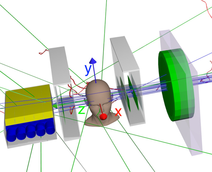
The phase II pCT scanner in the NMCPC beam line, as implemented in the TOPAS simulation. The (x, y, z) beam coordinates are shown. In the experiment the head was rotated around the y‐axis with the beam stationary.

3.B. Simulated energy detector and proton beam configurations

The pCT energy detector was simulated with three configurations (A–C) with different degrees of complexity as follows:

• No energy detector was simulated. The proton kinetic energy was scored directly on the tracker planes and the proton energy loss calculated as the difference between the energy on the P1 and P2 planes. This is equivalent to a totally absorbing detector.

• Single stage plastic energy detector (10 × 37.5 × 25.4 cm³) was used.

• A 5‐stage scintillator, reproducing the MSS of the pCT phase II scanner, was used as described above.

All phantoms and energy detectors were simulated using both a 9 × 36 cm² flat 200 MeV proton beam and the 200 MeV wobbled NMCPC proton beam. For the energy detector response, only the energy deposited in the sensitive volumes of the detector was scored.

3.C. Simulated WEPL calibration

The WEPL calibration curves for configuration A and B were calculated by simulating a special polystyrene step phantom (Fig. 3) developed to speed up and simplify the experimental pCT scanner calibration procedure. It contains three pyramids along the x‐axis direction with 6.35 mm steps, providing step‐wise variation of polystyrene thickness from 0 to 50.8 mm in the beam direction. To cover the full range of WEPL that can be imaged with 200 MeV protons, four removable polystyrene bricks of 50.8 mm thickness are successively added to the variable part of the phantom during the calibration. The maximum physical and water‐equivalent polystyrene thickness traversed by protons is thus, respectively, 254 mm and 263.7 mm, allowing the calibration of the detector over this WEPL range.²³ The polystyrene bricks and steps were made from a polystyrene block of Rexolite^® (C‐Lec Plastics, Inc. 6800 New State Road Philadelphia, PA 19135, USA http://www.rexolite.com/) consisting of CAS #9003‐53‐6 ([CH₂CH(C₆H₅)]_n) with density of 1.05 g/cm³ (manufacturer specification). The measured density was 1.046 ± 0.003 g/cm³, in agreement with the manufacturer specification. The water‐equivalent thickness of the bricks (up to 3 bricks) was determined from 200 MeV proton depth dose curves measured in water for both spread out Bragg peak and a pristine Bragg peak (R80 and R90). Averaged over all measurements, the RSP was found to be 1.030 ± 0.003, density being the main source of uncertainty. The lateral scatter effect was not considered in the RSP evaluation, but was accounted for in the calibration procedure, where the path length through polystyrene was calculated using the proton entrance and exit point coordinates coupled with Monte Carlo simulation. The WET values were obtained using polystyrene RSP = 1.038, evaluated for Geant4 polystyrene using the National Institute of Standards and Technology (NIST) data (density 1.06 g/cm³ corresponding to the NIST Pstar range tables).

Figure 3.

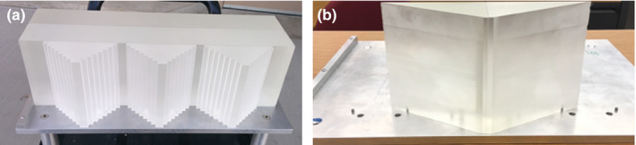
The two calibration phantoms: (a) step phantom (used with all the configurations) and (b) wedge phantom (used with configuration C only).

The simulated calibration procedure was performed in five separate runs. In the first run, data were collected just for the stairs parts of the step phantom, while in the following four runs the four bricks were added in sequence. In this way, 41 known WEPL step‐lengths were accounted for. Using the tracking information, the geometrical path lengths in polystyrene and air traversed for each proton history were reconstructed. Each WEPL value was evaluated as the sum of air and polystyrene path lengths multiplied by their corresponding relative stopping powers. These values were binned in 41 calibration points corresponding to the different thicknesses of polystyrene in 6.35 mm steps. For the energy detector configurations A and B the WEPL calibration curves were obtained by plotting, the average residual energy versus the WEPL step‐length per each step. The residual energy was evaluated for configuration A and B, respectively, as the difference between the initial energy and energy loss in the phantom, and the energy deposited in the single stage plastic energy detector. Each calibration point, thus corresponded to the mean value of the energy distribution (well approximated by a Gaussian) associated to a certain WEPL value. The full set of points was then interpolated by a 2nd and 4th degree polynomial curve. Although both curves fit the points well, the 4th degree fit was chosen for the energy to WEPL calibration curve because of the better accuracy obtained. For example, in configuration A the accuracy was 2.08 mm for the 4th degree versus 2.11 mm for the 2nd degree. The step phantom and the four bricks allowed studying the WEPL dependency on the energy all along the penetration depth of Bragg curve. In fact, when few steps were crossed, the plateau region was considered, while when the maximum thickness was crossed, the Bragg peak region was considered.

For configuration C, the WEPL calibration was performed using two different methods. The first method used the same step phantom as for configurations A and B. For each calibration point (each step in the phantom), the average energy deposited in the stage in which the proton stopped was evaluated. The dependence of the energy deposited in each stage of the MSS on the geometrical calculated WEPL was approximated by quadratic interpolation and a set of interpolation coefficients was stored. A similar method was used for calibration of the measurement.

With the first calibration method, relatively large ring reconstruction artifacts were seen, particularly in the reconstruction of the water phantom. Since these artifacts, were absent with the less complex energy detector configurations, it became clear that they were related to mis‐representation of the WEPL of protons stopping near the interface between the stages. To address this problem, a second, more recently developed method was implemented that used two polystyrene wedges (Fig. 3) instead of the stairs of the step phantom, providing a smooth variation in polystyrene thickness between 0 to 50.8 mm. Again, the calibration procedure was performed in five runs with polystyrene bricks added consecutively to cover the full range of WEPL, which was reconstructed using tracking information. In contrast to the step‐phantom calibration approach producing 41 discrete WEPL‐energy pairs as described above, this method yielded continuous WEPL‐energy distributions that were stored as 260 × 340 (columns × rows) tables for WEPL and energy in the corresponding 0–260 mm and 0–85 MeV ranges (i.e., in 1 mm and 0.25 MeV bins) for each detector stage where the proton stopped. The table WEPL rows were used to calculate WEPL peak position as an arithmetic mean over a full‐width half‐maximum window (asymmetric in the general case). The resulting 340 element vector represented the WEPL versus stage energy calibration curve for the corresponding stage.

The calibration curves were then used in the preprocessing of data obtained from scanning and object, to convert the residual energy for each single‐proton history into WEPL.

3.D. pCT image reconstruction

For both the simulated and the experimental scans 90 projection at 4° steps were used. The image reconstruction method adopted by the pCT collaboration uses the MLP concept for an iterative reconstruction algorithm, which allows extrapolating the curved proton path to produce tomographic reconstructions with sufficient spatial resolution and to minimize the effect of multiple Coulomb scattering. Several authors have modeled the multiple Coulomb scattering effects on proton path while crossing uniform material.^{31, 32, 33, 34} The compact, matrix‐based MLP formalism chosen by the pCT collaboration used a scattering model similar to the one described by Williams³⁵ but employed Bayesian statistics to determine the lateral displacement and direction of maximum likelihood at any intermediate depth within a uniform absorbing material.¹⁵ Before starting the iterative process, a fast reconstruction based on filtered back projection was used to determine the outer contour of the object in the reconstruction space and to provide entry and exit points for the MLP calculation. Moreover, the filtered back projection values give the initial estimate of the RSP in Eq. (3). The total number of n proton histories traversing the object was collected and the MLP of each history calculated from tracker information (entry point and direction and exit point and direction) and used to fill the n × m matrix A, where m is the number of voxels in 3D reconstruction space. The vector $\overrightarrow{b}$ contains the WEPL values obtained using the calibration procedure described above. The large linear system in Eq. (3) was solved using a fast, parallelizable iterative project algorithm combined with superiorization methods. To make the reconstruction process faster, the reconstruction program was implemented to run on both central process units and graphics processing units. ^{24, 25}Both the simulated and the experimental pCT images were reconstructed with a slice thickness of 1.25 mm, using 6 iterations with the FBP image as the initial iterate, 40 blocks, and a relaxation parameter of 0.1 for the block iterative reconstruction algorithm. Using these settings, and running the reconstruction on a Intel^® Xeon^® (Intel Corporation, Santa Clara, CA, USA) E5645 @ 2.40GHz CPU equipped with an NVIDIA (Santa Clara, CA, USA) GeForce GTX 780 GPU, the reconstruction took about 30 minutes.

3.E. Estimation of RSP reference values

For the evaluation of the pCT reconstructed RSP accuracy, the RSP used in TOPAS was determined to serve as reference values to evaluate the accuracy of the RSP values reconstructed from the simulated pCT data. The composition of each material in the simulation was taken from the data sheets of the CIRS (Computerized Imaging Reference Systems, Inc., Norfolk, VA, USA) phantom project 11‐575 (model 715 customized), with the percentages by weight of those elements with the highest percentages adjusted slightly to force the sum of all weights to be exactly 100%, a requirement of TOPAS (Table 1). The effect on the RSP value was not larger than 0.1%.

Table 1.

Material composition showing percentages by weight. When two percentages are given, the first is the value from the manufacturer, the second the value used in the simulation adjusted so that the sum of the percentages is exactly 100%. For trabecular bone and tooth enamel, no modification was necessary. Reference RSP values were calculated using TOPAS. Water was simulated as G4_Water; that is, H₂O with I = 78 eV, with a density of 1 g/cm³

Material	Element (percentage by weight)	Density (g/cm3)	Reference RSP
Soft tissue (gray)41	C (57.44, 57.45), O (24.59, 24.60), H (8.47, 8.48), N (1.65), Mg (7.62), Cl (0.19)	1.055	1.042
Brain tissue (average)42	C (53.60, 53.62), O (26.49, 26.51), H (8.16, 8.17), N (1.53), Mg (9.98), Cl (0.19)	1.070	1.052
Spinal cord42	C (54.27, 54.28), O (26.59, 26.60), H (7.36), N (2.17), Mg (9.37), Cl (0.22)	1.070	1.040
Spinal disk Pediatric	C (52.45, 52.46), O (27.60), H (7.09), N (2.11), Ca (0.98), Mg (9.55), Cl (0.21)	1.100	1.064
Trabecular bone Pediatric	C (59.65), O (21.42), H (8.39), N (1.55), Ca (5.03), Mg (1.46), Cl (0.12)	1.130	1.114
Tooth dentine	C (35.35, 35.36), O (29.41), H (4.51), N (1.23), Ca (19.48), Cl (0.04)	1.660	1.515
Cortical bone 5 year old43	C (29.69, 29.70), O (34.11, 34.12) H (4.13), N (0.85), Ca (20.48), Mg (3.11), Cl (0.04)	1.750	1.586
Tooth enamel	C (21.81), O (34.02), H (2.77), N (0.82), Ca (26.60), Cl (0.03)	2.040	1.786

For each material in (Table 1), the mean proton stopping power was calculated for protons with initial kinetic energy over the energy range from E ₀ = 100 MeV to E _f = 200 MeV (not including the Bragg peak) with 1000 equal energy steps, without tracking the particles, with the following equation:³⁶

$$\overline{S_m}=\frac{{\int }_{E_0}^{E_f}{S}_m\left(E\right)dE}{{\int }_{E_0}^{E_f}dE}$$ (4)

where S _m is the restricted stopping power calculated with the Geant4's Bethe‐Bloch equation via the GetDEDX method in the G4EmCalculator class using a high (effectively infinite) production cut. The RSP of each material was then calculated by dividing the evaluated Eq. (4) for each material to the corresponding value for water with a ionization potential I = 78 eV.

3.F. Simulated phantoms

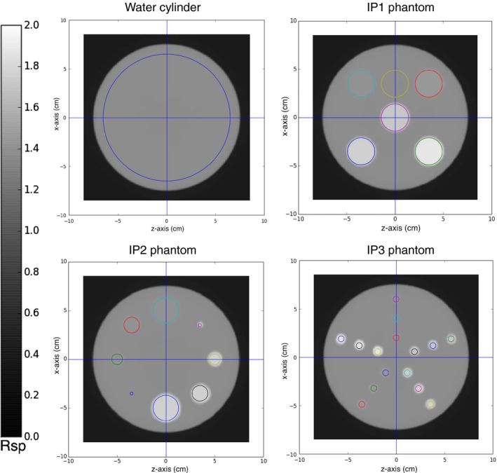
The following phantoms (Fig. 4) were simulated to investigate the accuracy of the reconstructed RSP as a function of the insert material, the insert dimension, and its radial position:

• Water cylinder 15 cm diameter, 8 cm thick

• Insert Phantom 1 (IP1): same water cylinder with five inserts (each insert 8 cm thick, 1.5 cm radius) made of different materials; one insert was placed at the phantom center while the other four are placed 5 cm from the phantom center.

• Insert Phantom 2 (IP2): same phantom body as IP1, but with two types of 8 cm thick material inserts and different dimensions placed with their centers 5 cm from the center of the phantom.

• Insert Phantom 3 (IP3): same water cylinder with 8 cm thick, 0.5 cm radius inserts placed at different distances from the phantom center.

Figure 4.

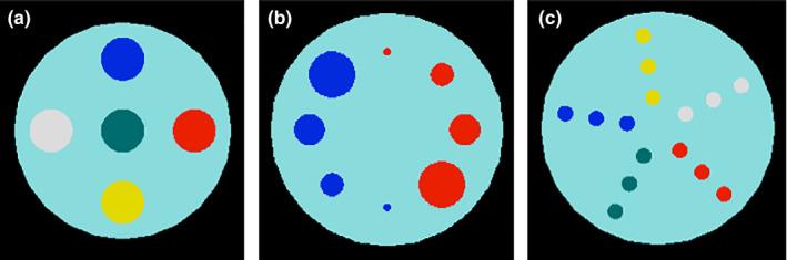
The simulated water phantoms containing different kinds of inserts. (a) IP1: water phantom with inserts of tooth enamel (white), cortical bone (blue), brain tissue (red), trabecular bone (yellow), and tooth dentine (green). (b) IP2: water phantom with inserts of brain tissue (red) and cortical bone (blue) with different radii: 1.5 cm, 1.0 cm, 0.75 cm, and 0.25 cm. (c) IP3: water phantom with 0.5 cm radius inserts at different radial positions (2 cm, 4 cm, 6 cm from the center) for 5 different materials using the same color scheme as in (a).

In addition, a digital head and trunk phantom of a 10‐year old human female was simulated.³⁷ The phantom consisted of 193 × 153 × 822 cubic voxels of 2 mm width. Each voxel was assigned a specific material composition and density, according to ICRP report 110.³⁸ The RSP distribution was calculated over the energy range from E ₀ = 100 MeV to E _f = 200 MeV as previously described. The calculated values were used as a reference to compare to the results of the simulated pCT image reconstruction. To fit the phantom in the pCT scanner in the simulation, only the head was scanned, with the phantom dimensions cut to 90 × 114 × 103 voxels.

The set of simulations done for the different energy detector configurations, beams, and phantoms is listed in Table 2.

Table 2.

Summary of the different simulation setups (see Materials and Methods section). The ideal beam was a 200 MeV mono‐energetic, 9 × 36 cm², parallel proton beam. The realistic beam was the clinical beam used for uniform scanning at NMCPC, modeled with TOPAS

Configuration	A	B	C
Energy detector	Totally absorbing	Single stage	MSS (5 stages)
Beam	Ideal	Ideal	Ideal and realistic
Calibration	Step	Step	Step and wedge
Phantoms	Water	Water	Water
	IP1	IP1	IP1
	IP2	IP2	IP2
	IP3	IP3	IP3
			Human head

4. Results

4.A. Validation of the simulation of the NMCPC beam line

Beam lateral profiles measured in air at isocenter are shown in Fig. 5 compared to simulated results for a range of wobbling magnet currents. The measured beam widths from the profiles (full‐width half‐maximum) were in general 0.8 ± 0.3 mm wider on the x‐axis and 0.9 ± 0.2 mm wider on the y‐axis than the simulated result (1 standard deviation).

Figure 5.

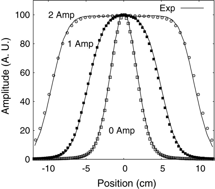
Comparisons between the TOPAS simulation of the NMCPC beam line and experimental data for 200 MeV protons showing lateral profiles at different scanning magnet current amplitudes. TOPAS data are shown as symbols. Experimental data are shown as solid lines.

The measured Bragg curves for 98–228 MeV proton beams are shown in Fig. 6. The range and peak width σ were obtained from measured and simulated Bragg curves covering the full range of energies available on this beam line by fitting each curve to an analytical expression by Bortfeld.³⁹ Results of the comparison to simulation (Fig. 6) show the maximum difference in σ was 0.16 mm and the maximum difference in range was 0.5 mm. The peak to plateau ratio was reliably available from measurement from 113 MeV up to the maximum energy of 228 MeV. The simulation agreed with measurement over this energy range within 2% for energies below 211 MeV and 4% above this energy. The nuclear model used in the simulations (Geant4 Binary nuclear model QGSP_BIC_HP) describing the production of secondary particles at the plateau region can explain the larger discrepancy at higher energies.

Figure 6.

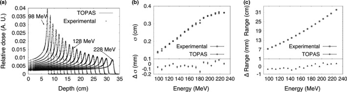
(a) Bragg curves, (b) Bragg peak σ, and (c) proton range at 80% of the maximum dose on the distal side of the Bragg peak for 98–228 MeV proton beams in water. The difference in the measured and calculated results is shown for σ and range. Error bars represent one standard deviation of the combined statistical and fitting uncertainty for TOPAS and the fitting uncertainty for the experimental data.

4.B. Calculation of reference RSP values

Reference RSP values calculated for the materials placed in the water cylinder for simulation of pCT scans are listed in Table 1. The reference RSP distribution was also calculated for the digitized pediatric phantom using ICRP 110 materials, with the value of the water ionization potential set to 78 eV. A sagittal slice through the head is shown in Fig. 7.

Figure 7.

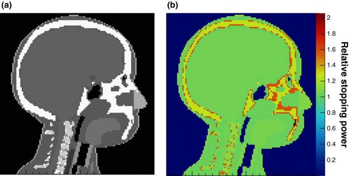
(a) Sagittal slice through the head of the digital phantom with a different gray scale for each medium (left, denser media are lighter). (b) Reference RSP, calculated with Eq. (4). The color bar displays the corresponding RSP values.

4.C. Configuration A: ideal beam with totally absorbing energy detector

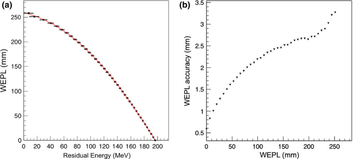
The WEPL calibration curve for configuration A obtained from simulation of the step phantom is shown in Fig. 8(a). The WEPL uncertainties are plotted in Fig. 8(b) for each of the 41 WEPL step lengths. The average WEPL error was 2.08 mm.

Figure 8.

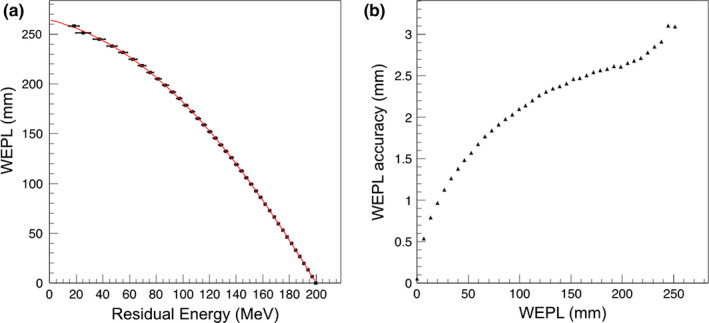
(a) The WEPL calibration curve (black points fit to red curve) obtained in configuration A, using the polystyrene step phantom and a mono‐energetic rectangular proton source. The error bar corresponds to the standard deviation of the energy distribution at each point. (b) Average single‐proton WEPL uncertainty for this configuration.

The central transverse slice through the reconstructed water phantom images of the 4 phantoms for configuration A is shown in Fig. 9. The average RSP value for the reconstructed water was 1.002 ± 0.1%, within 0.2% of the expected value of unity. The uncertainty was estimated as the standard deviation of the reconstructed RSP distribution in the area of interest [blue circle in Fig. 9(a)]. The lateral profile through the central slice of the reconstructed water image is shown in Fig. 10. The maximum discrepancy from the average value for configuration A is 0.28%. The results for the IP1, IP2 and IP3 phantoms are shown in Figs. 11, 12, 13. The RSP values reported correspond to the mean RSP values in a region of interest (ROI, as indicated by the colored circles in Fig. 9) for ten consecutive slices, with its relative standard deviation. For the water phantom the ROI had a radius of 60 mm. For IP1 and IP3 phantoms, respectively, the ROIs for inserts have radii of 13 mm and 3 mm. For the IP2 phantom the ROIs had radii of 1.5 mm, 5.5 mm, 8 mm, 13 mm from the smallest to the biggest, respectively. These radii, slightly smaller than the inserts’ radii, were chosen to avoid the outer region of the inserts, where the loss of spatial resolution due to Multiple Coulomb scattering would cause systematic RSP error. The mean, minimum and maximum error for all inserts for each one of the IP1, IP2, and IP3 phantoms are reported in Table 3.

Figure 9.

Transverse slice through the pCT reconstructed RSP image of the water cylinder and the phantoms IP1, IP2, and IP3 for configuration A (ideal 200 MeV beam, totally absorbing energy detector). The reconstructed images have a slice thickness of 1.25 mm with 256 × 256 pixels in an evenly spaced grid with 0.66 mm spacing. The colored circles indicate the regions of interest where the RSP was measured for each insert. The RSP was calculated in the ROIs over ten consecutive transverse slices, from five slices below the central slice (shown in figure) to four slices above.

Figure 10.

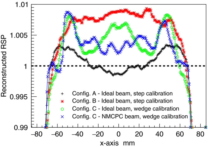
Comparison of the RSP lateral profiles for the water phantom for all configurations investigated. The expected RSP is unity.

Figure 11.

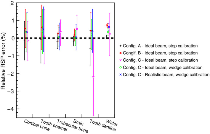
Comparison of RSP values reconstructed for the IP1 phantom in different configurations. The RSP relative error is calculated as the difference between reconstructed and reference values, divided by the reference value. The error bars represent the percentage relative standard deviations in each region of interest (see Fig. 9).

Figure 12.

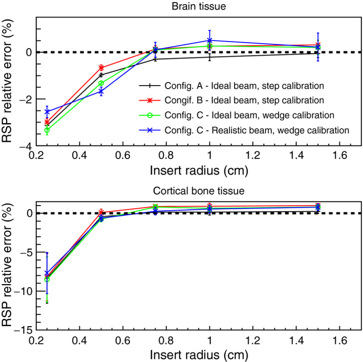
Comparison of RSP values versus insert radius dimension, reconstructed for the IP2 phantom and the 0.5 cm radius cylinders in the IP3 phantom (linearly interpolated to 5 cm from the center of the phantom) in different configurations. The RSP relative error is calculated as the difference between reconstructed and reference values, divided by the reference value. The error bars represent the percentage relative standard deviations.

Figure 13.

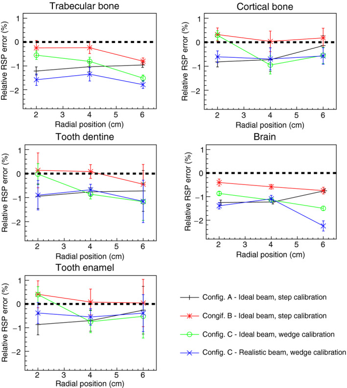
Comparison of RSP values reconstructed for the IP3 phantom in different configurations. The RSP relative error is calculated as the difference between reconstructed and reference values, divided by the reference value. The error bars represent the percentage relative standard deviations.

Table 3.

Mean, minimum, and maximum of the absolute value of the relative error in reconstructed RSP for the material inserts in the IP1 IP2 and IP3 phantoms in configurations A and B, using a mono‐energetic 200 MeV proton beam. The error in RSP in the IP2 phantom was significantly higher for the smallest radius in the simulation and was not considered in the calculation of the mean

Phantom	Configuration A			Configuration B
	Mean (%)	Minimum (%)	Maximum (%)	Mean (%)	Minimum (%)	Maximum (%)
IP1	0.20	0.07	0.57	0.46	0.20	0.72
IP2	0.18	0.05	0.29	0.58	0.13	1.00
IP3	0.79	0.14	1.25	0.32	0.03	0.80

4.D. Configuration B: ideal beam with single stage energy detector

The WEPL calibration curve obtained using the step phantom in configuration B is shown in Fig. 14 along with the WEPL uncertainties plotted for each one of the 41 WEPL step‐lengths. The ideal beam was used. The average WEPL error was 2.21 mm. The simple water phantom cylinder and the water phantoms IP1, IP2, and IP3 were simulated in a pCT scan. The average RSP value for the reconstructed water was 1.006 ± 0.3%. The lateral profile of the reconstructed water image is shown in Fig. 10. The maximum discrepancy from the average value was 0.93%. The results for the IP1, IP2, and IP3 phantoms are shown in Figs. 11, 12, 13. The errors for the inserts and IP1, IP2, and IP3 phantoms are summarized in Table 3.

Figure 14.

(a) The WEPL calibration curve obtained in configuration B, using the polystyrene step phantom and a mono‐energetic rectangular proton source. (b) Average single‐proton WEPL uncertainty for this configuration.

4.E. Configuration C: 5‐stage MSS, step‐phantom calibration

RSP images of the water phantom with an acrylic shell, reconstructed from measurements made with the phase II pCT scanner at NMCPC, were compared with simulations to show the degree to which the simulations accounted for experimental artifacts. The simulation was done for the NMCPC beam. A tangential slice through the center of the measured and simulated images is shown in Fig. 15. Using the WEPL calibration procedure with the step phantom led to circular artifacts in the reconstructed image and error in the reconstructed RSP up to 7% in the water region. The artifact was present in the pCT images of the phantoms with inserts as well (these simulations were done using the ideal beam). For example, the results for IP1 in configuration C and the ideal beam with the step‐phantom calibration shown in Fig. 11 show a large RSP error for the tooth dentine positioned at the center of the phantom. The new calibration procedure using the wedge phantom was developed to reduce the artifact, as shown next.

Figure 15.

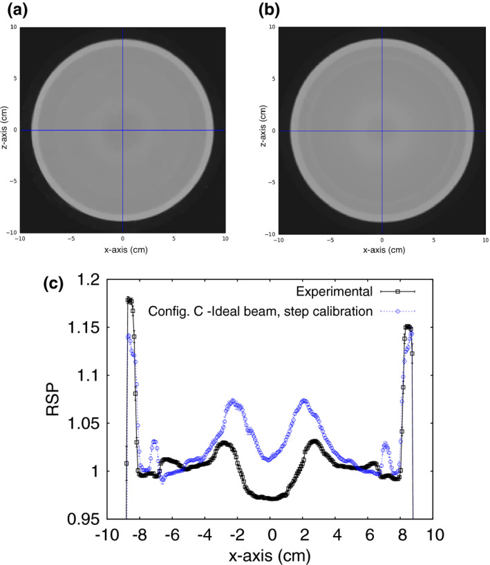
Reconstructed RSP of a water phantom for configuration C irradiated with the NMCPC beam. The images are a transverse slice through the center of the RSP image for an (a) experimental and (b) simulated scan of a water cylinder, clad in acrylic. (c) The lateral profile of the RSP averaged over the five central slices. The error bars are the standard deviation of the RSP over the five central slices. The reconstructed images have a slice thickness of 1.25 mm with 256 × 256 pixels in an evenly spaced grid with 0.78 mm spacing. The expected RSP is unity for the water region from −80 mm to 80 mm, 1.16 for the outer rim of acrylic.

4.F. Configuration C: ideal beam with 5‐stage MSS, wedge phantom calibration

The WEPL calibration curve obtained using the wedge phantom for configuration C with the ideal beam is shown in Fig. 16. The average RSP value for the reconstructed water was 1.004 ± 0.2%. The lateral profile of the reconstructed water image is shown in Fig. 10. The maximum discrepancy from the average value was 0.85%. The results for the IP1, IP2, and IP3 phantoms are shown in Figs. 11, 12, 13. The errors for the inserts and IP1, IP2, and IP3 phantoms are summarized in Table 4.

Figure 16.

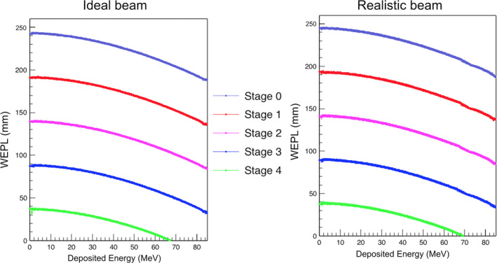
The five individual WEPL calibration curves obtained in configuration C with the polystyrene wedge phantom with ideal monoenergetic 200 MeV proton beam (left) and the realistic NMCPC beam (right).

Table 4.

Mean, minimum, and maximum of the absolute value of the relative error in reconstructed RSP for the material inserts in the IP1 IP2 and IP3 phantoms in configuration C. Results were obtained using the new wedge phantom calibration method and simulations of both the ideal beam and the realistic beam. The error in RSP in the IP2 phantom was significantly higher for the smallest radius in the simulation and was not considered in the calculation of the mean

Phantom	Configuration C with ideal beam			Configuration C with realistic beam
	Mean (%)	Minimum (%)	Maximum (%)	Mean (%)	Minimum (%)	Maximum (%)
IP1	0.22	0.01	0.36	0.34	0.05	0.63
IP2	0.47	0.10	0.81	0.41	0.10	0.78
IP3	0.79	0.02	1.52	1.02	0.38	2.24

4.G. Configuration C: realistic beam with 5‐stage MSS, wedge phantom calibration

The WEPL calibration curve obtained using the wedge phantom for configuration C with the NMCPC proton beam is shown in Fig. 16. The average RSP value for the reconstructed water was 1.004 ± 0.4%. The lateral profile of the reconstructed water image is shown in Fig. 10. The maximum discrepancy from the average value was 0.88%. The results for the IP1, IP2, and IP3 phantoms are shown in Figs. 11, 12, 13. The errors for the inserts and IP1, IP2, and IP3 phantoms are summarized in Table 4.

A transverse slice through the reconstructed image of the pediatric head phantom is shown in Fig. 17(a). In [Fig. 17(b)] RSP‐volume distributions for the reconstructed and the reference images are reported. The main peaks correspond to the RSP values of soft tissue, brain tissue, and cranium. The mean RSP values from a Gaussian fit to each of the peaks is shown in Table 5. The error in the mean reconstructed RSP, compared to the reference RSP, is under 0.2% for soft tissue and brain and 1.3% for cranium.

Figure 17.

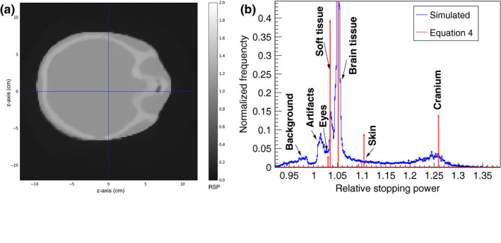
(a) A transverse slice of the reconstructed head phantom. The slice is 2 mm thick and 120 × 120 pixels, size 2 mm, were used for the reconstruction. (b) RSP‐volume distributions of the reference Eq. (4) and reconstructed RSP values for the head phantom. The normalization is such that the frequency is unity for brain tissue.

Table 5.

Mean RSP values calculated in TOPAS (reference) and reconstructed with the simulated pCT setup in configuration C, for the head phantom, using a realistic proton beam. The error is calculated as the difference between reconstructed and reference values, divided by the reference value

Material	Reference RSP	Reconstructed RSP	Standard deviation (%)	Error (%)
Soft tissue	1.035	1.037	0.4	0.17
Brain	1.051	1.051	0.19	−0.010
Cranium	1.26	1.243	2.3	−1.30

The error in range to a point located at the center of the slice shown in Fig. 17(a) was estimated for several points located around the outside of the head as shown in Fig. 18(a). Each point was located at angular steps of 20°. The water‐equivalent range for protons originating at the points around the image and stopping at the image center were estimated by adding the RSP values along the ray that connects that point with the image center. The calculation was performed for the reference RSP image and reconstructed RSP image [Fig. 18(b)]. The range calculated from the reconstructed RSP image was within 1 mm of the actual range, except at 0° at 20° where it was −1.5 mm out and at 40°, the angle showing the maximum difference of 5.3 mm.

Figure 18.

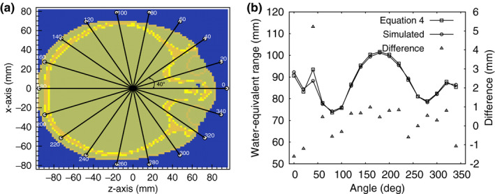
(a) A transverse slice of the reconstructed head phantom. The rays connect the center of the image with the circles around it. (b) Water‐equivalent range (left axis) as a function of the angular location of the circles shown in (a). The differences are shown in the right axis.

5. Discussion

5.A. Simulation commissioning and validation

Monte Carlo simulation provides an accurate quantitative determination of the errors associated with pCT.²⁹ In this study, the state‐of‐the‐art TOPAS tool for proton beam simulation was used to evaluate the effect of beam purity and technological complexity on pCT accuracy.

Measurements were used to accurately commission the clinically realistic uniform scanning beam at NMCPC in TOPAS. Measured and simulated beam profiles were compared for square fields of 5 cm, 10, cm and 20 cm width and were in excellent agreement, the measured field widths just under 1 mm more narrow than the simulation results (Fig. 5). For the 200 MeV, used in the pCT simulations, 20 × 10 cm² beam used for the pCT simulation, the depth penetration agreed with measurement to 0.50 ± 1.3 mm, the Bragg peak width to 0.02 ± 0.04 mm, and the peak to plateau ratio to 0.02 ± 0.06, showing the uncertainty in the Bortfeld fit. The small differences in RSP observed between results simulated with the ideal beam and clinically realistic beam (0.4% in Fig. 10) demonstrate RSP error to be insensitive to further adjustment in the details of the simulated clinical beam.

The simulation of the pCT scanner was validated with measurements made with the latest version of a prototype pCT scanner on the NMCPC uniform scanning beam with the step‐phantom calibration (Fig. 15). The central artifact in the measured image was also present in the simulated image with similar size and close to the same magnitude, with a peak to trough RSP variation of 5.7% in the measurement and 5.0% in the simulation. The wedge calibration reduced the artifact to 0.4% in the simulation (Fig. 10).

The images reconstructed from measurement and simulation when using the step‐phantom calibration agreed within 1% in RSP variation in the region of the artifact and better than 1% in RSP outside of this region out to 6.5 cm. The inserts in the different phantoms were all contained within this region. Thus, the simulated RSP error is expected to agree with measurement for the same configuration within 0.5% for the different calibration approaches and the different beams and detectors studied (Figs. 11, 12, 13, Tables 3, 4). Experimental effects not included in the simulation such as event pile‐up uncertainty (double events were detected and removed in the measurement) and conversion of absorbed dose to detector signal (optical photon transport and PMT noise, for example) are expected to have no greater than a 0.5% effect on the RSP error.

5.B. Reconstructed RSP accuracy

The uncertainties associated with the pCT reconstruction technique were determined for an ideal 200 MeV mono‐energetic beam and the 200 MeV clinically realistic beam for three configurations of the energy detector with an increasing degree of complexity (Table 2). Customized WEPL calibration curves were calculated for each configuration (Figs. 8, 14 and 16). For configuration A with ideal beam and ideal energy detector, the average single‐proton WEPL error along the penetration depth (~250 mm) was ~2 mm (Fig. 8). This resulted in an average error on the reconstructed RSP values of 0.2%, with a maximum discrepancy of 0.3% for the reconstructed image of the water phantom (Fig. 10). Similar accuracy was obtained for the IP1 phantom, as shown in Fig. 11 and Table 3. The insert material composition did not affect the accuracy on the reconstructed RSP. For the smallest inserts in the IP2 phantom (0.5 cm radius), the dimension is twice the spatial resolution of the pCT reconstruction of about 5 l p/cm,⁴⁰ the reconstructed RSP is less accurate, with error in the RSP reconstruction of ~3% for brain tissues and 9% for cortical bone (Fig. 12). The magnitude of the error is comparable in all configurations investigated. However, such errors in RSP result in a range error in water for a beam traversing 5 mm of the material (the diameter of the insert) of 0.3 mm for brain tissue and 1.6 mm bone. For the larger radius inserts, the average error was 0.2%, as for the IP1 phantom inserts (Table 3). Results for the brain and cortical bone inserts averaged at 40 mm and 60 mm from the center of the IP3 phantom were added to the plot in Fig. 12 to show the error at this intermediate insert radius of 5 mm. The error for smaller objects reduces sharply with increasing object size and becomes unimportant for long cylinders of 5 mm radius and above. There was no significant trend for the error dependence on radial position (Fig. 13).

For configuration B, with a single stage scintillator, the WEPL accuracy was 2.21 mm on average, slightly higher than the 2.08 mm obtained in configuration A. The accuracy was worse for deeper proton penetrations (comparing Figs. 8 and 14). For this configuration, the reconstructed RSP images were slightly less accurate for the water phantom, IP1 phantom and soft tissue in the IP2 phantoms, as seen in Figs. 11, 12 and Table 3. The higher RSP error is not evident in cortical bone for the IP2 phantom (Fig. 12) or for the IP3 phantom with the smaller radius cylinders (Fig. 13). The independence of RSP error on material (Fig. 11) and distance from the center of the phantom (Fig. 13), and dependence on dimension (Fig. 12) was similar in configurations A and B.

When the MSS was included in the simulation (configuration C) a more complex calibration method was necessary, involving different calibration curves for each stage and a criterion to discriminate in which stage the proton had stopped. Adoption of the original WEPL calibration, procedure developed with the step phantom,²⁰ led to artifacts in the reconstructed images and an RSP error of 7% in the center of the water phantom (Fig. 15), seen as an error in the reconstructed RSP of the central insert in the IP1 phantom (Fig. 11). For this reason, a new calibration wedge phantom was developed (see Materials and Methods section). Using this method and the ideal proton beam, results (Figs. 10, 11, 12, 13) became comparable to those of the ideal configuration A. For example, the average RSP value for the reconstructed water was 0.2%, same as in configuration A, and the maximum discrepancy from the average value was 0.85%, versus 0.3% for configuration A. In some cases, results were even more accurate than results for the single stage scintillator in configuration B.

Introduction of the more realistic NMCPC proton beam in the simulation of configuration C had minimal effect on the reconstructed RSP accuracy, with accuracy comparable to the ideal configuration A, (Figs. 10, 11, 12, 13, Table 4). For example, the average error for the IP1 phantom was found to be 0.34% versus 0.20% in configuration A.

In addition to the water phantoms, the pediatric head phantom was reconstructed in Configuration C using the NMCPC beam. All structures are well recognizable in the reconstructed image (brain, bones, air cavities, etc.) and no artifacts were visible (Fig. 17). The three main tissue materials (soft tissue, brain, and cranium) were well identifiable in the reconstructed RSP‐volume distribution (Fig. 17). In particular, brain tissue, forming the bulk of tissue in the head phantom, was reconstructed with a high degree of accuracy with a mean RSP error of only 0.02%. The higher error for the cranium is due to the small size of the bones in the skull and partial volume averaging, as seen in the increase in error for the small radius inserts in phantom IP2 (Fig. 12). The range calculated from the reconstructed RSP was within 1 mm of the actual range in most cases, with the exception of the 5.3 mm error occurring at the 40° beam angle. In this case the ray passes parallel to a bone‐soft tissue interface, a situation that is not robust in treatment planning and is generally avoided in clinical practice.

In summary, the accuracy of pCT image reconstruction for the ideal case of a 200 MeV monoenergetic proton beam where the energy detector is totally absorbing was shown to be 1.3% in RSP error for inserts of 5 mm radius or more, 0.7 mm in range for the 2.5 mm radius inserts, or better. This is the highest accuracy achievable using the current pCT calibration phantom and reconstruction algorithm. The single stage scintillator generally led to higher RSP errors. The MSS coupled with the associated calibration and reconstruction method improved the accuracy of the reconstructed RSP from the single stage scintillator result. The accuracy with this MSS and the NMCPC proton beam for the cylindrical phantoms was shown to be similar to the ideal configuration and equal to 2.2% in RSP error for inserts of 5 mm radius or more, 0.7 mm in proton range for the 2.5 mm radius inserts, or better. The pCT scan of realistic human‐like phantom resulted in clear images with no artifact. All the salient structures were well visible. The mean RSP values for the various tissues were within 1.3% of the reference ones, and the range difference for different beam angles within 1 mm for most of the directions, except in exceptional situations such as parallel incidence through an interface between low and high density tissue.

6. Conclusions

The accuracy of pCT and its dependence on beam purity and technological complexity of the pCT scanner was successfully evaluated using the Monte Carlo platform TOPAS. It proved necessary to use a wedge shaped phantom for calibration of the multi‐stage scintillator. From the results obtained, the pCT imaging technique proved to be a precise and accurate imaging tool, rivaling the current x‐ray based techniques, related to the advantage of being directly sensitive to proton stopping power rather than photon attenuation coefficients. Since the in silico results are expected to accurately represent the prototype pCT, upcoming measurements with the current prototype pCT scanner are expected to show similar accuracy in the reconstructed RSP.

Conflict of interest

The authors have no relevant conflicts of interest to disclose.

References

- 1. Moyers MF, Sardesai M, Sun S, Miller DW. Ion stopping powers and CT numbers. Med Dosim. 2010;35:179–194. [DOI] [PubMed] [Google Scholar]
- 2. Yang M, Zhu XR, Park P, et al. Comprehensive analysis of proton range uncertainties related to patient stopping‐power‐ratio estimation using the stoichiometric calibration. Phys Med Biol. 2012;57:4095–4115. [DOI] [PMC free article] [PubMed] [Google Scholar]
- 3. Han J, Siebers V, Williamson JF. A linear, separable two‐parameter model for dual energy CT imaging of proton stopping power computation. Med Phys. 2016;43:600–612. [DOI] [PMC free article] [PubMed] [Google Scholar]
- 4. Yang M, Virshup G, Clayton J, Zhu XR, Mohan R, Dong L. Theoretical variance analysis of single‐ and dual‐energy computed tomography methods for calculating proton stopping power ratios of biological tissues. Phys Med Biol. 2010;55:1343–1362. [DOI] [PubMed] [Google Scholar]
- 5. Schneider U, Pemler P, Besserer J, Pedroni E, Lomax A, Kaser‐Hotz B. Patient specific optimization of the relation between CT‐hounsfield units and proton stopping power with proton radiography. Med Phys. 2005;32:195–199. [DOI] [PubMed] [Google Scholar]
- 6. Cormack M, Koehler AM. Quantitative proton tomography: preliminary experiments. Phys Med Biol. 1976;21:560. [DOI] [PubMed] [Google Scholar]
- 7. Hanson KM. Proton computed tomography: the application of protons to computed tomography. IEEE Trans Nucl Sci. 1979;26:1635–1640. [Google Scholar]
- 8. Hanson KH, Bradbury JN, Cannon IM, et al. Computed tomography using proton energy loss. Phys Med Biol. 1981;26:965–983. [DOI] [PubMed] [Google Scholar]
- 9. Hurley RF, Schulte RW, Bashkirov VA, et al. Water‐equivalent path length calibration of a prototype proton CT scanner. Med Phys. 2012;39:2438. [DOI] [PMC free article] [PubMed] [Google Scholar]
- 10. Sadrozinski HFW, Johnson RP, MacAfee S, et al. Development of a head scanner for proton CT. Nucl Instrum Methods A. 2013;699:205–210. [DOI] [PMC free article] [PubMed] [Google Scholar]
- 11. Schulte RW, Bashkirov VA, Klock MC, et al. Density resolution of proton computed tomography. Med Phys. 2005;32:1035–1046. [DOI] [PubMed] [Google Scholar]
- 12. Sadrozinski HF‐W, Bashkirov VA, Bruzzi M, et al. Issues in proton computed tomography. Nucl Instrum Methods A. 2003;511:275–281. [DOI] [PMC free article] [PubMed] [Google Scholar]
- 13. Schulte R, Bashkirov V, Li TF, Liang ZR, Mueller K, Heimann J. Conceptual design of a proton computed tomography system for applications in proton radiation therapy. IEEE Trans Nucl Sci. 2004;51:866–972. [Google Scholar]
- 14. Li TF, Liang ZR, Singanallur JV, Satogata TJ, Williams DC, Schulte RW. Reconstruction for proton computed tomography by tracing proton trajectories: a Monte Carlo study. Med Phys. 2006;33:699–706. [DOI] [PMC free article] [PubMed] [Google Scholar]
- 15. Schulte RW, Penfold SN, Tafas JT, Schubert KE. A maximum likelihood proton path formalism for application in proton computed tomography. Med Phys. 2008;35:4849–4856. [DOI] [PubMed] [Google Scholar]
- 16. Penfold SN, Rosenfeld AB, Schulte RW, Schubert KE. A more accurate reconstruction system matrix for quantitative proton computed tomography. Med Phys. 2009;36:4511–4518. [DOI] [PubMed] [Google Scholar]
- 17. Missaghian J, Hurley F, Bashkirov V, et al. Beam test results of a CsI calorimeter matrix element. J Instrum 5. 2010;P06001:1–12. [Google Scholar]
- 18. Coutrakon G, Bashkirov V, Hurley F, et al. Design and construction of the first proton CT scanner. Appl Accelerators Res Ind. 2013;1525:327–331. [Google Scholar]
- 19. Penfold SN, Rosenfeld AB, Schulte RW, Sadrozinksi HF‐W. Geometrical optimization of a particle tracking system for proton computed tomography. Radiat Meas. 2011;46:2069–2072. [Google Scholar]
- 20. Johnson RP, Bashkirov V, DeWitt L, et al. A fast experimental scanner for proton CT: technical performance and first experience with phantom scans. IEEE Trans Nucl Sci. 2015;63:52–60. [DOI] [PMC free article] [PubMed] [Google Scholar]
- 21. Sadrozinski HF‐W, Geoghegan T, Harvey E, et al. Operation of the preclinical head scanner for proton CT. Nucl Instrum Methods A. 2016;831:394–399. [DOI] [PMC free article] [PubMed] [Google Scholar]
- 22. Bashkirov VA, Johnson RP, Sadrozinski HF‐W, Schulte RW. Development of proton computed tomography detectors for applications in hadron therapy. Nucl Instrum Methods A. 2016;809:120–129. [DOI] [PMC free article] [PubMed] [Google Scholar]
- 23. Bashkirov VA, Schulte RW, Hurley RF, et al. Novel scintillation detector design and performance for proton radiography and computed tomography. Med Phy. 2016;43:664–674. [DOI] [PMC free article] [PubMed] [Google Scholar]
- 24. Penfold S. Image reconstruction and Monte Carlo simulations in the development of proton computed tomography for applications in proton radiation therapy. PhD Thesis, University of Wollongong, Wollongong, Australia, 2010. [Google Scholar]
- 25. Penfold SN, Schulte RW, Censor Y, Rosenfeld AB. Total variation superiorization schemes in proton computed tomography image reconstruction. Med Phys. 2010;37:5887–5895. [DOI] [PMC free article] [PubMed] [Google Scholar]
- 26. Perl J, Shin J, Schümann J, Faddegon B, Paganetti H. TOPAS: an innovative proton Monte Carlo platform for research and clinical applications. Med Phys. 2012;39:6818–6837. [DOI] [PMC free article] [PubMed] [Google Scholar]
- 27. Agostinelli S, Allison J, Amako K, et al. GEANT4 ‐ a simulation toolkit. Nucl Instrum Methods A. 2003;506:250–303. [Google Scholar]
- 28. Allison J, Amako K, Apostolakis J, et al. Geant4 developments and applications. IEEE Trans Nucl Sci. 2006;53:270–278. [Google Scholar]
- 29. Giacometti V, Bashkirov VA, Piersimoni P, et al. Software platform for simulation of a prototype proton CT scanner, submitted to and under revision by Medical Physics. [DOI] [PMC free article] [PubMed]
- 30. Testa M, Schümann J, Lu HM, et al. Experimental validation of the TOPAS Monte Carlo system for passively scattering proton therapy. Med Phys. 2013;40:121719. [DOI] [PMC free article] [PubMed] [Google Scholar]
- 31. Schneider U, Pedroni E. Proton radiography as a tool for quality control in proton therapy. Med Phys. 1995;22:353–363. [DOI] [PubMed] [Google Scholar]
- 32. Pemler P, Besserer J, de Boer J, et al. A detector system for proton radiography on the gantry of the Paul‐Scherrer‐Institute. Nucl Instrum Methods Phys Res A. 1999;432:483–495. [Google Scholar]
- 33. Han B, Xu XG, Chen GTY. Proton radiography and fluoroscopy of lung tumors: a Monte Carlo study using patient‐specific 4DCT phantoms. Med Phys. 2011;38:1903–1911. [DOI] [PMC free article] [PubMed] [Google Scholar]
- 34. Wang D, Rockwell Mackie T Tome WA. On the use of a proton path probability map for proton computed tomography reconstruction. Med Phys. 2010;37:4138–4145. [DOI] [PMC free article] [PubMed] [Google Scholar]
- 35. Williams C. The most likely path of an energetic charged particle through a uniform medium. Phys Med Biol. 2004;49:2899–2911. [DOI] [PubMed] [Google Scholar]
- 36. Newhauser W, Zhang R. The physics of the proton therapy. Phys Med Biol. 2015;60:155–209. [DOI] [PMC free article] [PubMed] [Google Scholar]
- 37. Lee C, Lodwick D, Hurtado J, Pafundi D, Williams JL, Bolch WE. The UF family of reference hybrid phantoms for computational radiation dosimetry. Phys Med Biol. 2010;55:339–363. [DOI] [PMC free article] [PubMed] [Google Scholar]
- 38. ICRP Publication 110 Adult reference computational phantoms. 30(2), 2009. [DOI] [PubMed]
- 39. Bortfeld T. An analytical approximation of the Bragg curve for the therapeutic proton beams. Med Phys. 1997;24:2024–2033. [DOI] [PubMed] [Google Scholar]
- 40. Plautz T, Johnson R, Sadrozinski H, et al. An evaluation of spatial resolution of a prototype proton CT scanner, accepted for publication by Medical Physics. [DOI] [PMC free article] [PubMed]
- 41. ICRP 23 , Report of the task group on reference man, 1975. [DOI] [PubMed]
- 42. Woodart HQ, White DR. The composition of body tissues. Br J Radiol. 1986;59:1209–1219. [DOI] [PubMed] [Google Scholar]
- 43. ICRU Report 46 Photon, electron, proton and neutron interaction data for body tissue, 1991.