Compact Graph based Semi-Supervised Learning for Medical Diagnosis in Alzheimer's Disease

Abstract

Dementia is one of the most common neurological disorders among the elderly. Identifying those who are of high risk suffering dementia is important for early diagnosis in order to slow down the disease progression and help preserve some cognitive functions of the brain. To achieve accurate classification, significant amount of subject feature information are involved. Hence identification of demented subjects can be transformed into a pattern classification problem. In this letter, we introduce a graph based semi-supervised learning algorithm for Medical Diagnosis by using partly labeled samples and large amount of unlabeled samples. The new method is derived by a compact graph that can well grasp the manifold structure of medical data. Simulation results show that the proposed method can achieve better sensitivities and specificities compared with other state-of-art graph based semi-supervised learning methods.

I. Introduction

Dementia is one of the most common neurological disorders among the elderly, which can cause a progressive decline in cognitive functions. With the growth of the older population, its prevalence is expected to increase [1]. For example, Alzheimer's disease is a fatal, neurodegenerative disorder that currently affects over five million people in the U.S. It leads to substantial, progressive neuron damage that is irreversible, which eventually causes death. The current annual cost of AD care in the U.S. is more than $100 billion, which will continue to grow fast. Hence early diagnosis of AD is of great clinical importance, because disease-modifying therapies given to patients at the early stage of their disease development will have a much better effect in slowing down the disease progression and helping preserve some cognitive functions of the brain. To separate probably or possibly demented patients from normal persons, some medical data with features for describing symptoms are required [1]. Hence identifying the demented subjects can be transformed into a pattern classification problem.

To handle the pattern classification problem, the conventional supervised learning algorithms, such as LDA and its variants [11] [12], require sufficient number of labeled samples in order to achieve satisfying sensitivities and specificities. However, labeling large number of samples is time-consuming and costly. On the other hand, unlabeled samples are abundant and can be easily obtained in the real world. Hence semi-supervised learning algorithms (SSL), which incorporate partly labeled samples and a large amount of unlabeled samples into learning, have become more effective than only relying on supervised learning. Recently, based on the clustering and manifold assumptions, i.e. nearby samples (or samples on the same data manifold) are likely to share the same label, graph based semi-supervised learning algorithms have been widely used in many applications. Typical algorithms include Gaussian Fields and Harmonic Functions (GFHF) [2], Learning with Local and Global Consistency (LLGC) [3] and General Graph based Semi-supervised Learning (GGSSL) [4] [5].

The GFHF has elegant probabilistic explanation and the output labels are the probabilistic values, but it cannot detect the outliers in data; in the contrast, LLGC can detect outliers, but its output labels are not probabilistic values. Both the problems in GFHF and LLGC have been eliminated by GGSSL, in which it can either detect the outliers or develop a mechanism to calculate the probabilities of data samples. In this letter, motivated by the framework of GGSSL, we develop an effective semi-supervised learning method, namely Compact Graph based SSL, based on a newly proposed compact graph. We then model the proposed CGSSL for medical diagnosis.

The main contribution of this paper is as follows: 1) we propose a compact graph for semi-supervised learning. The newly proposed graph can represent the data manifold structure in a more compact way; 2) we model the CGSSL method for Medical Diagnosis, which can classify the patients as suffering from dementia or not. Simulation results show that the proposed CGSSL can achieve better classification performance compared with other graph based semi-supervised learning methods.

II. The Proposed Semi-Supervised Methods

A. Review of Graph Construction

In label propagation, a similarity matrix must be defined for evaluating the similarities between any two samples. The similarity matrix can be approximated by a neighborhood graph associated with weights on the edges. Officially, let G̃ = (Ṽ, Ẽ) denote this graph, where Ṽ is the vertex set G̃ of representing the training samples, Ẽ is the edge set of G̃ associated with a weight matrix W containing the local information between two nearby samples. There are many ways to define the weight matrix. A typical way is to use Gaussian function [1]–[5]:

$$w_{ij}=\exp \left(-{\Vert x_i-x_j\Vert }^2∕2{\sigma }^2\right)x_i\in N_k\left(x_j\right)or{x}_j\in N_k\left(x_i\right),$$ (1)

where N_k (x_j)is the k neighborhood set of x_j, σ is the Gaussian function variance. However, σ is hard to be determined and even a small variation of σ can make the results dramatically different [7]. Wang et al. have proposed another strategy to construct G by using the neighborhood information of samples [7][8]. This strategy assumes that each sample can be reconstructed by a linear combination of its neighborhoods [9], i.e. $x_i\approx {\sum }_{j:x_j\in N_k\left(x_i\right)}{w}_{ij}{x}_j$. It then calculates the weight matrix by solving a standard quadratic programming (QP) problem as:

$$\min {\Vert x_i-\sum _{j:x_j\in N_k\left(x_i\right)}{w}_{ij}{x}_j\Vert }_F^{2}s.t.w_{ij}\ge 0,\sum _{j\in N_k\left(x_i\right)}{w}_{ij}=1.$$ (2)

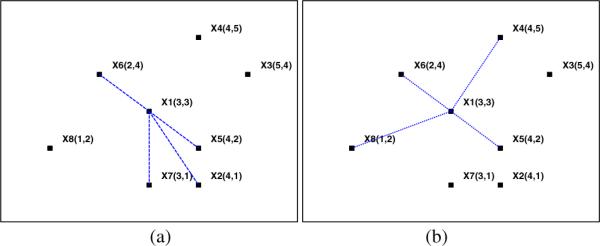
The above strategy is empirically better than the Gaussian function, as the weight matrix can be automatically calculated in a closed form once the neighborhood size is fixed. However, using the neighborhoods of a sample to reconstruct it may not achieve a compact result [6]. We use Fig. 1 to elaborate this fact, in which we generalize eight samples in R². We then, in this next subsection, propose a more effective strategy for graph construction.

Fig. 1.

Two ways for reconstruct x1: seven data points with coordinates as: x₁ (3,3), x₂ (4,1), x₃ (5,4), x₄ (4,5), x₅ (4,2), x₆ (2,4), x₇ (3,1) and x₈ (1,2) (a) reconstruct using the neighbors of x₁ (b) reconstruct x₁ using the neighbors of x₆.

Taking x₁as an example and let k = 5, we first reconstruct x₁ by using its neighborhoods, i.e. {x₁, x₅, x₆, x₇, x₂}. Following Eq. (2), we have $\widetilde{x_1}=0.1694x_5+0.2491x_6+0.4109x_7+0.1706x_2$. In this case, the reconstruction error is ${\Vert x_1-\widetilde{x_1}\Vert }_F^2=0.26852$. Note that x₁ is also in the neighborhoods of x₆, i.e. {x₆, x₁, x₄, x₈, x₅}. Hence if we use them, i.e. {x₆, x₄, x₈, x₅}, to reconstruct x₁ as $\widetilde{x_1}=0.1669x_6+0.2223x_4+0.2223x_8+0.3884x_5$, the error can be 0.04631 < 0.26853. This indicates that using the neighborhoods of x₆ to reconstruct x₁ is better than that using the neighborhoods of its own, as the former reconstruction error is much smaller.

B. The Proposed Graph Construction

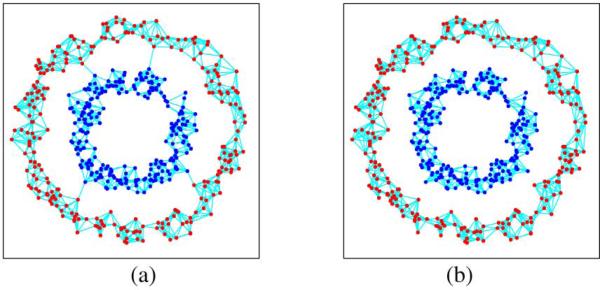
The above analysis motivates us to propose an improved local reconstruction strategy for graph construction. Since the minimum reconstruction error of a sample may not be obtained by its own neighborhood, we need to search in its adjacent samples and find the minimum error. This can be a more compact way to reconstruct each sample. In practice, we first generate a vector ε = [ε₁, ε₂, . . . , ε_l+u] ∈ R^{1 ×(l+u)}to preserve the minimum errors of samples. We then search each sample x_j and its neighborhood set N_j : x_j1, x_j2, . . . , x_jk(including itself). For each x_ji, i = 1 to k, we use other samples in N_j to reconstruct it. If the reconstruction error $\widetilde{{\epsilon }_{j_i}}$ is smaller than ε_ji preserved in ε, replace ε_ji with $\widetilde{{\epsilon }_{j_i}}$ and preserve the reconstruction weights x_ji of into W. The basic steps of the proposed strategy can be shown in Table I. We also give an example in Fig. 2 to show the improvement of the proposed graph construction, in which we display the merit of our graph construction approach on a two-cycle dataset.

TABLE I.

An Improved Method to Calculate Reconstructed Weight

Input:

Data matrix X ∈ RD×(l+u), neighborhood number k.

Output:

Weight matrix W = [x1, x2,..., xl+u] ∈ R(l+u)×(l+u).

Algorithm:

1. Generate an error vector ε = [ε1, ε2,..., εl+u] ∈ R1×(l+u) with each element εj = +∞ and initialize W as a zero matrix.

2. for each sample xj, j = 1 to l + u, do

3. Identify the k neighborhood set as: Nj : xj1, xj2, ..., xjk.

4. for each sample xji, i = 1 to k, do

5. Reconstruct $x_{j_i}\approx x_{j_i}={\sum }_{t:t=1:k,t\ne i}{w}_{j_t}{x}_{j_t}$ following Eq. (2).

6. if the reconstructed error ${\epsilon }_{j_i}={\Vert x_{j_i}-x_{j_i}\Vert }_F^2<{\epsilon }_{j_i}$, do

7. ${\epsilon }_{j_i}\leftarrow \widetilde{{\epsilon }_{j_i}}$, clear the ji th column of W and update it by wjt, t = 1 to k, t ≠ i, which are obtained in Step 5.

8. end for

9. end for

10. output weight matrix W

Fig. 2.

Two ways to construct the graph: two-cycle dataset (a) using the strategy of Wang et al. [7], the total reconstructed error is 12.29283; (b) using the strategy of the proposed method, the total reconstructed error is 0.00039. From the results, we can see the proposed strategy can construct the graph in a compact way.

C. Symmetrization and Normalization of Graph Weight

Note that the improved local reconstruction weight W obtained by Table I does not satisfy the symmetric property, i.e. W ≠ W^T, which means it does not have a close relationship to the graph theorem. Though this drawback can be overcome by the symmetry process, i.e. W ←(W + W^T), the weight matrix still holds inhomogeneous degrees. In our work, to handle this problem, we design the proposed weight matrix as follows:

$$\tilde{W}=W{\Delta }^{-1}{W}^T.$$ (3)

where Δ ∈ R^{(l+u) × (l+u)} is a diagonal matrix with each element Δ_jj being the sum of the jth row in W, i.e. ${\Delta }_{jj}={\sum }_{i=1}^{l+u}{W}_{ij}$. It can be easily verified that W̃ is symmetric. In addition, the sum of each row or column of W̃ is equal to 1, hence W̃ is also normalized. As pointed in [4], the normalization can strengthen the weights in the low-density region and weaken the weights in the high density region, which is advantageous for handling the case in which the density of datasets varies dramatically. Following Eq. (3), it can be noted that by neglecting the diagonal matrix Δ, WW^T is an inner product with each element (WW^T)_ij measuring the similarity between each pair-wise local reconstructed vector w_i and w_j. Given x_i and x_j are close to each other and in the same manifold, their corresponding w_i and w_i tends to be similar and (WW^T)_ij will be a large value; otherwise, (WW^T)_ij will be equal to 0, if x_i and x_j are not in the same neighborhood. The weight matrix defined in Eq. (3) can also be easily extended to out-of-sample data by using the same smoothness criterion. We will discuss this issue in Section II-E.

D. Label Propagation Process

We will then predict the labels of unlabeled samples based on a general graph based semi-supervised learning process (GGSSL) [4] [5]. Let Y = [y₁, y₂, . . . , y_l+u] ∈ R^{(c+1) × (l+u)} be the initial labels of all samples, for the labeled sample x_j, y_ij = 1 if x_j belongs to the ith class, otherwise y_ij = 0; for the unlabeled sample x_j, y_ij if i = c + 1, otherwise y_ij = 0. Note that an addition class c + 1 is added to represent the undetermined labels of unlabeled samples hence the sum of each column of Y is equal to 1 [4]. We also let F = [f₁, f₂, . . . , f_l+u] ∈ R^{(c+1) × (l+u)} be the predicted soft label matrix, where f_i are row vectors satisfying 0 ≤ f_ij ≤ 1.

Consider an iterative process for label propagation. At each iteration, we hope the label of each labeled sample is partly received from its neighborhoods and the rest is from its own label. Hence the label information of the data at t + 1iteration can be:

$$F(t+1)=F\left(t\right)\tilde{W}{I}_{\alpha }+Y{I}_{\beta }.$$ (4)

where I _α ∈ R^{(l+u) × (l+u)} is a diagonal matrix with each element being α_j, I_β = I – I_α, α_j (0 ≤ α_j ≤ 1) is a parameter for x_j to balance the initial label information of x_j and the label information received from its neighbors during the iteration. According to [4], the regularization parameter α_j for the labeled data x_j is set to α_l; for the unlabeled sample x_j, it is set to α_u in the simulations. In this paper, we simply set α_l = 0 for labeled sample, which means we constrain F^l = Y_l, and set the value of α_u for unlabeled sample. The iterative process of Eq. (4) converges to:

$$F={\lim }_{t\to \infty }F\left(t\right)=Y{I}_{\beta }{\left(I-\tilde{W}{I}_{\alpha }\right)}^{-1}.$$ (5)

It can be easily proved that the sum of each column F of is equal to 1 [4][5]. This indicates that the elements in F are the probability values and f_ij can be seen as the posterior probability of x_j belonging to the ith class; when i = c + 1, f_ij represents the probability of x_j belonging to the outliers.

E. Out-of-sample Inductive Extension

In general, the proposed CGSSL is a transductive method, which cannot deal with out-of-sample data, i.e. it cannot predict the faulty or normal condition for a new patient. In this subsection, we will apply the local approximation strategy in Eq. (2) (3) to extend CGSSL to the out-of-sample data. Specifically, following the work in [10], we first give the smoothness criterion for the new-coming sample considering the intuition of training in Eq. (2) (3):

$$J\left(f\left(z\right)\right)=\sum _{j:x_j\in X,x_j\in N_k\left(z\right)}\tilde{w}(z,x_j){\Vert f\left(z\right)-f_j\Vert }_F^2.$$ (6)

where N_k(z) is the neighborhood set of z, w̃(z, x_j) is the similarity between z and x_j, f(z) is the predicted label of z. Note that the nearest neighbors of z, i.e. N_k(z), are retrieved from z U X, and the weight matrix w̃(z, x_j) satisfies the sum-to-one constraint, i.e. ${\sum }_{j:x_j\in X,x_j\in N_k\left(z\right)}\tilde{w}(z,x_j)=1$. Since J(f(z)) is convex in f(z), it is minimized by setting the derivation of J(f(z)) in Eq. (6) w.r.t. f(z) to zero. Then, the optimal f*(z) can be given as follows:

$$f^{\ast }\left(z\right)=\sum _{j:x_j\in X,x_j\in N_k\left(z\right)}\tilde{w}(z,x_j)f_j.$$ (7)

Here, we define the weight matrix following the same form as Eq. (2) (3). Specifically, we first calculate w(z,x_j)by the same strategy following Eq. (2), which is to minimizing the following objective function:

$$J\left(f\left(z\right)\right)={\Vert f\left(z\right)-\sum _{j:x_j\in N_k\left(z\right)}w(z,x_j)f_j\Vert }_F^{2}s.t.w(z,x_j)\ge 0,\sum _{j\in N_k\left(z\right)}w(z,x_j)=1.$$ (8)

We then extend w(z) following the same form of Eq. (3), i.e.

$$\tilde{w}\left(z\right)=\tilde{w}\left(z\right){\Delta }^{-1}{W}^T,$$ (9)

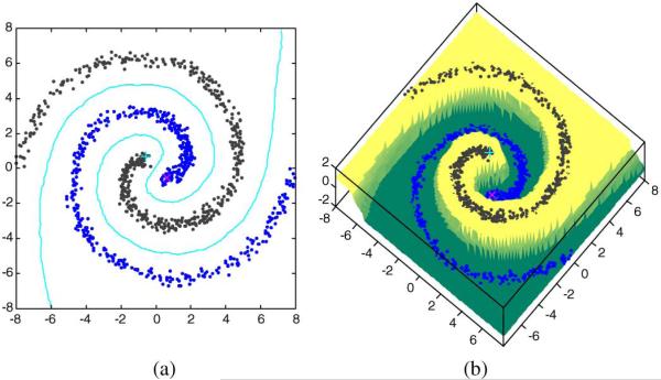
and it can be easily verified ${\sum }_{j:x_j\in X,x_j\in N_k\left(z\right)}\tilde{w}(z,x_j)=1$ A toy example for evaluating the effectiveness of the proposed out-of-sample extension can be seen in Fig. 3, where we generalize a two-Swiss-roll dataset with one sample labeled per class.

Fig. 3.

Illustration of out-of-sample extension: two-Swiss-roll dataset (a) out-of-sample results in {(x, y)|x ∈ [–8, 8], y ∈ [–8, 8]} using Table 3. The contour lines represent boundary between two classes form by the data points with the estimated label values equal to 0 (b) The z-axis indicates the predicted label values associated with different colors over the region.

III. Simulation

A. Data Description

The proposed method will be evaluated by the demented subjects who meet the criteria for dementia in accordance with standard criteria for dementia of the Alzheimer's type or other non-Alzheimer's demented disorders in their first visits to Alzheimer disease Centers (ADCs) throughout the United States. Data from 289 demented subjects and 9611 controls collected by approximately 34ADCs from 1994 to 2011 are studied. These data are organized and made available by the US National Alzheimer's Coordinating Center (NACC). Among the demented patients studied, 97% of them were classified as probable or possible Alzheimer's disease (AD) patients. Those with dementia and with neither probable AD nor possible AD have other types of dementia such as Dementia with Lewy Bodies, and Frontotemporal Lobar Degeneration. 5 nominal, 142 ordinal, and 9 numerical attributes of the subjects are included in the study. These attributes include demographic data, medical history, and behavioral attributes, with 5% being missing values. To make the classification problem more diffi-cult, cognitive assessment variable, such as Mini-Mental State Examination score, is not included in the current analysis.

B. Model Stage

This stage is used to identify whether a case in NACC dataset belongs to an AD patient, i.e. to estimate the probability of a case belonging to the AD patient. In practice, we may get some prior information about which cases in NACC are AD patient or not. We then label such cases to form the labeled matrix and our goal is to propagate the label information from the known cases to the unknown cases. Here, for each case x_j, we define its label vector as y_j = {a_j, n_j, p_j}^T representing the probabilities of x_j belongings to AD patient, non-AD person and possible AD patient. Specifically, if x_j belongs to AD patient, we set a_j = 1 and n_j = p_j = 0; if x_j belongs to non-AD person, we set n_j = 1 and a_j = p_j = 0; if x_j is an unlabeled case, we treat it as possible AD patient and set p_j = 1 and a_j = n_j = 0. After we define the label matrix, we can use it to estimate the labels of the unlabeled cases by the proposed CGSSL.

C. Simulation Results

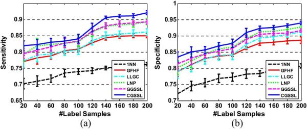
We compare the performances of CGSSL with other state-of-art graph based semi-supervised learning algorithms such as GFHF [2], LLGC [3], GGSSL [4] [5] and LNP [7]. We also compare with one nearest neighbor classifier (1NN) as a baseline. In this simulation, we randomly choose 20-200 samples per class as labeled set and the remaining as unlabeled set. We then perform different methods and the class label of unlabeled sample $x_j^u$ is determined by $x_j^u=\arg {\max }_i{f}_{ij}^u$. To evaluate the performance of different algorithms, we use sensitivity and specificity for statistically measuring the binary-class classification accuracies. Other parameters are set with the same strategy as in [4].

The average sensitivities and specificities over 20 random splits of different SSL methods are in Fig. 4. From the simulation results, we can obtain the following observations: 1) all semi-supervised learning methods outperform 1NN by about 4%–6%. For example, the proposed CGSSL can achieve 8% improved sensitivities and 6% specificities to 1NN, respectively; 2) for most semi-supervised learning methods such as GFHF and LLGC, they achieve higher specificities than sensitivities. For example, the specificities of GFHF and LLGC are higher than their sensitivities by about 1%–2%. 3) Among all semi-supervised learning methods, the proposed CGSSL can achieve the best performances due to the reason as analyzed in Section II-B.

Fig. 4.

The average sensitivities and specificities over 20 random splits of different SSL methods: (a) sensitivities; (b) specificities.

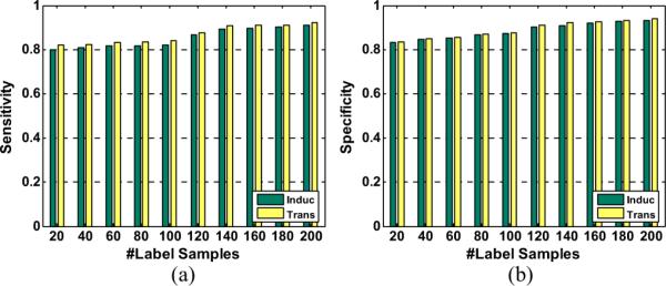
We also compare the performances between the proposed CGSSL and out-of-sample inductive method with different number of labeled samples. In this simulation, we randomly select 2000 samples from unlabeled samples to form the test set. Since CGSSL itself cannot be used to deal with testing samples, we regard testing samples as unlabeled and integrate them for training. The simulation results are given in Fig. 5. It is obvious that the inductive extension of CGSSL can achieve similar performance as the transductive version. It is natural that the transductive method performs a little better than its inductive extension since we have considered testing samples as unlabeled samples in transductive CGSSL.

Fig. 5.

The comparison between transductive and inductive methods (out-of sample extension): (a) sensitivities; (b) specificities.

IV. Conclusion

Dementia is one of the most common neurological disorders among the elderly. Identification of demented patients from normal subjects can be transformed into a pattern classification problem. In this letter, we introduce an effective semi-supervised learning algorithm, which is based on a newly proposed graph. The newly proposed graph can represent the data manifold structure in a more compact way. We then model the proposed CGSSL algorithm for Medical Diagnosis. To the best of our knowledge, this letter can be the first work that utilizes graph based semi-supervised learning into medical diagnosis. Simulation results show that the proposed CGSSL can achieve better classification performance compared with other graph based semi-supervised learning methods.

TABLE II.

The Method of CGSSL and Out-of-Sample Extension

Input: Data matrix X ∈ RD×(l+u), label matrix Y ∈ R(c+1)×(l+u), the number of nearest neighbor k and other relative parameters.

Output: The predicted label matrix F ∈ R(c+1)×(l+u).

The Transductive Method of GCSSL:

1. Construct the neighborhood graph and calculate the weight matrix W as Table 1.

2. Symmetrize and normalize W as W̃ = WΔ−1WT in Eq. (3).

3. Calculate the predicted label matrix F as Eq. (5) and output F.

Out-of-sample Inductive Extension:

1. Search the k nearest neighbor of z in $z\cup X$.

2. Construct the weight vector following Eq. (8).

3. Extend the weight vector following Eq. (9).

4. Calculate the predicted label of z as Eq. (7) and output f(z).

References

- 1.Beekly D, et al. The national alzheimer's coordinating center (NACC) database: The uniform data set. Alzheimer Dis. Assoc. Disord. 2007;21(3):249–258. doi: 10.1097/WAD.0b013e318142774e. [DOI] [PubMed] [Google Scholar]
- 2.Zhu X, Ghahramani Z, Lafferty JD. Semi-supervised learning using gaussian fields and harmonic function. Proc. ICML. 2003.
- 3.Zhou D, Bousquet O, Lai TN, Weston J, Scholkopf B. Learning with local and global consistency. Proc. NIPS. 2004.
- 4.Nie F, Xiang S, Liu Y, Zhang C. A general graph based semi-supervised learning with novel class discovery. Neural Comput. Applicat. 2010;19(4):549–555. [Google Scholar]
- 5.Nie F, Xu D, Li X, Xiang S. Semi-supervised dimensionality reduction and classification through virtual label regression. IEEE Trans. Syst., Man, Cybern. B. 2011;41(3):675–685. doi: 10.1109/TSMCB.2010.2085433. [DOI] [PubMed] [Google Scholar]
- 6.Xiang S, Nie F, Pan C, Zhang C. Regression reformulations of LLE and LTSA with locally linear transformation. IEEE Trans. Syst., Man, Cybern. B. 2011;41(5):1250–1262. doi: 10.1109/TSMCB.2011.2123886. [DOI] [PubMed] [Google Scholar]
- 7.Wang F, Zhang C. Label propagation through linear neighborhoods. IEEE Trans. Knowl. Data Eng. 2008;20(1):55–67. [Google Scholar]
- 8.Wang J, Wang F, Zhang C, Shen HC, Quan L. Linear neighborhood propagation and its applications. IEEE Trans. Patt. Anal. Mach. Intell. 2009;31(9):1600–1615. doi: 10.1109/TPAMI.2008.216. [DOI] [PubMed] [Google Scholar]
- 9.Roweis S, Saul L. Nonlinear dimension reduction by locally linear embedding. Science. 2000;290:2323–2326. doi: 10.1126/science.290.5500.2323. [DOI] [PubMed] [Google Scholar]
- 10.Delalleau O, Bengio Y, Le Roux N. Efficient non-parametric function induction in semi-supervised learning. Proc. Workshop AISTATS. 2005.
- 11.Zhao M, Chan RHM, Tang P, Chow TWS, Wong SWH. Trace ratio linear discriminant analysis for medical diagnosis: A case study of dementia. IEEE Signal Process. Lett. 2013;5(20):431–434. doi: 10.1109/LSP.2013.2250281. [DOI] [PMC free article] [PubMed] [Google Scholar]
- 12.Fukuaga K. Introduction to statistical pattern classification. Patt. Recognit. 1990 Jul.30(7):1145–1149. [Google Scholar]