Abstract
In humans, vertical posture acquisition caused several changes in bones and muscles which can be assumed as verticalization. Pelvis, femur, and vertebral column gain an extension position which decreases muscular work by paravertebral muscles in the latter. It’s widely known that six different morphological categories exist; each category differs from the others by pelvic parameters and vertebral column curvatures. Both values depend on the Pelvic Incidence, calculated as the angle between the axes passing through the rotation centre of the two femur heads and the vertical axis passing through the superior plate of the sacrum. The aim of this study is to evaluate the distribution of stress and the resulting strain along the axial skeleton using finite element analysis. The use of this computational method allows performing different analyses investigating how different bony geometries and skeletal structures can behavior under specific loading conditions. A computerized tomography (CT) of artificial bones, carried on at 1.5 mm of distance along sagittal, coronal and axial planes with the knee at 0° flexion (accuracy 0.5 mm), was used to obtain geometrical data of the model developed. Lines were imported into a commercial code (Hypermesh by Altair®) in order to interpolate main surfaces and create the solid version of the model. In particular six different models were created according Roussoly’s classification, by arranging geometrical position of the skeletal components. Loading conditions were obtained by applying muscular forces components to T1 till to L5, according to a reference model (Daniel M. 2011), and a fixed constrain was imposed on the lower part of the femurs. Materials were assumed as elastic with an Elastic modulus of 15 GPa, a Shear Modulus of 7 GPa for bony parts, and an Elastic modulus of 6 MPa, a Shear Modulus of 3 MPa for cartilaginous parts. Six different simulations have been carried out in order to evaluate the mechanical behavior of the human vertebral column arranged according to the Russoly’s classification; results confirm higher solicitations obtained varying configurations from case I to case VI. In particular way, first three cases seem to supply the different loading configurations spreading stresses in almost all the bony parts of the column, while the remaining others three cases produce an higher concentration of stress around the lower part of spine (L3, L4, L5). Results confirm a good agreement with those present in literature (Winkle et al., 1999), an equivalent Von Mises average stress was of 0,55 MPa was found on the intervertebral disks with the higher values reached on the lower part of the column. A comparison of results obtained for Case I with literature (Galbusera et al., and El Rich et al., 2004), shows a good agreement in terms of normal compressive force, while more evident differences with Galbusera’s results can be found for shear force and sagittal moment. The results underline a relationship between PI increase, and accordingly of PT and LL, and the distribution of load forces. Load forcesi is exerted mainly on distal vertebrae, especially on L4 and L5.
Keywords: Sagittal Balance, Sagittal Alignment, Finite Element Analysis, Biomehcanics, Lumbar Spine
1. Introduction
Different studies coming from various branches of science, from Paleontology to comparative anatomy suggest that vertebrates which adopt a bipedal stance apply different methods to obtain balance by an efficient distribution of weight. Several works describe this biomechanical topic in dinosaurs and birds which are also linked by a conductive line from a phylogenetic point of view Balance is reached thanks to a tail which helps these animals to have and effective distribution of the forces. The evolution led, In Apes and humans, to a progressive reduction of tail; on the other hand the vertebral column, with his shape, pledges a successful weight distribution.1
Vertebral column reflects functional demands so when a change occurs in phylogenesis is synonymous of new condition to face and to be adapted to. In Tetrapods, body support is provided by the limbs, each one is connected to the vertebral column which suspends the weight of the body. The main biomechanical issue is that the vertebral column distributes the force on the hind limbs as a bridge on the piers: Various authors compared the vertebral column with a Forth-Bridge, thus the bones resist compression forces while the muscles and ligaments are accountable to withstand the tension forces.2 Our attention is focused on bipedal dinosaurs such us the iguanodon which balances the weight of the thorax and anterior body with a heavy tail following the scheme of a seesaw, the fulcrum is located at the hip. The transition from water to land changes the function of the tail: while in fishes it is a propulsory structure in tetrapods and also in bipedal dinosaurs, an heavy tale balances the weight.The function of the tail during evolution from theropods to birds varies again.3 Vertebral column in birds is a fascinating example of duality between structure and function. The cervical region is made of numerous vertebrae flexibly articulated each other this allow a great freedom of movement to the head and neck regions;moreover vertebrae from the lumbar and sacral region are fused each other and to the pelvic girdle, thus a stable control during flight is guaranteed. Birds are the only example of stable bipedalism together with human while other species, such us Chimpanzees, adopt the erect posture only in few situations and for a restricted period of time. Chimpanzees use their arms especially to balance the weight; the assumption of a stable erect posture typical of humans has to be attributed to a verticalisation and broadening of the Pelvis.4 In humans, vertical posture acquisition caused several changes in bones and muscles which can be assumed as verticalization. Pelvis and femur and vertebral column gain an extension position which decreases muscular work by paravertebral muscles in the latter. Vialle formula explains the way the curvatures of the Vertebral column allow forces unloading. In humans, Pelvisis subjected both in its shape and position: it is retroverse in order to take to the minimum the muscular work of hip extensors during erect position. There is moreover an ileus extention due to the role of the great gluteus as an extensor and a posterior extention of Ischium tuberosity (due to hamstring function). The femur aligns itself with the previous strucutures too: verticalization of pelvis requires a more vertical oriented acetabulum. Thus bipodalism requires longer and more vertical femur than quadrupeds. Complete Knee extension surely contributed to verticalization of the femur along with femur-offset (in human the degree it’s more antiverse by 5° than in African apes). It’s widely known that six different morphological categories exist; each category differs from the others by pelvic parameters and vertebral column curvatures. Both values depend on Pelvic incidence which is the degree between the axies passing through the rotating centre of the two femur heads and the vertical axis passing through the superior plate of the sacrum. Once the development of the individual is arrested, Pelvic incidence will not be subject of variations.5, 6
The aim of this study is to evaluate the distribution of stress and the resulting strain along the axial skeleton using finite element analysis. The use of this computational method allows to perform different analyses investigating how different bony geometries and skeletal structures can behavior under specific loading conditions.
2. Material and methods
2.1. Sagittal balance morphotypes
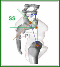
Pelvic Index can be assumed as an anatomical/morphological degree which remains stable once skeletal maturity is reached. During sagittal balance evaluation,Pelvic Index is fundamental because average values of all the other parameters depends on it. This value could assume very high values ranging from 33° to 85°,7 due to this variations, six categories had been suggested to subdivide population Table 1.8 Sacral Slope represents Sacrum declivity; on the other hand Pelvic tilt represents pelvic declivity; Pelvic Index is the sum between the two, when SS increases, PT decreases and viceversa. The relation between these parameters is shown in the Table 1. Lumbar curvatures (lumbar lordosis LL, Thoracic Kyphosis KT, Cervical lordosis), as pelvic degrees, depend on PT values as reported in Table 1.
Table 1.
Geometrical characteristics of the six FE models.
| CASE I | [28° < PI < 37,9°] | CASE IV | [58° < PI < 67,9°] | |
 |
KT = 44° LL = 55° SS = 30° PT = 4° PI = SS + PT = 34° |
 |
KT = 47° LL = 70° SS = 46° PT = 16° PI = SS + PT = 62° |
|
| CASE II | [38° < PI < 47,9°] | CASE V | [68° < PI < 77,9°] | |
 |
KT = 50° LL = 50° SS = 35° PT = 8° PI = SS + PT = 43° |
 |
 |
KT = 46° LL = 70° SS = 50° PT = 25° PI = SS + PT = 75° |
| CASE III | [48° < PI < 57,9°] | CASE VI | [78° < PI < 87,9°] | |
 |
KT = 47° LL = 65° SS = 40° PT = 12° PI = SS + PT = 52° |
 |
KT = 44° LL = 75° SS = 60° PT = 24° PI = SS + PT = 84° |
2.2. FE model
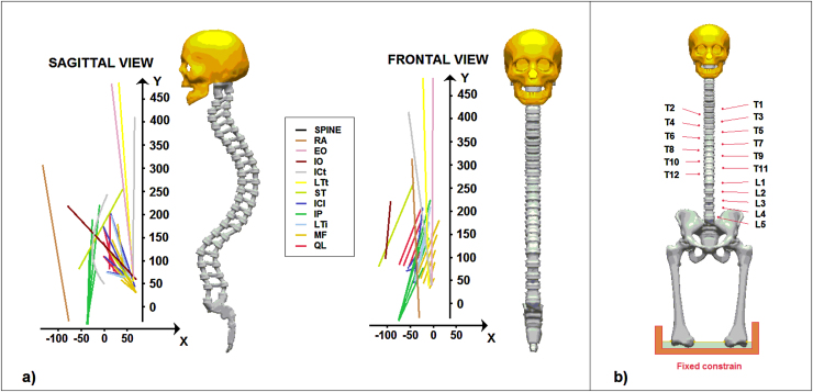
A computerized tomography (CT) of artificial bones, carried on at 1.5 mm of distance along sagittal, coronal and axial planes with the knee at 0° flexion (accuracy 0.5 mm), was used to obtain geometrical data of the model developed. Lines were imported into a commercial code (Hypermesh by Altair®) in order to interpolate main surfaces and create the solid version of the model. In particular six different models were created according Russoli's classification, by arranging geometrical position of the skeletal components, see further paragraph. Loading conditions were obtained by taking into account the point of insertion of the following muscles: Rectus Abdominis (RA), External Obliques (EO), Internal Obliques (IO), Iliocostalis thoracis pars thoracis (ICt), Longissimus thoracis pars thoracis (LTt), Spinalis thoracis (ST), iliocostalis lumborum pars lumborum (ICl), Iliopsoas (IP), Longissimus thoracis pars lumbalis (LTl), Multifidus (MF), Quadratus lumborum (QL), as described in the reference model.9 A fixed constrain was imposed on the lower part of the femurs, and the resultants of the muscular forces were applied at T1 till to T12 and at L1 till to L5, see Fig. 1. Contribution of head [39,25 N] was loaded on T1, while the weight of the arms [36,75 N] was spread among T1 till to T6. Femural connections were modeled as ilio-femural, ischiofemural and pubo-femural ligaments.
Fig. 1.
a) Sagittal and frontal views of the muscular forces aging on the model; b) FE model representation with loaded bony components and fixed constrain.
In Table 2 are reported numbers of nodes and elements employed to reproduce each part of the model, and the corresponding loading force or constrain applied.
Table 2.
Representation of loading conditions and fixed displacement applied to the different parts of the model.
| Element | Nodes | Load [N]/Fixed Constrain |
|
|---|---|---|---|
| T1 | 709 | 249 | 49,78 |
| T2 | 701 | 252 | 10,89 |
| T3 | 711 | 254 | 11,21 |
| T4 | 674 | 245 | 11,59 |
| T5 | 721 | 252 | 11,91 |
| T6 | 734 | 252 | 12,25 |
| T7 | 704 | 248 | 6,48 |
| T8 | 665 | 234 | 6,86 |
| T9 | 609 | 229 | 7,24 |
| T10 | 718 | 247 | 7,56 |
| T11 | 666 | 238 | 7,92 |
| T12 | 612 | 230 | 8,26 |
| L1 | 644 | 237 | 8,62 |
| L2 | 668 | 241 | 8,94 |
| L3 | 558 | 217 | 9,32 |
| L4 | 567 | 263 | 9,64 |
| L5 | 603 | 274 | 10,04 |
| Pelvis | 11,414 | 3589 | \ |
| Femural ligam. | 868 | 426 | \ |
| Femur | 40,192 | 10,024 | fixed constrain |
Materials were assumed as elastic with an Elastic modulus (E) of 15 GPa, a Shear Modulus (G) of 7 GPa for bony parts, and an Elastic modulus (E) of 6 MPa, a Shear Modulus (G) of 3 MPa for cartilagineus parts.
3. Results
Six different simulations have been carried out in order to evaluate the mechanical behavior of the human vertebral column arranged according to the Russoly's classification. The linear elastic analyses were performed by applying loads to the vertebral components and fixing the condilar area of the femur.10, 11 In Table 3 are reported results in terms of global displacement, equivalent elastic strain, normal force, shear force, moment, and equivalent von mises stress referred to the complete six models and to the single parts of it. As it can be argued results confirm higher solicitations obtained varying configurations from case I to case VI. In particular first three cases seem to behave in a similar manner respect to the IV, V, VI cases which show a different stress an strain shielding configuration.
Table 3.
Results in terms of global displacement, equivalent elastic strain, normal force, shear force, moment, and equivalent von mises stress referred to the complete six models.
| Displacement [mm] |
Equiv. Strain [μmm/mm] | N [N] |
S [N] |
M [N mm] |
Von Mises Stress [MPa] |
|
|---|---|---|---|---|---|---|
| CASE I | ||||||
| Complete model | 7,36E+00 | 6,98E−04 | 6,10E+02 | 3,08E+02 | −8,75E+00 | 1,98E+01 |
| T12 | 5,87E+00 | 2,77E−04 | 3,50E+02 | −3,50E+01 | −8,75E+00 | 3,02E+00 |
| L1 | 5,54E+00 | 4,67E−04 | 4,16E+02 | −5,20E+01 | −6,93E+00 | 5,57E+00 |
| L2 | 5,13E+00 | 5,70E−04 | 4,55E+02 | −7,58E+01 | −4,55E+00 | 5,69E+00 |
| L3 | 4,71E+00 | 6,98E−04 | 5,10E+02 | −1,02E+01 | −1,28E+00 | 7,43E+00 |
| L4 | 4,40E+00 | 6,26E−04 | 5,47E+02 | 3,22E+01 | −1,44E+00 | 9,73E+00 |
| L5 | 4,16E+00 | 5,23E−04 | 5,51E+02 | 2,50E+02 | −1,97E+00 | 7,56E+00 |
| Lower part of model | 2,58E 00 | 6,71E−04 | 6,10E+02 | 3,08E+02 | −4,63E+00 | 1,98E+01 |
| CASE II | ||||||
| Complete model | 8,06E+00 | 8,36zE−04 | 6,20E+02 | 3,21E+02 | −8,43E+00 | 2,44E+01 |
| T12 | 6,04E+00 | 2,74E−04 | 3,66E+02 | −3,57E+01 | −8,43E+00 | 3,04E+00 |
| L1 | 5,71E+00 | 4,89E−04 | 4,32E+02 | −5,01E+01 | −7,07E+00 | 6,17E+00 |
| L2 | 5,35E+00 | 5,85E−04 | 4,72E+02 | −7,54E+01 | −4,34E+00 | 6,52E + 00 |
| L3 | 4,92E+00 | 7,72E−04 | 5,25E+02 | −1,04E+01 | −1,30E+00 | 8,64E+00 |
| L4 | 4,58E+00 | 7,25E−04 | 5,62E+02 | 3,18E+01 | −1,47E+00 | 1,11E+01 |
| L5 | 4,39E+00 | 5,72E−04 | 5,64E+02 | 2,56E+02 | −2,21E+00 | 7,87E+00 |
| Lower part of model | 2,66E+00 | 8,36E−04 | 6,20E+02 | 3,21E+02 | −7,98E+00 | 2,44E+01 |
| CASE III | ||||||
| Complete model | 9,90E+00 | 1,00E−03 | 6,33E+02 | 3,28E+02 | −8,50E+00 | 2,89E+01 |
| T12 | 6,22E+00 | 2,71E−04 | 3,73E+02 | −3,64E+01 | −8,50E+00 | 3,06E+00 |
| L1 | 5,90E+00 | 5,11E−04 | 4,31E+02 | −5,11E+01 | −7,32E+00 | 6,77E+00 |
| L2 | 5,53E+00 | 6,00E−04 | 4,78E+02 | −7,69E+01 | −4,43E+00 | 7,35E+00 |
| L3 | 5,09E+00 | 8,46E−04 | 5,35E+02 | −1,06E+01 | −1,23E+00 | 9,84E+00 |
| L4 | 4,75E+00 | 8,24E−04 | 5,58E+02 | 3,25E+01 | −1,40E+00 | 1,25E+01 |
| L5 | 4,58E+00 | 6,20E−04 | 5,75E+02 | 2,61E+02 | −2,45E+00 | 8,17E+00 |
| Lower part of model | 2,76E+00 | 1,00E−03 | 6,33E+02 | 3,28E+02 | −8,14E+00 | 2,89E+01 |
| CASE IV | ||||||
| Complete model | 1,09E+01 | 1,38E-03 | 8,22E+02 | 4,26E+02 | −1,31E+01 | 3,07E+01 |
| T12 | 6,45E+00 | 3,23E−04 | 4,85E+02 | −4,74E+01 | −1,31E+01 | 3,34E+00 |
| L1 | 6,10E+00 | 6,35E−04 | 5,60E+02 | −6,64E+01 | −9,31E+00 | 7,66E+00 |
| L2 | 5,92E+00 | 6,84E−04 | 6,11E+02 | −1,02E+02 | −5,76E+00 | 7,11E+00 |
| L3 | 5,42E+00 | 1,07E−03 | 6,96E+02 | −1,38E+01 | −1,40E+00 | 1,14E+01 |
| L4 | 5,16E+00 | 1,20E−03 | 7,25E+02 | 4,22E+01 | −1,92E+00 | 1,56E+01 |
| L5 | 4,97E+00 | 7,08E−04 | 7,38E+02 | 3,39E+02 | −3,19E+00 | 9,23E+00 |
| Lower part of model | 3,28E+00 | 1,38E−03 | 8,22E+02 | 4,26E+02 | −1,06E+01 | 3,07E+01 |
| CASE V | ||||||
| Complete model | 1,19E+01 | 1,43E−03 | 1,07E+03 | 5,54E+02 | −1,65E+01 | 3,27E+01 |
| T12 | 6,57E+00 | 3,14E−04 | 1,76E + 00 | −6,56E+01 | −1,50E+01 | 3,40E+00 |
| L1 | 6,25E+00 | 6,41E−04 | 7,28E+02 | −8,63E+01 | −1,24E+01 | 7,92E+00 |
| L2 | 6,04E+00 | 7,05E−04 | 7,74E+02 | −1,23E+02 | −7,39E+00 | 8,29E+00 |
| L3 | 5,56E+00 | 1,21E−03 | 9,05E+02 | −1,79E+01 | −1,71E+00 | 1,35E+01 |
| L4 | 5,33E + 00 | 1,28E−03 | 9,32E+02 | 5,69E+01 | −2,49E+00 | 1,81E+01 |
| L5 | 5,17E+00 | 8,19E−04 | 9,59E+02 | 4,41E+02 | −4,25E+00 | 1,26E + 01 |
| Lower part of model | 3,51E+00 | 1,43E−03 | 1,03E+03 | 5,54E+02 | −1,38E+01 | 3,27E+01 |
| CASE VI | ||||||
| Complete model | 1,30E + 01 | 1,48E−03 | 1,39E+03 | 7,20E+02 | −2,14E+01 | 3,46E+01 |
| T12 | 6,68E+00 | 3,04E−04 | 2,29E+00 | −8,53E+01 | −1,95E+01 | 3,45E+00 |
| L1 | 6,39E+00 | 6,47E−04 | 9,47E+02 | −1,12E+02 | −1,21E+01 | 8,18E+00 |
| L2 | 6,18E+00 | 7,26E−04 | 1,04E+03 | −1,49E+02 | −9,61E+00 | 9,47E+00 |
| L3 | 5,71E+00 | 1,34E−03 | 1,18E+03 | −2,13E+01 | −2,23E+00 | 1,55E+01 |
| L4 | 5,47E+00 | 1,36E−03 | 1,11E+03 | 7,40E+01 | −3,24E+00 | 2,05E+01 |
| L5 | 5,33E+00 | 9,30E−04 | 1,25E+03 | 5,23E+02 | −5,52E+00 | 1,59E+01 |
| Lower part of model | 3,69E+00 | 1,48E−03 | 1,24E+03 | 7,20E+02 | −1,80E+01 | 3,46E+01 |
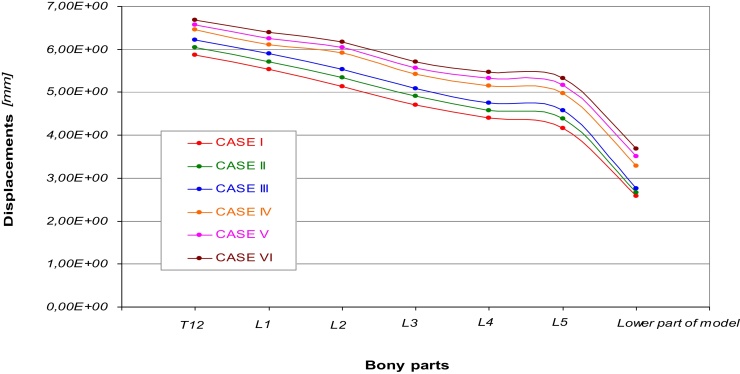
In Fig. 2 are reported the curves of displacements obtained in each part of the skeletal chain for all the six cases considered. Displacements exhibit a decreasing trend ranging from T12 to the lower part of the model. It is possible to evidence a correspondence of values for the curves referred to the cases I, II, and III, and the curves of the cases IV, V, and VI. In a general way it is possible to notice a plateau area located at L3, L4, and L5. On the lower part of the models all the first three cases show a displacement of about 2,6 mm, while in the other ones displacements range from 3,28 to 3,69 mm, see Table 3.
Fig. 2.
Displacements vs. different parts of the models referred to the six cases considered.
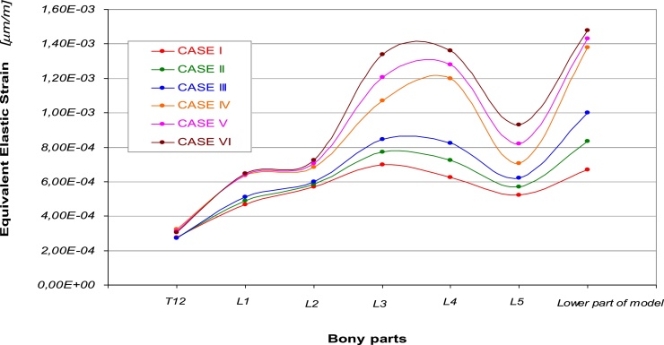
The six curves of the equivalent elastic strain, see Fig. 3, show a similar behavior obtained for the curves belonging to the first three cases, and an increasing trend evidenced by the other curves. In a general way all the six curves register higher values of equivalent elastic strain from T12 to L1, and a following decreasing of strain located at L2. Subsequently higher values of strain are reached by the curves related to the IV, V, VI cases in the L3 and L4 areas. This could mean that a different mechanism of strain shielding has been arranged inside the skeletal chain due to the particular geometrical configuration of the bony part imposed. At the L5 vertebra all the six curves present the minimum value of the equivalent elastic strain, while in the lower part of the model is located the maximum value, except for the case I which has its higher value of strain at the L3, see Table 3. The I, II, III cases show values ranging from 6,71E-04 to 1,00E-03 [μmm/mm], while for IV, V, and VI cases the obtained values are about 1,43E-03 [μmm/mm].
Fig. 3.
Equivalent elastic strain vs. different parts of the models referred to the six cases.
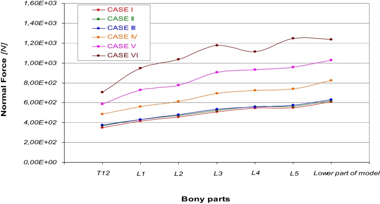
Fig. 4 depicts normal forces calculated in each bony part for the six cases. Also in this graph it is possible to notice a similar behavior showed by curves belonging to the first three cases which exhibit a general increasing trend and similar values of forces applied to the different bony parts. In order to confirm what already described for elastic strain, a different loading mechanism of bones, the other three curves (cases IV, V, VI) have always higher values of normal forces applied to the different parts of the bony chain considering successively IV, V, and VI cases. It is possible to notice in Case IV a decreasing trend located at L4.
Fig. 4.
Normal force vs. different parts of the models referred to the six cases.
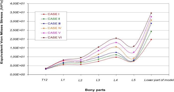
In Fig. 5 are reported the six curves of the equivalent Von Mises stress calculated for each bony part. In a general way they show always an increasing trend with the higher values of stress, 1,98E+01 MPa for Case I and 3,46E+01 MPa for case VI, reached in the lower part of the model. As it is possible to notice, in L5 all the six curves present a decreasing trend.
Fig. 5.
Equivalent Von Mises Stress vs. different parts of the models referred to the six cases.
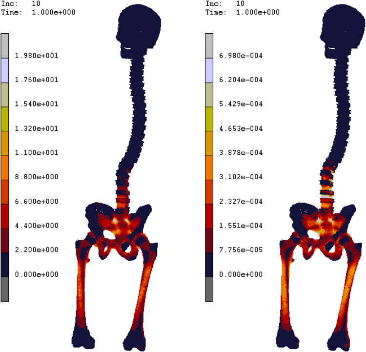
Finally in Fig. 6 are reported the equivalent elastic strain and equivalent Von Mises contour maps obtained for case I, results confirm higher values of stress and strain located at the pelvis and around the L3, L4 areas.
Fig. 6.
Equivalent Von Mises and equivalent elastic strain contour maps obtained for CASE I.
4. Discussion
Results obtained in this paper confirm a worsening of solicitation suffered by the bony parts going away from Case I to Case VI of Roussoly's classification. In particular way, first three cases seem to supply the different loading configurations spreading stresses in almost all the bony parts of the column, while the remaining others three cases produce an higher concentration of stress around the lower part of spline (L3, L4, L5).
Results confirm a good agreement with those present in litterature. An equivalent Von Mises average stress was of 0,55 MPa was found on the intervertebral disks with the higher values reached on the lower part of the column, in a good agreement with Miller et al., 1988.12 A comparison of our results, obtained for case I, with the ones found by Galbusera et al.,13 and El Rich et al.,14 obtained for a simulation of the physiological and balanced spine in the standing position, can be resumed in Table 4. As it is possible to notice our results in terms of normal compressive force are in good agreement with those of literature, a maximum error of −10% was evidenced with results found by Galbusera et al. In a general way our results confirm higher values of the compressive normal force soliciting the different bony parts. Different consideration can be argued by analyzing results concerning shear force, which confirm a good agreement with results obtained by El Rich et al., and a maximum error of −13%, but evident differences with Galbusera et al., maximum error of −97%, in a special way around areas of L3 and L4. Also in this case results are generally higher than literature. Finally also the values obtained for Sagittal moments are in good agreement with El Rich et al., maximum error +- 17%, while higher error percentage have been calculated in comparison with results obtained by Gaslbusera et al.
Table 4.
Comparison of Normal compressive force, Shear force, and sagittal moment (M − positive in extention) among our current model (CASE I) and literature data.
| El Rich et al. (2004) | Error | Galbusera et al. (2014) | Error | Current | |
|---|---|---|---|---|---|
| Normal Force [N] | |||||
| T12 | 3,36E+02 | (−4%) | \ | \ | 3,50E+02 |
| L1 | 4,03E+02 | (−3%) | 4,26E++02 | (+2%) | 4,16E+02 |
| L2 | 4,45E+02 | (−2%) | 4,40E+02 | (−3%) | 4,55E+02 |
| L3 | 4,97E+02 | (−3%) | 4,57E+02 | (−10%) | 5,10E+02 |
| L4 | 5,34E+02 | (−2%) | 5,08E+02 | (−7%) | 5,47E+02 |
| L5 | 5,75E+02 | (+4%) | 5,50E+02 | (0%) | 5,51E+02 |
| Shear Force [N] | |||||
| T12 | −3,80E+01 | (+9%) | \ | \ | −3,50E+01 |
| L1 | −5,10E+01 | (−2%) | −4,50E+01 | (−13%) | −5,20E+01 |
| L2 | −7,10E+01 | (−6%) | −5,00E+01 | (−34%) | −7,58E+01 |
| L3 | −9,00E+00 | (−12%) | −1,50E+01 | (+47%) | −1,02E+01 |
| L4 | 3,10E+01 | (−4%) | 1,00E+00 | (−97%) | 3,22E+01 |
| L5 | 2,18E+02 | (−13%) | 1,85E+02 | (−26%) | 2,50E+02 |
| Moment [N m] | |||||
| T12 | −8,30E+00 | (−5%) | \ | \ | −8,75E+00 |
| L1 | −6,30E+00 | (−9%) | −5,00E+00 | (−28%) | −6,93E+00 |
| L2 | −3,90E+00 | (−14%) | −2,90E+00 | (−36%) | −4,55E+00 |
| L3 | −1,50E+00 | (+17%) | −7,00E−01 | (−45%) | −1,28E+00 |
| L4 | −1,30E+00 | (−10%) | −7,00E−01 | (−51%) | −1,44E+00 |
| L5 | −2,30E+00 | (+17%) | −2,00E+00 | (+2%) | −1,97E+00 |
The results underline a relationship between PI increase, and accordingly of PT and LL, and the distribution of load forces. Load forces is exerted mainly on distal vertebrae, especially on L4 and L5. This result is in line with some papers in recent literature. Sahin et al.15 analyzed the medialization and tropism of lumbar vertebrae articular surfaces, pointing out that this event occurs previously and worsen fastly with higher PI values; however medialization and tropism can be observed along ageing. From 2,5 to 3% of the loading forces are usually distributed on the vertebrae posterior arch, they weigh on directly on articular apophysis, this percentages vary substantially accordingly to variations of spino-pelvic parameters. When Higher values of loads are reached vertebrae usually go ipertrophic and get a medialization of articular surfaces as a balance mechanism. Kalichman et al.16 found a direct relationship between medialization of articular surfaces and osteoarthrosis development on the same vertebrae. This makes the subject suitable for foraminal or central stenosis. Jentcshs et al.17 underlined that PI and FJ were related: the key point was identified about at 50°; this resulti s fitted with our model.
Recently, a correlation between high values of PI and Osteoarthrosis of the hip has been hyphotesized. Gabharth et al.,18 analyzing 400 well managed cadavers, have found pronounced arthrosis on those cadavers with high PI values (about 46.1). Hashimoto et al.19 have been found the same correlation even if their sample included subject with hip spine syndrome (lumbar back pain and coxofemoral pain. Even in this instance our results seem to corroborate this thesis. Moreover, Radcliff et Al. underlined a connection between high PI values and a very sagittal orientation of the acetabulum. This particular morphology, probably due to different load forces to which pelvis is subjected during growth, seems to be a predictive feature of a premature OA development. In addiction this feature has to be considered during total hip arthroplasty surgical planning: if it isn’t properly milled it may leave prothesis exposed.20
Conflict of interest
The authors have none to declare.
Author contributions
Study Concept and Desing: G. Cacciola, V. Filardi.
Acquisition of Data: S. Bertino, D. Milardi.
Analysis and interpretation of data: C. Caradonna, S. Portaro.
Drafting of Manuscript: G. Cacciola, S. Bertino, V. Filardi.
Critical Revision: A. Pisani, A. Barbanera.
References
- 1.Kardong . 6th ed. McGrawh-Hill; New York: 2012. Vertebrates: comparative anatomy, function, evolution. [Google Scholar]
- 2.4th ed. Elsevier.; 2016. Benzel’s spine surgery. [Google Scholar]
- 3.Hutchinson JR, http://link.springer.com/article/10.1007%2Fs00114-008-0488-3.
- 4.Le Huec J.C., Saddiki R., Franke J. Equilibrium of the human body and the gravity line: the basics. Eur Spine J. 2011;20:558. doi: 10.1007/s00586-011-1939-7. [DOI] [PMC free article] [PubMed] [Google Scholar]
- 5.Hogervorst Tom, Vereecke Evie E. Evolution of the human hip. Part 1: the osseous framework. J Hip Preserv Surg. 2014;1(2):39–45. doi: 10.1093/jhps/hnu013. [DOI] [PMC free article] [PubMed] [Google Scholar]
- 6.Hogervorst Tom, Vereecke Evie E. Evolution of the human hip. Part 1: muscling the double extension. J Hip Preserv Surg. 2015;2(1):3–14. doi: 10.1093/jhps/hnu014. [DOI] [PMC free article] [PubMed] [Google Scholar]
- 7.Vaz G., Roussouly P., Berthonnaud E., Dimnet J. Sagittal morphology and equilibrium of pelvis and spine. Eur Spine J. 2002;11(1):80–87. doi: 10.1007/s005860000224. [DOI] [PMC free article] [PubMed] [Google Scholar]
- 8.Roussouly Gollogly S., Berthonnaud E., Dimnet J. Classification of the normal variation in the sagittal alignment of the human lumbar spine and pelvis in the standing position. Spine (Phila Pa 1976) 2005;30(3):346–353. doi: 10.1097/01.brs.0000152379.54463.65. [DOI] [PubMed] [Google Scholar]
- 9.Daniel M. Role of optimization criterion in static asymmetric analysis of lumbar spine load? Wien Med Wochenschr. 2011;161(19–20):477–485. doi: 10.1007/s10354-011-0904-8. [DOI] [PubMed] [Google Scholar]
- 10.Filardi V. Stress shielding in the bony chain of leg in presence of varus or valgus knee. J Orthop. 2015;12(2):102–110. doi: 10.1016/j.jor.2014.06.007. [DOI] [PMC free article] [PubMed] [Google Scholar]
- 11.Filardi V. FE analysis of stress and displacements occurring in the bony chain of leg. J Orthop. 2014;11(4):157–165. doi: 10.1016/j.jor.2014.08.008. [DOI] [PMC free article] [PubMed] [Google Scholar]
- 12.Miller J.A., Schmatz C., Schultz A.B. Lumbar Disc Degeneration: correlation with age, sex and spine level in 600 autopsy specimen. Spine (Phila Pa 1976) 1988;13(2):173–178. [PubMed] [Google Scholar]
- 13.Galbusera F., Brayda-Bruno M., Costa F., Wilke H.J. Numerical evaluation of the correlation between the normal variation in the sagittal alignment of the lumbar spine and the spinal loads. J Orthop Res. 2014;32(4):537–544. doi: 10.1002/jor.22569. [DOI] [PubMed] [Google Scholar]
- 14.El-Rich M., Shirazi-Adl A., Arjmand N. Muscle activity, internal loads, and stability of the human spine in standing postures: combined model and in vivo studies. Spine (Phila Pa 1976) 2004;29(23):2633–2642. doi: 10.1097/01.brs.0000146463.05288.0e. [DOI] [PubMed] [Google Scholar]
- 15.Sahin M.S., Ergün A., Aslan A. The relationship between osteoarthritis of the lumbar facet joints and lumbosacropelvic morphology. Spine (Phila Pa 1976) 2015;40(19):E1058–62. doi: 10.1097/BRS.0000000000001070. [DOI] [PubMed] [Google Scholar]
- 16.Kalichman L., Suri P., Guermazi A., Li L., Hunter D.J. Facet orientation and tropism: associations with facet joint osteoarthritis and degeneratives. Spine (Phila Pa 1976) 2009;34(16):E579–E585. doi: 10.1097/BRS.0b013e3181aa2acb. [DOI] [PMC free article] [PubMed] [Google Scholar]
- 17.Jentzsch T., Geiger J., Bouaicha S., Slankamenac K., Nguyen-Kim T.D., Werner C.M. Increased pelvic incidence may lead to arthritis and sagittal orientation of the facet joints at the lower lumbar spine. BMC Med Imaging. 2013;5(13):34. doi: 10.1186/1471-2342-13-34. [DOI] [PMC free article] [PubMed] [Google Scholar]
- 18.Gebhart J.J., Weinberg D.S., Bohl M.S., Liu R.W. Relationship between pelvic incidence and osteoarthritis of the hip. Bone Jt Res. 2016;5(2):66–72. doi: 10.1302/2046-3758.52.2000552. [DOI] [PMC free article] [PubMed] [Google Scholar]
- 19.Hashimoto S., Fujishiro T., Hayashi S., Kanzaki N., Nishiyama T., Kurosaka M. Clinical importance of impingement deformities for hip osteoarthritis progression in a Japanese population. Int Orthop. 2014;38(8):1609–1614. doi: 10.1007/s00264-014-2393-z. [DOI] [PMC free article] [PubMed] [Google Scholar]
- 20.Radcliff K.E., Kepler C.K., Hellman M. Does spinal alignment influence acetabular orientation: a study of spinopelvic variables and sagittal acetabular version. Orthop Surg. 2014;6(1):15–22. doi: 10.1111/os.12090. [DOI] [PMC free article] [PubMed] [Google Scholar]


