Modeling Shift-Variant X-Ray Focal Spot Blur for High-Resolution Flat-Panel Cone-Beam CT

Abstract

Flat-panel cone-beam CT (CBCT) has been applied clinically in a number of high-resolution applications. Increasing geometric magnification can potentially improve resolution, but also increases blur due to an extended x-ray focal-spot. We present a shift-variant focal-spot blur model and incorporate it into a model-based iterative-reconstruction algorithm. We apply this algorithm to simulation and CBCT test-bench data. In a trabecular bone simulation study, we find traditional reconstruction approaches without a blur model exhibit shift-variant resolution properties that depend greatly on the acquisition protocol (e.g. short vs. full scans) and the anode angles of the rays used to reconstruct a particular region. For physical CBCT experiments focal spot blur was characterized and a spatial resolution phantom was scanned and reconstructed. In both experiments image quality using the shift-variant model was significantly improved over approaches that modeled no blur or only a shift-invariant blur, suggesting a potential means to overcome traditional CBCT spatial resolution and system design limitations.

I. Introduction

Flat-panel cone-beam CT (CBCT) is a promising modality for high-resolution applications, such as quantitative trabecular bone analysis in extremities imaging and microcalcification detection in mammography. Current application-specific imaging systems are often unable to resolve all trabeculae or microcalcifications, which can be on the order of 100μm. A high-magnification geometry has the potential to improve resolution, but projections suffer from increased blur due to the extended focal spot. Model-based iterative reconstruction (MBIR) methods have previously demonstrated improved image quality through the use of sophisticated system and noise models. Proper modeling of the x-ray focal spot, and incorporation of this model into a MBIR method, can mitigate the effects of focal spot blur in high-resolution high-magnification reconstructions.

Previously, we have developed a reconstruction method that models detector blur, focal spot blur, and spatial noise correlations using a staged approach (deblurring and other preprocessing followed by reconstruction).[1] Shift-invariant blur models were assumed in order to simplify deblurring. However, such assumptions are not valid at large fan angles, where the angulation of the anode results in a position-dependent apparent focal-spot shape. Moreover, this effect is more pronounced in high-magnification systems due to a larger focal-spot blur. Properly modeling shift-variant focal-spot blur is critical to generating high-resolution images in these systems. Previous work by La Rivière to model shift-variant focal-spot blur addressed deblurring data for multidetector CT systems with the anode-cathode axis of the x-ray source oriented axially.[2]

In this work, we characterize focal spot blur along the anode-cathode axis in a CBCT system where this axis is perpendicular to the axis of rotation (a common orientation in CBCT systems). We use a non-linear objective function that includes shift-variant blur in the forward model (e.g. no deblurring in preprocessing) to reconstruct high-resolution objects in simulation and test-bench studies.

II. Methods

A. Forward Model and Objective Function

We use the general forward model:

$$y~\mathcal{N}(\mathbf{B}exp(-\mathbf{A}\mu ),{\mathbf{K}}_Y)$$ (1)

with measurement vector, y, and object attenuation values, μ. The linear operator B contains focal spot blur and gain terms (e.g. photons per pixel), A is the forward projector, and K_Y is the measurement covariance matrix. The corresponding penalized-likelihood objective function is:

$$\widehat{\mu }=argmin{\Vert y-\mathbf{B}exp(-\mathbf{A}\mu )\Vert }_{{\mathbf{K}}_Y^{-1}}^2+\beta R(\mu )$$ (2)

where R is a penalty function and β is the penalty strength.

Equation (2) was minimized using a separable paraboloid surrogates approach, similar to that of Erdoğan et al.[3], [4] but with an added separability step in the B exp(−Aμ) term. The resulting baseline algorithm is:

$a={\mathbf{B}}^T{\mathbf{K}}_Y^{-1}\mathbf{B}1$, γ = A1, $b=\mathbf{B}{\mathbf{K}}_Y^{-1}y$

for n = 1 : N do

l(n) = Aμ(n)

$d^{(n)}=-b-\mathbf{D}\{a\}exp(-l^{(n)})+{\mathbf{B}}^T{\mathbf{K}}_Y^{-1}\mathbf{B}exp(-l^{(n)})$

$h_j^{(n)}(l_j)\triangleq 0.5a_{j}exp(-2l_j)+exp(-l_j)d_j^{(n)}$

$c_j^{(n)}=\text{optimum}\text{curvature}\text{of}{h}_j^{(n)}$ from [3]

L(n) = AT(−D{a}exp(−2l(n)) − D{dn}exp(−l(n)))

$c_{\mu }^{(n)}={\mathbf{A}}^T\mathbf{D}\{\gamma \}{c}^{(n)}$

${\mu }^{(n+1)}={\left[{\mu }^{(n)}+\frac{-L^{(n)}-\beta \nabla R{\mid }_{{\mu }^{(n)}}}{c_{\mu }^{(n)}+\beta {\nabla }^{2}R{\mid }_{{\mu }^{(n)}}}\right]}_{+}$

end for

We further extend the algorithm using Nesterov’s acceleration method. All reconstructions used 20 ordered subsets.[4] The regularization gradient and curvature were computed using standard surrogate techniques.[4]

B. Shift-Variant Blur Model

We model the shift-variant focal spot blur along directions parallel to the detector. The model approximates a depth-independent blur. (See § IV for a discussion of depth-dependent effects.) Therefore, the blur model can be included in the B term in (1). To estimate a continuous source-blur model for discrete inputs and outputs, we use nearest neighbor interpolation to create a continous approximation of the input image, apply a convolution operation, then discretize the signal using a rectangular kernel with the dimensions of a pixel and sampling at pixel centers. The full operation is:

$$g[k,l]={\int }_{x,y}{\int }_{\xi ,\eta }\sum _{i,j}f\left[i,j\right]\text{rect}(\frac{\xi -i{T}_x}{T_x},\frac{\eta -j{T}_y}{T_y})T_x{T}_{y}h(x,y;\xi ,\eta )\text{rect}(\frac{x-l{T}_x}{T_x},\frac{y-k{T}_y}{T_y})d\xi d\eta dxdy$$ (3)

where f and g are the input and output images, T_x and T_y are the pixel widths along the corresponding directions and h(·, ·; ξ, η) is the impulse response of a point source at ξ, η. Equation (3) can be approximated by discretizing variables and assuming h is constant over small displacements. We sample x and ξ at intervals of T_x/s and y and η at intervals of T_y/s, where s is an odd integer. Applying these approximations and simplifying leads to:

$$g[k,l]\approx \sum _{j,i,a,b}f[i,j]\mid 1-a\Vert 1-b\mid h((a+l)T_x,(b+k)T_y;i{T}_x,j{T}_y)T_x{T}_y/s^2$$ (4)

where a and b range from −(s − 1)/s to (s − 1)/s in increments of 1/s. The transpose operation (e.g. for B^T) requires switching the indices for f and g, and summing over k, l instead of i, j.

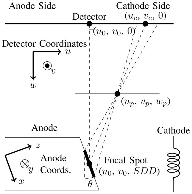
The impulse response (h) centered at a given point (u_c, v_c) is assumed to be a binary function, with values either equal to 0 or k = area(h(·, ·; u_c, v_c))⁻¹. To determine the value of h(u, v; u_c, v_c), the point (u, v) is backprojected through a pinhole onto the anode. A two dimensional cross section of the geometry is illustrated in Figure 1. The pinhole is placed a distance w_p from the detector and along the line connecting (u_c, v_c) with the center of the focal spot. If the backprojected point is in the rectangular focal spot, h(u, v; u_c, v_c) = k, otherwise h(u, v; u_c, v_c) = 0. The area of h was found by forward projecting the corners of the focal spot through the pinhole, and applying Bretschneider’s formula to the resulting points.[5]

Fig. 1.

Geometry used to calculate the focal spot blur impulse response. The focal spot is represented by the bold line on the side of the anode. All coordinates are in detector coordinates. The origin of the anode coordinate system is at (u₀, v₀, SDD).

C. Simulation Study

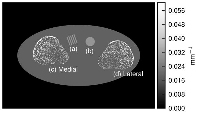
Data were generated from the digital extremities phantom in Figure 2. Line integrals were generated from a high-resolution truth image (3300×2300 image of 30μm voxels) projected onto a one-dimensional detector with 8192 pixels and a 48.5μm pixel pitch. A high-magnification geometry was used, with a source-detector distance of 1200mm, a source-axis distance of 250mm, and an angular spacing of 0.5°. These line integrals were downsampled by a factor of 4 to give a pixel pitch of 194μm. Measurements were generated from the downsampled line integrals (l) according to:

$$y_{\text{noiseless}}={\mathbf{B}}_s{I}_{0}exp(-l)$$ (5)

$$y=y_{\text{noiseless}}+\mathcal{N}(0,\mathbf{D}\{y_{\text{noiseless}}\})+\mathcal{N}(0,\mathbf{D}\{{\sigma }_{ro}^2\})$$ (6)

where I₀ is 10⁴ photons per pixel, B_s is the focal spot blur operator (we assume there is no detector blur), and the readout-noise standard deviation (σ_ro) is 3.32 photons. The focal spot was modeled as a 5mm×0.8mm rectangle on a 14° anode with the anode-cathode axis parallel to the detector row. The sampling factor (s) was equal to 41. (Note that B_sI₀ is equivalent to B in (1).) Data were generated using two short scans (short-1 and short-2) spaced 180 degrees apart, and a full scan. The short-1 scan placed the medial bone (Figure 2c) predominately on the anode side, and the lateral bone (2d) predominately on the cathode side. The reverse is true for the short-2 scan.

Fig. 2.

Digital extremeties phantom with medial (c) and lateral (d) bones, line pairs (a), and a uniform disc (b).

Data from each scan were reconstructed using the algorithm presented above with three models for focal-spot blur: identity (no blur), shift-invariant blur, and shift-variant blur. The sampling factor (s) used in reconstructions was 11. Data were reconstructed into a 1650×1150 volume of 60μm voxels using a Huber penalty (δ = 10⁻⁴). The covariance matrix was modeled as $\mathbf{D}\{y+{\sigma }_{ro}^2\}$.

The accuracy of trabeculae segmentation in the medial and lateral bones was used as a measure of image quality. The truth segmentation for each bone was found by downsampling the high-resolution phantom to match the reconstruction volume dimensions and thresholding at the average attenuation of bone and fat. Data were reconstructed at several penalty strengths and thresholded at regularly spaced values between the attenuation values of fat and bone. Accuracy was quantified as the mutual overlap between the thresholded truth, t, and the thresholded reconstruction, r:[6]

$$\text{mutual}\text{overlap}(t,r)=2(\sum tr){(\sum (t+r))}^{-1}$$ (7)

D. Bench Characterization

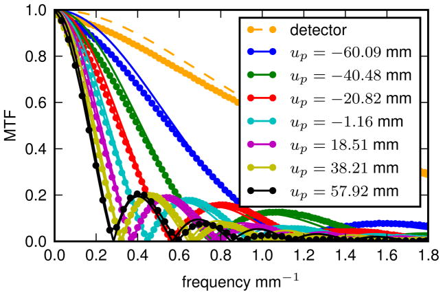
To apply the approach to physical data, we characterized the focal spot blur on a CBCT test bench consisting of a Rad-94 x-ray tube (Varian, Salt Lake City UT), a PaxScan 4343CB flat-panel detector (Varian, Palo Alto CA), and a SDD of 108 cm. In this work we focus on two-dimensional reconstructions, and therefore only measure one dimensional MTFs along the u axis. MTFs were measured using a tungsten edge[1][7] placed at isocenter (40cm from the source) and translated in the ±u directions. The detector MTF was measured by placing the edge at the detector. We assume the detector MTF is shift-invariant and fit it to the following model:[8]

$$\mid {\mathit{MTF}}_d(f_u)\mid =\left|\frac{\text{sinc}(f_u{T}_x)}{1+H{f}_u^2}\right|$$ (8)

where f_u is the spatial frequency in mm⁻¹ and H is a blur parameter. The focal spot MTF at each position u_p was modeled as a rect function with an apparent length L(u_p), resulting in the combined MTF:

$$\mid {\mathit{MTF}}_{sd}\mid (f_u;u_p)=\mid \text{sinc}(f_{u}L(u_p)){\mathit{MTF}}_d(f_u)\mid$$ (9)

Theoretical apparent blur lengths from anode angle (θ) and focal spot length (L) were fit to the measured lengths to yield estimates for θ and L.

E. Resolution Phantom Study

A cylindrical resolution phantom (CatPhan CTP528 High Resolution Module, Phantom Laboratory, Salem, NY) with variable frequency line pairs was scanned on the CBCT test bench. The source-detector and source-axis distances were 108 cm and 40 cm respectively. A full scan of 720 projections was collected at 80 kVp and 0.504 mAs per projection. Data were reconstructed using the identity and shift-variant blur models, as well as three shift-invariant blur models. The three shift-invariant blurs modeled were the blur at the center of the detector (as in the simulation study) and the blur at either edge of the detector. The presented MBIR algorithm was used with 800 iterations to ensure a nearly converged solution. The reconstruction volume was 170mm×170mm with 100μm voxels. The blur model used the focal spot length and anode angle from § II-D and a subset parameter (s) of 5. We assume that detector blur is negligible and do not model it in the reconstruction algorithm.

III. Results

A. Simulation Study

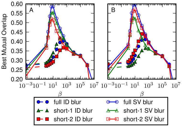
The best mutual overlap values (over all threshold values) for each (β) are shown in Figure 3. Results are shown for reconstructions with an identity (ID) blur model and the shift-variant (SV) blur model. Each line represents a blur model and scan type combination, and each point represents a reconstruction. A higher best mutual overlap indicates that a segmentation based on that reconstruction is closer to the truth segmentation, and the reconstruction is therefore more accurate. All methods that used the SV model were more accurate than those that used the ID model, which is evident by comparing the maximum of each line. With the ID model, the best quality segmentation of the medial bone is achieved with data from the short-1 scan, which placed the medial bone projections primarily on the high-resolution (anode) side of the detector. The lowest quality was the short-2 scan, which placed the projections primarily on the low-resolution (cathode) side. The full scan reconstructions with the ID model rank between the reconstructions from the two short scans. Neglecting to model blur is equivalent to assuming that classically redundant projections in the full scan (i.e. those with the same integration path but reversed direction) contain the same information, despite the fact that they are subject to different degrees of blurring, which results in a reconstruction whose image quality is a compromise between that of the two short scan reconstructions. Predictably, the lateral bone reconstructions are best when using the short-2 scan and worst when using the short-1 scan, in which the lateral bone projection data was on the high- and low-resolution sides of the detector, respectively.

Fig. 3.

Best mutual overlap versus β. A) Medial and B) Lateral bone.

When using the SV model, the full scan provides the best reconstruction of both bones, followed by the short-1 scan and then the short-2 scan in the case of the medial bone, and the short-2 scan and then the short-1 scan for the lateral bone. The better image quality of the full scan images over the corresponding high-resolution short-scan reconstructions can be attributed to the additional (low-resolution) data. The SV model can use this additional information to improve the reconstruction without losing details provided by the high-resolution data. In effect, rather than averaging the redundant data, the low-frequency data is used to reduce noise while the high-frequency data maintains spatial resolution. The corresponding low-resolution scan for each bone (short-2 for the medial bone and short-1 for the lateral bone) results in the lowest quality reconstructions due to the increased difficulty in deblurring the data.

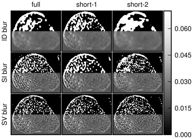
Figure 4 shows the medial-bone reconstructions (bottom of each image) and segmentations (top of each image) corresponding to the best possible mutual overlap (optimal threshold and β values) with each scan type and blur model combination. All SV reconstructions depict more trabecular structure than the shift-invariant (SI) or ID models. The difference in image quality among ID reconstructions is readily apparent in these images, with the short-1 scan resulting in the most trabecular detail. Finally, the SI images depict more detail than the ID model but less detail than the SV reconstructions. However, the SI model results in a ringing artifact, particularly evident on the lower left aspect of the medial bone in the full scan reconstruction. This is likely due to blur/model mismatch (the SI model is accurate at the center of the detector but less accurate at the edges).

Fig. 4.

Reconstructions of the medial bone with the highest mutual overlap over all thresholds and β’s. The top half of each reconstruction is thresholded.

B. Focal Spot Measurement

The detector MTF and the combined focal-spot and detector MTFs at different positions are shown in Figure 5. The magnification in this system was about 2.7, so that the focal-spot blur dominates over the detector blur. Each combined focal-spot and detector MTF is labeled by the distance of the tungsten edge from the central ray. At positive positions, the edge is on the cathode side, and at negative positions the edge is on the anode side. There is a dramatic difference in MTFs at different positions due to the angulation of the anode. Fits for each MTF are also shown. These fits give the apparent length of the focal spot at each position, which was used to estimate the actual length of the focal spot and the angle of the anode. The focal spot length was found to be 5.23mm and the anode angle was 14.3°.

Fig. 5.

MTFs and fits for the detector and the detector+source blur at different displacements from the center of rotation.

C. Bench Study

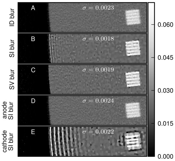
Figure 6 shows the same region-of-interest of five reconstructions, each of which used a different blur model. The three SI blur models are the apparent focal spot size at the center, anode side, and cathode side of the detector. The reconstructions have approximately the same amount of noise (estimated by computing standard deviation in a flat region at the center of the phantom). The line pairs in the SV (6c) and center SI (6b) reconstructions are much sharper than those in the ID reconstruction (6a). That the SI reconstruction line-pairs are roughly as sharp as those of the SV reconstruction suggests that at this distance from isocenter (approximately 4.75cm) the SI approximation is fairly accurate. However, at the edge of the phantom (approximately 7.5cm from isocenter), this assumption breaks down, and the resulting mismatch between the model and the actual blur results in a “ringing” artifact. The anode-side SI blur model (6d) underestimates the blur over most of the detector, reducing ringing compared to the center SI blur model but also reducing the sharpness of the line pairs. The cathode-side SI blur model (6e) overestimates the blur over much of the detector, increasing the ringing artifact.

Fig. 6.

Physical CBCT reconstructions. Each subfigure shows a portion of the phantom from the edge to one of the line pairs. Each reconstruction has approximately the same noise level (indicated in each subplot in units of mm⁻¹ and denoted by σ).

IV. Discussion

The image quality difference in identity blur model reconstructions from the two different short scans illustrates the importance of considering shift-variance in high-resolution, high-magnification systems. The poor image quality and/or ringing artifact in the reconstructions with a shift-invariant blur model demonstrate that this model is a poor approximation for large objects (relative to the field of view), and that a full shift-variant model is more appropriate. These results also suggest a means to improve local resolution properties when advanced blur models are not available: if the location of a high resolution target in the object is known a priori, then that object can be placed such that the high resolution target favors the anode side of the detector during a short scan.

This work suggests x-ray tube orientation is an important factor in system design. Blur shift-variance, and therefore reconstruction resolution, will depend on whether the anode-cathode axis is oriented parallel or perpendicular to the axis of rotation. Models such as the one presented may alter the trade-off associated with tube orientation, allowing for more flexibility in system design. Future studies will analyze three-dimensional reconstructions in order to properly characterize resolution/image quality both in-plane and axially. While we have demonstrated the utility of a depth-independent source blur model, future work will consider depth-dependent source blur effects. In the presented bench study, we estimate that apparent focal spot size approximately doubled over the length of the object along the source-detector direction. By comparison, the measured apparent focal-spot lengths approximately quadrupled over the length the object along the direction parallel to the detector. Thus, depth-dependent shift-variance is a large effect, but not as large as shift-variance due to anode angulation.

We have provided a method to improve image quality with an advanced shift-variant blur model, and used this model to reconstruct high-resolution trabecular details in a simulation study and fine line-pair patterns on a CBCT test bench. This technique could help overcome spatial resolution limits in high-magnification systems, improving current systems and allowing new systems to be designed with higher magnifications for high-resolution applications.

References

- 1.Tilley S, II, et al. Model-based iterative reconstruction for flat-panel cone-beam CT with focal spot blur, detector blur, and correlated noise. Physics in Medicine and Biology. 2016;61(1) doi: 10.1088/0031-9155/61/1/296. [DOI] [PMC free article] [PubMed] [Google Scholar]
- 2.La Rivière PJ, et al. Correction for resolution nonuniformities caused by anode angulation in computed tomography. IEEE transactions on medical imaging. 2008;27(9) doi: 10.1109/TMI.2008.923639. [DOI] [PMC free article] [PubMed] [Google Scholar]
- 3.Erdoğan H, et al. Monotonic algorithms for transmission tomography. IEEE transactions on medical imaging. 1999 Sep;18(9) doi: 10.1109/42.802758. [DOI] [PubMed] [Google Scholar]
- 4.Erdoğan H, et al. Ordered subsets algorithms for transmission tomography. Physics in medicine and biology. 1999;2835 doi: 10.1088/0031-9155/44/11/311. [DOI] [PubMed] [Google Scholar]
- 5.Weisstein EW. Bretschneider’s Formula. http://mathworld.wolfram.com/BretschneidersFormula.html.
- 6.Sonka M, et al. ISE Image Processing, Analysis and Machine Vision. Nelson Engineering; Apr, 2007. Chapter 6: Segmentation 1. student ed edition ed. [Google Scholar]
- 7.Samei E, et al. A method for measuring the presampled MTF of digital radiographic systems using an edge test device. Medical Physics. 1998;25(1) doi: 10.1118/1.598165. [DOI] [PubMed] [Google Scholar]
- 8.Siewerdsen JH, et al. Signal, noise power spectrum, and detective quantum efficiency of indirect-detection flat-panel imagers for diagnostic radiology. Medical Physics. 1998 May;25(5) doi: 10.1118/1.598243. [DOI] [PubMed] [Google Scholar]