Spatially-dependent Bayesian model selection for disease mapping

Abstract

In disease mapping where predictor effects are to be modeled, it is often the case that sets of predictors are fixed, and the aim is to choose between fixed model sets. Model selection methods, both Bayesian model selection and Bayesian model averaging, are approaches within the Bayesian paradigm for achieving this aim. In the spatial context, model selection could have a spatial component in the sense that some models may be more appropriate for certain areas of a study region than others. In this work, we examine the use of spatially referenced Bayesian model averaging and Bayesian model selection via a large-scale simulation study accompanied by a small-scale case study. Our results suggest that BMS performs well when a strong regression signature is found.

1 Introduction

There are many instances in the disease mapping framework where one may wish to select between two or more linear predictors, or models, of interest. In certain situations, the model selection process may be more applicable than simply using variable selection; for example, if there are prior beliefs that these particular linear predictors could be informative.

In this paper, we discuss a way to implement non-spatial and spatial Bayesian model selection (BMS) in comparison to Bayesian model averaging (BMA)^1–3 using the BUGS software BRugs and R2WinBUGS which call OpenBUGS and WinBUGS, respectively.^4,5 Both of these methods are considered to be model selection techniques and can be used in lieu of variable selection as they alleviate some of the issues related to variable selection (e.g. co-linearity).^6–11 Here, if two or more predictors are known to be collinear, we suggest that they should be included in different linear predictors that the method is selecting between. The structure of our proposed BMS procedure is similar to BMA, and thus this commonly used method can be compared.

There are several useful variable selection procedures available in the Bayesian paradigm,^12,13 but we believe that model selection is the better alternative, especially when there are particular linear predictors of interest. Similar comparisons between BMA and variable selection have been performed in the past. Viallefont’s simulation study first shows that variable selection methods often produce too many variables selected as ‘significant.’ Then, they determined that BMA produces easy to interpret, precise results displaying the posterior probability that a variable is a risk factor. They also caution users about interpreting the averaged posterior parameters as each of the alternative linear predictors has been adjusted for different confounders.¹⁴

Spatial model selection, which allows different linear predictors to be selected for each spatial unit, is the main focus of this paper. The data are partitioned into different spatial areas to determine how well the model selection procedures recover the truth when spatial structure is present in the data. We make a comparison of BMS to BMA, and additionally calculate goodness of fit (GoF) measures for each of the partitioned areas.

This paper is developed as follows. First, we describe the methods associated with the BMS and BMA processes. Next, we discuss the development of our simulated dataset and the different models used for exploring this methodology. Finally, we discuss the benefits of using the model selection method under different scenarios in the disease mapping context.

2 Methods

Our paper focuses on the context of disease mapping in m predefined small areas. We make the conventional assumption that an aggregate count of disease (y_i) is observed in the ith small area and that these outcome counts are conditionally independent Poisson distributed outcomes, i.e. y_i|μ_i~Pois(μ_i). This is a commonly assumed model for small area counts in disease mapping.¹⁵ In what follows, we examine two types of model formulation: complete and partial models. For the complete models, it is assumed that the linear predictor applies to the whole study region, in the sense that the underlying model is the same for all areas. In the partial models, it is assumed that the underlying linear predictor is different for different partitions of the set of spatial units.

2.1 Bayesian model selection

To evaluate a number of alternative linear predictor models, we can adopt a method which fits a variety of models, and the selection of weights allows each model to be evaluated for its appropriateness. In general, for d = 1, …, D complete models, the following structure applies

$$\begin{array}{c}{y}_i|{\mu }_i~\mathit{Poi}\left({\mu }_i\right)\\ {\mu }_i=e_i{\theta }_i\\ \log \left({\theta }_i\right)={\displaystyle \sum _d{w}_d{\phi }_{\mathit{id}}}\\ \log \mathrm{it}\left(p_d\right)~\mathit{Norm}\left(0,{\tau }_d\right)\\ w_d~\mathit{Bern}\left(p_d\right)\end{array}$$

where φ_id is our dth model’s suggested linear predictor complimented with possible random effects. In general, we write φ_id as $x_i^T\beta \psi +u_i{\psi }_{\mathrm{d},J+1}+v_i{\psi }_{\mathrm{d},J+2}$ with $x_i^T$, the vector of J possible covariates, j = 1, …, J + 2, u_i the uncorrelated heterogeneous (UH) term, v_i the correlated heterogeneous (CH) term, and ψ_dj an indicator for if the jth predictor or random effect is to be included in the linear predictor of the d^th model. Model priors here as well as in the following models are such that β_dj~Norm(0, 1), u_i Norm(0, τ_u), τ_u~Gam(1, 0.5), v_i~CAR(τ_v), τ_v~Gam(1, 0.5), and ${\tau }_d^{-1/2}~\mathit{Unif}\left(0,5\right)$. Hence, for a variable not included in dth the model, ψ_dj would be zero, otherwise it would be one. Further, w_d is a model selection indicator, equal to 1 if the dth model is selected and zero otherwise. The model selection probability is given by the probabilities p_d. For the partial models, the following structure applies

$$\begin{array}{c}{y}_i~\mathit{Poi}\left({\mu }_i\right)\\ {\mu }_i=e_i{\theta }_i\\ \log \left({\theta }_i\right)={\displaystyle \sum _d{w}_{id}{\phi }_{id}}\\ \log \mathrm{it}\left(p_{id}\right)~\mathit{Norm}\left(\frac{1}{n_i}{\displaystyle \sum _{i~l}\log \mathrm{it}\left(p_{\mathit{idl}}\right),\frac{1}{n_i{\tau }_{id}}}\right)\\ w_{id}~\mathit{Bern}\left(p_{id}\right)\end{array}$$

in which the model selection indicator is spatially structured. In the equations, i ≠ l, n_i is the number of neighbors for county i, and i ~ l indicates that the two counties i and l are neighbors. This is an intrinsic conditional autoregressive (CAR) model, which adds the desired spatial structure to the model selection process and a new level of complexity in comparison to the complete models.

2.2 Bayesian model averaging

BMA is similar to the BMS technique described in the previous section.² This method averages over the D possible models, M₁, …, M_D to find the posterior distribution of θ as follows

$$P\left(\theta |y_1,\dots ,y_m\right)={\displaystyle \sum _{d=1}^{D}P\left(\theta |y_1,\dots ,y_m,M_d\right)P\left(M_d|y_1,\dots ,y_m\right)}$$

where P(M_d|y₁, …, y_m) is the model probability for model d, and P(θ|y₁, …, y_m, M_d) is determined by marginalizing the posterior of the model parameters. The posterior probability for selection model M_d is given by^1,2,14

$$\begin{array}{l}P\left(M_d|y_1,\dots ,y_m\right)=P\left(y_1,\dots ,y_m|M_d\right)P\left(M_d\right)/C\\ \mathrm{where}C={\displaystyle \sum _{l=1}^{D}P\left(y_1,\dots ,y_m|M_l\right)P\left(M_l\right)}\\ \mathrm{and}P\left(y_1,\dots ,y_m|M_d\right)={\displaystyle \int P\left(y_1,\dots ,y_m|{\theta }_d,M_d\right)P\left({\theta }_d|M_l\right)\mathrm{d}{\theta }_d}\end{array}$$

Alternatively, we can estimate the model probabilities P(M_d|y₁, …, y_m) using the deviance information criteria (DIC). The model probabilities can be approximated by¹⁶

$$\begin{array}{c}{p}_{\mathit{DIC}1}\left(M_d|y_1,\dots ,y_m\right)\approx \frac{e^{-\mathit{DI}{C}_d}}{{\displaystyle {\sum }_k{e}^{-\mathit{DI}{C}_k}}}\\ p_{\mathit{DIC}2}\left(M_d|y_1,\dots ,y_m\right)\approx \frac{{\displaystyle {\sum }_i{e}^{-DI{C}_{id}}}}{{\displaystyle {\sum }_k{\displaystyle {\sum }_i{e}^{-DI{C}_{ik}}}}}\end{array}$$

In these expressions, DIC_d is the DIC associated with the d^th alternative linear predictor. Note that in the first expression, the DICs are calculated overall (over all areas), whereas in the second expression, the DICs are calculated locally (per region). We calculate this measure by collecting the deviance for each of the alternative linear predictors using the Poisson likelihood as follows

$$D_i\left({\theta }_i\right)=-2\left(l_i\left({\theta }_i\right)\right)=-2\left(y_i\log \left(e_i{\theta }_i\right)-e_i{\theta }_i-\log \left(y_i!\right)\right)$$

Next, $\overline{D_i}$ is computed from the sampler and supplied to the following function to calculate the local DIC for county i: ${\mathit{DIC}}_i=\overline{D_i}+p{D}_i$ where ${\mathit{pD}}_i=\overline{D_i}=D_i\left(\overline{\theta }\right)$ and ${\overline{\theta }}_i$ is posterior the mean of θ_i. Finally, the model DIC is simply the sum of the local DICs.

To apply the BMA framework to the partial models, we apply the same type of spatial structure seen with BMS on the model probabilities by way of the CAR model. Then, we simply use the local DIC to calculate the alternative model probabilities measure for each of the m areas.

3 Simulated data and fitted models

In this and the following sections, models will be referred to by the contents of both the simulated data and the fitted model applied. Table 1 is a list of notations for describing models, and Supplemental Table 1 is a list of all simulated data models explicitly defined.

Table 1.

Notation for describing model contents.

Notation	Definition
E1	Model with ei = 1
E2	Model with ei ~ Gam (1,1)
C	Complete model
P	Partial model
SX	Simulated data model ‘X’
FX	Fitted model ‘X’
RE	Model with an uncorrelated random effect included
CV	Model with a convolution component included

3.1 Simulated data

To evaluate the performance of these alternative approaches, we simulate data to establish realistic ground truth for disease risk variation. To match the methods described above, we define a count outcome as y_i in the ith small area. We assume a map of m small areas. In addition, we assume that the expected count (e_i) is available in each small area. Thus, our outcome follows a Poisson distribution with expectation μ_i in county i.

In the simulations, we fix the expected rate for the areas in order to focus on the estimation of relative risk θ_i. To complete the parameterization, we assume a relative risk which is parameterized with a range of different risk models.

We chose the county map of the state of Georgia, USA which has 159 areas (counties). Hence, i = (1, …, 159) for this county set. We consider two scenarios for the expected rates. In the first scenario, the expected rates e_i are assumed to be constant over all areas, and are set at 1. For the second scenario, the expected rates are assumed to be varying over the areas, and are assumed to be a realization of a Gam(1, 1) distribution. Having these two scenarios in the simulation study allows us to see how the extra variation affects the model selection processes. We denote this in our model names as E1 and E2 for fixed and varying expected rates, respectively.

We examined nine basic models for risk (S1 up to S9) which have different combinations of covariates and random effects as might be found in common applications. First, we generated four predictors with different spatial patterns. The four chosen variables were median age (x₁), median education (x₂), median income (x₃), and a binary predictor representing presence/absence of a major medical center in a county (x₄). These variables are county-level measures for the 159 counties in the state of Georgia. We chose these variables because it is important to represent a range of different spatial structures and types of predictors. Additionally, observed predictors/covariates could have a spatial structure, and thus we included this in the definition of two of the predictors (median age and major medical center). Table 2 displays the predictors generated via simulation and their parameterization where the Gaussian parameters are the mean and variance. Also, note that the spatial predictors have a covariance structure applied, but this is explained in detail later.

Table 2.

Description of predictor variables and their simulation marginal distribution.

Variable	Spatial	Distribution (marginal)
Median age (Years)	Yes	x1 ~ Norm (40,4)
Median education (Years)	No	x2 ~ Norm (13,4)
Median income (Thousands of Dollars)	No	x3 ~ Norm (45,1)
Major medical center (Yes/No)	Yes
		π ~ Norm(0,25)
		logit(p) = π
		x4 ~ Bern(p)

These distributions lead to measures that reflect typical values for these variables. For example, the median age for a county in the USA is roughly 40, and the values do not vary much from one county to the next. Similar explanations can be applied to both the median education and median income variables. For the major medical center variable, this indicated marginal distribution leads to roughly half of the counties answering ‘yes’ to having a major medical center. These variables have been selected as placeholders, and should be thought of as representing any of the typical variables one might utilize in building disease mapping models.

The spatially structured covariates were generated using the RandomFields package in R.¹⁷ The simulation uses the county centroid as a location to create a Gaussian Random Field (GRF), which is defined via a covariance structure. We assume a Gaussian covariance structure, and this assumption leads to a stationary and isotropic process.¹⁸ We specify this structure by using the RMgauss() command. We assume a power exponential covariance model of the form

$$C\left(r\right)=e^{-\alpha r^2}$$

where r is the Euclidean distance between two centroids and the covariance parameter (α) is set as α = 1. Following the selection of the covariance structure, we must also set the mean of the GRF to create the same marginal distributions as described in Table 2 using the RMtrend() command. Finally, to simulate the GRF, we use the RFsimulate() command to create a GRF and assign a value to the spatial covariate. There is only a slight extension that must be applied when the spatial covariate is binary such as x₄. To create this variable, we use a GRF to simulate π mentioned in Table 2, rather than the covariate itself. From there, we simulate from a Bernoulli distribution to give the binary indicators for each county, using expit(π) for the probabilities.

The distribution of all covariates, x₁, …, x₄, on the Georgia county map is illustrated in Figure 1. Notice that the median age and major medical center covariates appropriately appear to have spatially dependent distributions. Though we have defined the mean and covariance structure of these GRFs, the distribution can still take on many forms, and these variables reflect only one realization of the distribution.

Figure 1.

Display of the spatial distribution of simulated covariates per county.

For the simulations, we fix the covariates as one realization from the distributions described in Table 2 and generate the outcomes using a fixed set of parameters unique to each of the nine models. The β’s seen in Table 3 are quite small, particularly for the first six models, and this guarantees that the outcome variable maintains a fairly small value to continue representing a sparse disease. Note that S7, S8, and S9 are alike S2, S4, and S6, respectively, with the exception of higher magnitudes associated with the fixed parameter estimates. Further, note that models S4 and S8 do not pick any of the variable that has a spatial structure. In the next step, log (θ_i) is calculated based on the fixed parameters and realizations. Finally, we generate the outcome as a Poisson distributed variable with mean e_iθ_i. The simulated datasets consist of sets of counts: $\left\{y_{\mathit{ij}}^{\ast }\right\}$, j=(1, …, 300) where j denotes the jth simulated dataset. Note that we simulated two batches of the covariates with 150 data sets per batch and still allow for Poisson variation between the 300 simulate data sets. This reduces the amount of variation in the simulation study which allows the main focus to be on the different model selection techniques.

Table 3.

Model coefficients for the simulated data.

Model	βx1	βx2	βx3	βx4
S1	0.1	0.1	0.1	0.1
S2	0.1	−0.1	0.1	0.1
S3	0.1	0.0	0.2	0.1
S4	0.0	−0.1	0.1	0.0
S5	−0.1	0.2	0.0	0.0
S6	0.0	0.0	0.0	0.1
S7	0.2	−0.2	0.2	−0.3
S8	0.0	−0.3	0.3	0.0
S9	0.0	0.0	0.0	0.3

In addition to the nine model variants described above, we have also considered a variant that allows us to limit the regions of the state that certain predictors have an effect. This will allow us to study spatially varying model selection or spatially varying model averaging. The state is partitioned into three regions, A1, A2, and A3, each containing 53 counties as illustrated in Figure 2. Next, we will consider partial models, notated as ‘P,’ for each of the nine models described above. These scenarios are described in Table 4.

Figure 2.

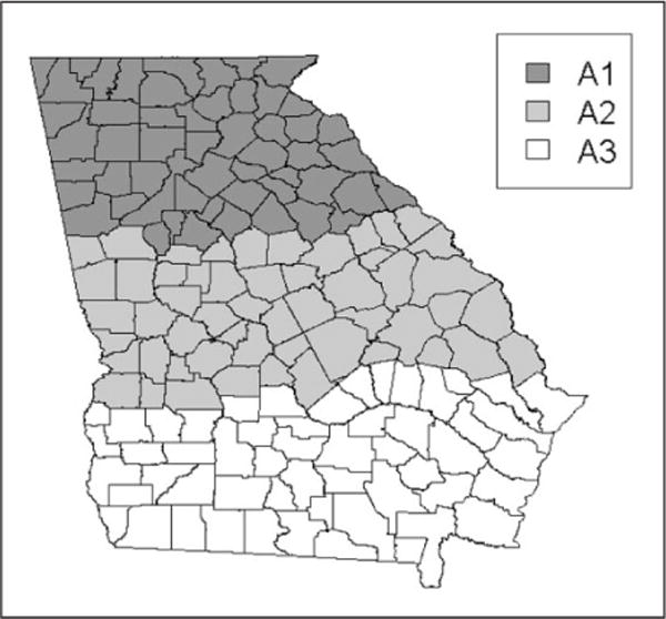
Display of the areas for the partial models.

Table 4.

Scenarios for partial models.

Notation	Meaning
PS1	S1 with ×1 and ×2 missing from A1
PS2	S2 with ×3 and ×4 missing from A2
PS3	S3 with ×1 and ×4 missing from A2 and A3
PS4	S4 with ×2 missing from A1
PS5	S5 with ×2 missing from A1
PS6	S6 with ×4 missing from A2
PS7	S7 with ×1 and ×2 missing from A1
PS8	S8 with ×2 missing from A1
PS9	S9 with ×4 missing from A2

Finally, we also explored the case that there is some unmeasured confounding in the data. This was accomplished by including a UH term and a CH term defined as u_i~Norm(0, 100) and $v_i~N\left(\frac{1}{n_i}{\displaystyle {\sum }_{i~l}{v}_l,\frac{1}{n_i{\tau }_v}}\right)$, respectively. The fixed precision values for these components are the same (1/τ_v = 0.01) so that one term does not dominate the other and lead to identifiability issues.¹⁹ Two additional simulated model scenarios result from inclusion of these random effects; the first assumes that there is simply random error present in the data, thus only the UH term is involved. This model is denoted as RE. The second model is a convolution model, denoted CV, and includes both the UH and CH terms; this model assumes that there is random error as well as error with a spatial structure. For simplicity, we only looked at this application for a subset of the simulated model scenarios (S1 for the RE model and S1, S5, S7, and S9 for the CV model).

3.2 Fitted models

In Table 5, we illustrate the three linear predictors fitted using both the model selection and BMA techniques described above. These options are appropriate for the models listed in Table 4 such that S1 up to S9 is associated with F1,…,F9. For the complete models, the suffix ‘Alt1’ represents the true model for all counties. For the partial models, the suffixes ‘Alt1’ or ‘Alt2’ represent true models for some counties depending on the descriptions in Table 4 above. ‘Alt3’ is never a true model. The different alternatives offer some models that include random noise to determine if that has an effect on which model is selected. When the RE and CV simulated models are being fitted, all linear predictor alternatives include the appropriate random effects.

Table 5.

Model alternatives.

Model	βx1	βx2	βx3	βx4	Rand. Noise
F1Alt1	Yes	Yes	Yes	Yes	No
F1Alt2	No	No	Yes	Yes	No
F1Alt3	Yes	No	No	No	No
F2Alt1	Yes	Yes	Yes	Yes	No
F2Alt2	Yes	Yes	No	No	No
F2Alt3	No	No	No	Yes	Yes
F3Alt1	Yes	No	Yes	Yes	No
F3Alt2	No	No	Yes	No	No
F3Alt3	No	No	Yes	No	Yes
F4Alt1	No	Yes	Yes	No	No
F4Alt2	No	No	Yes	No	No
F4Alt3	No	No	Yes	Yes	Yes
F5Alt1	Yes	Yes	No	No	No
F5Alt2	Yes	No	No	No	No
F5Alt3	No	Yes	Yes	No	No
F6Alt1	No	No	No	Yes	No
F6Alt2	No	No	No	No	No
F6Alt3	No	Yes	Yes	No	No
F7Alt1	Yes	Yes	Yes	Yes	No
F7Alt2	No	No	Yes	Yes	No
F7Alt3	Yes	No	No	No	No
F8Alt1	No	Yes	Yes	No	No
F8Alt2	No	No	Yes	No	No
F8Alt3	No	No	Yes	Yes	Yes
F9Alt1	No	No	No	Yes	No
F9Alt2	No	No	No	No	No
F9Alt3	No	Yes	Yes	No	No

4 Results

The results below are in relation to the implementation of the methods described above. First we present the BMS results for the complete and the partial models followed by the BMA results for the complete and partial models. Finally, we present a real data example of implementing these methods.

Note that we also collected the parameter estimates, produced for each of the alternative models, during each implementation. None of these estimates are well estimated as seen in Supplemental Table 2, but obtaining these estimates is not the goal of the model selection process. We suggest that one should refit with the selected model to obtain appropriate parameter estimates.

4.1 Complete models

All results in this section are associated with the complete models described in Table 3. The models do not allow for variation from one county to the next, and the first linear predictor alternative is the true linear predictor, thus, model weight p₁ should be the highest. Supplemental Tables 3 and 5 display the model probabilities for each scenario with BMS and BMA, respectively.

Figure 3 presents some the results for model scenarios S1–S6 fitted with corresponding models F1–F6 under the scenario of a constant expected rate (E1) and varying expected rates (E2). The figure illustrates the distribution of the model weights for the BMS procedure. These figures suggest that most models correctly select the linear predictor associated with p₁. When the evidentiary support for a particular model increases, as is the case in scenarios S7F7-S9F9, this becomes even more evident. The model selection probabilities decrease from the first to the second and third model, showing a better distinction between the models. Only in the scenarios S6F6 and S4F4, an incorrect model is selected. Note, however, that the evidence in these scenarios for the underlying model is small.

Figure 3.

Models weights associated with the complete models using BMS.

The model probabilities corresponding to scenarios E1 and E2 are similar. In most settings, it is observed that the model probability of the correct model decreases when comparing scenario E1 to E2. This indicates that model selection is more difficult when the variation in the data increases. But, differences between the model probabilities are only small, and conclusions about the selected model hardly change. The main difference we observed when comparing models in this way is that the E2 models produce lower DICs. This fact does not necessarily indicate that the E2 models fit better than the E1 models as the models have different likelihoods. These GoF measures are displayed in Supplemental Table 4.

Figure 4 displays the model probabilities associated with the complete models using the BMA technique. A completely different picture as compared to BMS is observed. These plots suggest that there is not a consistent pattern in the way that the different models perform as far as selecting linear predictors. Typically, p₁ still obtains the highest probability value, but there are several mismatches (7 of the 18 models, 38.9%). As with the BMS models, the E1 and E2 estimates continue to be nearly identical for the model probabilities while they differ when considering GoF measures. These GoF measures are displayed in Supplemental Table 6.

Figure 4.

Model probabilities associated with the complete models using BMA.

Figure 5 displays a line plot of the model probabilities for the complete models that incorporate the convolution term compared to those without the term. Through these plots, we observe a clearly selected alternative linear predictor with the BMS method for all scenarios except E1CS9F9CV. E1CS9F9CV is the scenario in which there is only a single covariate present the true linear predictor, thus it is possible that the random effects are able to explain this variation. However, the probabilities associated with p₁ in the CV models are not as large as those produced by the non-CV models. Additionally, for BMS, a majority of the model probability standard deviations are the same or smaller in value in comparison to their counterparts. Overall, BMA does not perform well in the CV model scenarios. Interestingly, for scenario E1CS1F1, BMA performs slightly better than BMS for the non-CV models in that it more clearly selects p₁ as associated with the true linear predictor, but for the CV models, BMS performs well while BMA does not. This further illustrates the detriment of BMA when extra noise is present.

Figure 5.

Model probabilities for the complete model scenarios with the CV term compared to those without the CV term.

4.2 Partial models

All results in this section are associated with the partial models described in Table 4. These models allow for variation in the linear predictors applied in different areas on the county map. Furthermore, for all models, the first or second alternatives are true for certain areas of the county map as described in Table 4, and thus model weights p₁ or p₂ should be the highest in their appropriate areas. Here, we display only a sample of the models fitted. The resulting county maps for the full range of models fit with the BMS and BMA methodology can be seen in Supplemental Figures 1 and 2, respectively.

The first set of maps shown in Figure 6 below is associated with the E1PS4F4 and E1PS8F8 scenarios using BMS. These models in particular illustrate the relationship we hope to see in the partial models. S4F4 does well to estimate p₁, but is not as accurate with p₂. In comparison, S8F8 improves the estimations of both p₁ and p₂ in that it attains higher values in the appropriate regions of the county map. In both cases, though, we continue to see a residual present in p₃. This indicates that the model can only select the correct underlying model if the parameter effect is strong enough.

Figure 6.

Model weights associated with E1PS4F4/S8F8 for BMS.

The second set of maps involving S6F6 and S9F9 displayed in Figure 7 are not as convincing, and we believe this is largely due to the fact that the true regions associated with p₁ are strictly separated to the extreme North and South of the map. There is still evidence of an improvement when moving from S6F6 to S9F9 since the regions are becoming slightly more defined as far as the maps are concerned. It may be the case that we need even more evidentiary support when the areas are separated in this manner.

Figure 7.

Model weights associated with E1PS6F6/S9F9 for BMS.

Table 6 displays the GoF measures associated with the BMS technique applied to the partial models. We continue to see smaller DIC estimates associated with the E2 models while the MSE and MSPE values are often larger. Larger MSE and MSPE estimates for E2 models are appropriate in the sense that there is more variance present in these models, thus estimation should be more difficult. Furthermore, MSE and MSPE values are nearly identical for the majority of models. In some cases, though, these estimates are quite extreme, such as for scenarios E2PS8F8 and E2PS9F9. Scenario E2PS4F4 demonstrates that outlier values in MSE are not necessarily reflected in the MSPE. Additionally, the estimates associated with A1 are typically smaller than A2 or A3. We believe this is due to the fact that this region has smaller, closer together counties. Finally, the results for the E1PS1F1RE and E1PS1F1CV models indicate that it performs very well; in fact, most of the MSE and MSPE values are smaller than those produced with E1PS1F1. This improvement continues to be the case for some of the MSE and MSPE measures related to models E1PS5F5CV, E1PS7F7CV, and E1PS9F9CV.

Table 6.

BMS GoF measures for partial models.

Model	$\overline{D}$	DIC	$\frac{\mathit{Var}\left(\overline{D}\right)}{2}$	MSEA1	MSEA2	MSEA3	MSPEA1	MSPEA2	MSPEA3
E1PS1F1	574.08	652.70	78.62	1.33	1.76	1.45	1.38	1.78	1.49
E1PS1F1RE	579.21	678.05	98.84	1.04	1.29	1.16	1.10	1.35	1.23
E1PS1F1CV	573.74	662.31	88.57	1.22	2.01	1.31	1.29	2.14	1.37
E2PS1F1	489.81	560.66	70.85	1.38	1.51	1.45	1.44	1.57	1.51
E1PS2F2	562.72	644.58	81.86	1.10	1.37	1.19	1.18	1.44	1.26
E2PS2F2	481.59	551.13	69.54	1.36	1.46	1.44	1.42	1.53	1.51
E1PS3F3	561.03	644.91	83.87	1.17	1.23	1.17	1.25	1.30	1.24
E2PS3F3	478.93	549.57	70.64	1.44	1.45	1.44	1.50	1.51	1.50
E1PS4F4	561.33	641.73	80.39	1.25	1.32	1.26	1.32	1.40	1.32
E2PS4F4	480.43	548.68	68.25	6.93	5.76	7.08	1.30	1.26	1.41
E1PS5F5	564.12	639.13	75.01	1.35	1.52	1.43	1.39	1.59	1.48
E1PS5F5CV	561.96	646.91	84.95	1.24	1.18	1.24	1.31	1.25	1.31
E2PS5F5	481.46	540.73	59.27	1.55	1.65	2.12	1.60	1.69	2.16
E1PS6F6	567.53	646.31	78.78	1.22	1.30	1.21	1.27	1.37	1.25
E2PS6F6	487.98	550.77	62.79	1.26	1.24	1.48	1.33	1.29	1.55
E1PS7F7	546.88	623.93	77.04	1.04	1.65	0.92	1.12	1.73	0.99
E1PS7F7CV	571.46	658.77	87.31	1.15	1.44	1.28	1.23	1.51	1.34
E2PS7F7	467.59	526.52	58.92	1.03	1.80	1.15	1.08	1.85	1.20
E1PS8F8	561.90	642.71	80.81	1.25	1.20	1.19	1.33	1.27	1.26
E2PS8F8	476.94	544.74	67.80	1.13	5.18	3.56	1.17	5.35	3.56
E1PS9F9	591.67	676.12	84.45	1.23	1.36	1.53	1.31	1.43	1.61
E1PS9F9CV	575.16	662.85	87.69	1.13	1.49	1.32	1.20	1.57	1.39
E2PS9F9	498.65	568.11	69.45	1.73	5.46	3.93	1.73	5.46	3.93

The sets of maps included in Figure 8 below are associated with E1PS4F4 and E1PS8F8 when fitted using the BMA technique. These maps are for comparison to the BMS fitted maps shown above in Figure 6. In comparison, we see that both fits of these models fail to be as accurate as those attained using the BMS technique. There are improvements to be noted when moving from S4 to S8 as it seems that the model probabilities are becoming slightly closer to the truth, but there is still some misrepresentation present in the estimation of p₃ since we do not expect Alt3 to be selected for any counties. Furthermore, the maps produced using the model probabilities calculated via local DIC do not produce reasonable results.

Figure 8.

Model probabilities associated with E1PS4F4/S8F8 for BMA.

As before, the next set of maps displayed in Figure 9 illustrates the fits associated with E1S6F6 and E1S9F9 when using the BMA technique. Here, we see no improvement when comparing S6 to S9, and none of the maps tend to suggest a certain region relating to one linear predictor versus another. The BMS technique continues to handle this situation better than BMA. Additionally, the DIC probability maps still fail to supply reasonable results.

Figure 9.

Model probabilities associated with E1PS6F6/S9F9 for BMA.

Figure 10 illustrates a comparison of both model selection methods’ abilities to accurately recover the truth. This comparison is accomplished by associating the probability from a specific county that should be selected to the mean probability of all counties that should not be selected for that particular model; this is described with the following formulation

$${\pi }_M=\frac{{\displaystyle {\sum }_{i=1}^{n_A}{I}_{p_{ki}\in A}\left(p_{ki}>\overline{p_{k{A}^C}}\right)}}{n_A}$$

where π_M are the probabilities displayed in Figure 10, I is an indicator function that is 1 when the enclosed logical function is true and zero otherwise, k = 1, 2 for the model probabilities p₁ and p₂, A is the area for which p_k should be highest, A^C is area A compliment, $\overline{p_{k{A}^C}}$ is the mean of the model probabilities in area A^C, and n_A is the number of counties in area A, thus i = 1, …, n_A. So, for example, with p₁ from PS1F1, a county in A2 or A3 should have a higher model probability estimate than the mean of model probabilities calculated for the counties in A1. In these plots, we see BMS performing the same or better than BMA for 21 out of the possible 36 model combinations.

Figure 10.

Model weights and probabilities associated with the misspecified models fit with E1CS1PF1.

Table 7 displays the GoF measures for the partial models using the BMA technique. The MSPE measures can be viewed in Supplemental Table 7. One of these properties is that, in general, the E2 models produce smaller DIC values but higher MSE and MSPE values for the majority of models. The difference between the MSE and MSPE values when comparing E1 and E2 for the BMA case is much larger than what we saw when using BMS. This again indicated that model selection is more difficult when there is more variation in the data. Another of these properties involves lower MSE and MSPE values for area A1; additionally, this is typically reflected in the local DIC measure for A1 as well. One new comparison that we can make with the BMA results is the local DIC measure to the BUGS calculated DIC measure, and these are different for every model. Additionally, the local DIC measure is always higher than the other DIC measure for the E1 models while this is not typically the case for the E2 models. We believe that all of these properties combined suggest that they perform better when there is no variation in the expected rates. Finally, when comparing E1PS1F1RE and the convolution models to their appropriate counterparts for the BMA models, we see that the results are still good but not better as we saw with the BMS technique, except for the local DIC measurements. The local DIC measures for these RE and CV models are much closer in value to the overall DIC measures.

Table 7.

GoF measures for BMA model fits.

	$\overline{D}$	DIC	$\frac{\mathit{Var}\left(\overline{D}\right)}{2}$	DICloc	DICA1	DICA2	DICA3	MSEA1	MSEA2	MSEA3
E1PS1F1	2455.38	2476.58	21.20	3071.80	1003.99	1045.74	1022.07	0.97	1.50	1.18
E1PS1F1RE	2240.84	2602.07	361.23	2544.09	426.93	438.86	434.01	1.10	1.71	1.34
E1PS1F1CV	2240.70	2585.74	345.03	2506.28	411.33	395.44	418.21	1.84	3.06	1.85
E2PS1F1	2097.75	2117.27	19.52	2134.62	659.53	735.26	739.83	4.84	5.01	4.46
E1PS2F2	2298.06	2487.52	189.45	2768.65	909.81	938.10	920.75	1.13	1.52	1.27
E2PS2F2	1963.62	2117.66	154.04	1882.42	587.75	630.22	664.45	5.04	4.66	3.98
E1PS3F3	2287.83	2460.36	172.52	2766.46	924.12	923.80	918.54	1.24	1.26	1.17
E2PS3F3	1954.24	2088.57	134.32	1859.04	592.31	614.52	652.21	5.62	5.59	4.24
E1PS4F3	2282.17	2451.06	168.88	2762.14	919.01	919.46	923.68	1.06	1.10	1.11
E2PS4F3	1957.81	2086.93	129.13	1871.96	592.61	622.52	656.83	4.70	3.55	4.16
E1PS5F5	2406.87	2424.65	17.78	3010.12	1009.08	995.17	1005.88	1.06	1.18	1.14
E1PS5F5CV	2215.47	2532.20	316.73	2532.87	399.21	497.95	390.56	2.03	1.70	2.44
E2PS5F5	2051.09	2067.67	16.59	2045.27	660.59	676.37	708.31	4.96	4.01	5.49
E1PS6F6	2394.56	2402.73	8.17	2976.58	990.09	985.44	1001.04	0.96	0.93	0.98
E2PS6F6	2049.45	2057.78	8.33	2048.56	646.80	681.73	720.04	4.84	3.53	4.39
E1PS7F7	2445.02	2481.95	35.93	3135.98	1000.75	1157.03	978.19	1.05	2.59	1.23
E1PS7F7CV	2256.02	2578.49	322.47	2576.23	400.95	397.55	500.68	1.80	3.07	1.82
E2PS7F7	2093.38	2125.59	32.21	2250.22	656.83	816.61	776.79	3.68	7.89	3.98
E1PS8F8	2291.10	2465.30	174.20	2773.70	924.77	919.42	929.51	1.46	1.39	1.43
E2PS8F8	1949.31	2079.34	133.03	1859.86	601.57	597.40	660.88	4.32	4.61	5.25
E1PS9F9	2513.67	2525.15	11.48	3137.71	1043.27	1005.20	1089.23	1.08	2.88	1.46
E1PS9F9CV	2268.81	2604.85	336.05	2582.19	403.25	505.59	392.36	1.88	3.09	1.93
E2PS9F9	2126.08	2137.42	11.34	2150.69	692.09	689.33	769.27	4.11	4.58	6.30

4.3 Misspecified models

In our research, we also misspecified models such that we fit the complete simulated data sets with the partial method and vice versa. In particular, we did this with models E1CS1 and E1PS1 because they performed well initially in both the BMS and BMA methodology. These appropriately specified results can be seen in Supplemental Tables 3 and 5 above for the complete models as well as Supplemental Figures 1 and 2 for partial models.

The results from fitting partial simulated data (E1PS1) using the appropriate complete model (CF1) are in Table 8. They show the BMS method choosing the linear predictor associated with p₁ while BMA selected the linear predictor associated with p₃. The true linear predictors here could be p₁ or p₂ depending on the county. We suspect that the BMA method incorrectly selects p₃ because the first two linear predictors are alternating as the true model for the different counties. For example, if p₃ = 0.4 for all counties while p₁ and p₂ alternate between the values 0.1 and 0.5 depending on the county of interest, we could get similar results. The GoF measures are quite different for these two methods, but this is similar to the previous results in Section 4.1.

Table 8.

Model weights, probabilities, and GoF measures for the misspecified models.

	p1	p2	p3	$\overline{D}$	DIC	$\frac{\mathit{Var}\left(\overline{D}\right)}{2}$
E1PS1CF1 BMS	0.551	0.333	0.470	609.15	614.43	5.27
E1PS1CF1 BMA	0.283	0.283	0.419	2315.38	2483.11	167.73
E1CS1PF1 BMS	0.498a	0.500a	0.497a	575.54	674.23	98.69
E1CS1PF1 BMA	0.256a	0.248a	0.253a	2437.01	2459.70	22.70

^aThese values are means of the weights and probabilities that are actually varying across counties.

When fitting the complete simulated data (E1CS1) to the appropriate partial fitted model (PF1), we expect to see the linear predictor associated with p₁ selected for all counties, and the county maps for this misspecification are displayed in Figure 11. Both methods’ results still show some variability among the different counties, but the BMA method clearly selects the linear predictor associated with p₂ for the northern counties. The GoF measures as well as mean probabilities and weights are shown in Table 8.

Figure 11.

County weights based on the BMS and BMA procedures for the misspecified models.

4.4 Colon cancer data example

For our real data example, we use 2003 colon cancer data in the state of Georgia as an outcome and predictors from the Area Health Resources Files (AHRF) dataset²⁰ (median household income (in thousands of dollars), percent persons below poverty level (PPBPL), unemployment rate of those aged 16 or greater, and percent African American population). Past studies suggest that colon cancer has a spatial structure and is related to these predictors, though they are not the main risk factors associated with colon cancer.^21–24 Our three possible linear predictors all contain an uncorrelated random effect, and they differ by the predictors included. The first linear predictor includes all of the covariates while the second includes only income and percent African American population. The third linear predictor includes PPBPL and percent African American population. We alternate income and PPBPL in the second two linear predictors because they are correlated (ρ = −0.897). Also note that we standardized the continuous covariates before fitting the models because this was necessary for the BMA fitting.

The results from fitting these models with the real data using the BMS method are displayed in Figure 12 and suggest that it may be beneficial to use the second linear predictor option in the northern and western areas of the state while the third linear predictor option may be optimal for the southern and western counties. From these results, we can also see that it is beneficial to place correlated covariates in separate linear predictors and allow the BMS process to determine which is appropriate for the different counties.

Figure 12.

County weights based on the BMS procedure for the colon cancer example.

The BMA method produces two options for p-values, and we note different results between those two options as well as the results produced for the model selection method. The BMA model probability results shown in Figure 13 suggest that the first linear predictor option should be used for the Northern counties while the second linear predictor option seems appropriate for the Southern counties. The results also suggest that the third linear predictor may also be useful for the mid-Eastern counties. The DIC calculated probabilities do not show a favorable pattern for any of the linear predictor options; these probabilities produce very random plots much alike those seen in Supplemental Figure 2.

Figure 13.

County weights based on the BMS procedure for the colon cancer example.

The model re-fits using the results above and applying them to the selected areas of the map suggest that qualitatively using the two model selection methods in combination produce the best results. We found the most convincing results in the data when the second linear predictor was applied to the Northern counties of the state (area A1 described previously) while the third linear predictor was most appropriate for the Southern counties of the state (areas A2 and A3). These re-fits were better than simply using the set of selected counties from either model selection technique on its own, but we believe this is largely because the number of counties selected was somewhat small. Supplemental Table 8 displays parameter estimates associated with fitting the second and third linear predictors to the full county map as well as the selected regions.

5 Discussion

Based on the simulation results and from a qualitative assessment, we believe that the BMS technique outperforms BMA in terms of selecting the appropriate linear predictors. The results for the BMS method are also more consistent when comparing different scenarios such as E1 versus E2, and S1F1-S9F9 to their appropriate counterparts. Furthermore, we discovered that the BMS technique is more robust to misspecified models. For both techniques, the complete models tend to recover the truth more efficiently and accurately than the partial models, but this is to be expected as these models are not as complex.

We also see significant improvements in recovering the appropriate estimates when comparing the models whose data sets have true parameter estimates with larger magnitudes, meaning there is more evidentiary support in the data. This is evident in complete, partial, E1, and E2 models as well as both BMS and BMA techniques. As far as GoF measures are concerned, DICs cannot be compared across models due to different outcome variables, and thus different likelihoods. The MSE and MSPE estimates suggest that, for the most part, the E1 models fit better than the E2 models. We also note that the A1 region often offers the lowest MSE and MSPE measures. We believe that this occurs because the counties in the A1 region are smaller and closer together than the others. Additionally, more often than not, S7F7-S9F9 models produce lower MSE and MSPE values. This suggests that the techniques perform better when there is more support in the data.

There are several obstacles that can be encountered when performing both model selection methods. The first of these involves the strength of association present in the data. If there is not enough evidence in the data, we have seen that both BMS and BMA fail to perform well.

Another issue involves extra noise in the data. As in many statistical applications, extra variation in the data can lead to difficulties in estimation; BMS and BMA are not immune to this issue. By the same token, including an uncorrelated random effect in one of the alternative linear predictors when it is not truly needed can also result in an improper selection of a linear predictor. In many cases, though, there is random noise present in data, and including that random effect can be helpful. This is why random effects were included in all linear predictor alternatives for our real data example. Furthermore, we did include several scenarios in our simulation study (RE and CV models) that introduce this extra noise and fit the models such that the noise is also reflected in the true and alternative linear predictors. In this situation, the results suggest that both methods seem to perform comparably when uncorrelated extra variation was imposed upon the data. When the convolution term was present in the model, BMS continued to perform well most of the time while BMA suffered in its ability to recover the truth. Here, the BMS method produced slightly smaller MSE and MSPE values than those produced with model scenarios that exclude these random terms.

One shortcoming of both of these methods is that they must be performed in sequence with an additional model fit to determine the parameter estimates associated with the selected linear predictor or predictors in the case that one predictor is more appropriate in a certain region of the state. This is a shortcoming that adds to the complexity of the model fitting process, but it is worth pursuing to obtain the most appropriate results.

6 Conclusion

From this comparison between our proposed BMS and BMA, we conclude that the BMS application qualitatively produces more accurate as well as more precise results than those produced by BMA in terms of selecting the appropriate linear predictors across maps. There still may be some instances, though, where BMA is the preferred method because one is able to calculate the local DICs in that situation.

References

- 1.Clyde M, Iversen ES. Bayesian model averaging in the M-open framework. In: Damien P, Dellaportas P, Polson NG, Stephens DA, editors. Bayesian theory and applications. Oxford: Oxford University Press; 2015. [Google Scholar]
- 2.Hoeting JA, Madigan D, Raftery AE, et al. Bayesian model averaging: a tutorial. Stat Sci. 1999;14:382–417. [Google Scholar]
- 3.Lesaffre E, Lawson AB. Bayesian biostatistics. 1. West Sussex, UK: Wiley; 2013. p. 534. [Google Scholar]
- 4.Lunn D, Jackson C, Best N, et al. The BUGS book: a practical introduction to bayesian analysis. 1. Boca Raton, FL: CRC Press; 2013. p. 399. [Google Scholar]
- 5.Thomas A, O’hara B, Ligges U, et al. Making BUGS open. R News. 2006;6:12–17. [Google Scholar]
- 6.George EI, Clyde M. Model uncertainty. Stat Sci. 2004;19:81–94. [Google Scholar]
- 7.Bondell HD, Krishna A, Ghosh SK. Joint variable selection for fixed and random effects in linear mixed-effects models. Biometrics. 2010;66:1069–1077. doi: 10.1111/j.1541-0420.2010.01391.x. [DOI] [PMC free article] [PubMed] [Google Scholar]
- 8.Garcia RI, Ibrahim JG, Zhu H. Variable selection for regression models with missing data. Statistica Sinica. 2010;20:149–165. [PMC free article] [PubMed] [Google Scholar]
- 9.Hoeting JA, Raftery AE, Madigan D. Bayesian variable and transformation selection in linear regression. J Comput Graph Stat. 2002;11:485–507. [Google Scholar]
- 10.Rockova V, George EI. Negotiating multicollinearity with spike-and-slab priors. Metron. 2014;72:217–229. doi: 10.1007/s40300-014-0047-y. [DOI] [PMC free article] [PubMed] [Google Scholar]
- 11.Scheel I, Ferkingstad E, Frigessi A, et al. A Bayesian hierarchical model with spatial variable selection: the effect of weather on insurance claims. J Royal Stat Soc Ser C, Appl Stat. 2013;62:85–100. doi: 10.1111/j.1467-9876.2012.01039.x. [DOI] [PMC free article] [PubMed] [Google Scholar]
- 12.Hans C. Model uncertainty and variable selection in Bayesian lasso regression. Stat Comput. 2009;20:221–229. [Google Scholar]
- 13.Li J, Das K, Fu G, et al. The Bayesian lasso for genome-wide association studies. Bioinformatics. 2011;27:516–523. doi: 10.1093/bioinformatics/btq688. [DOI] [PMC free article] [PubMed] [Google Scholar]
- 14.Viallefont V, Raftery AE, Richardson S. Variable selection and Bayesian model averaging in case-control studies. Stat Med. 2001;20:3215–3230. doi: 10.1002/sim.976. [DOI] [PubMed] [Google Scholar]
- 15.Lawson AB. Bayesian disease mapping: hierarchical modeling in spatial epidemiology. 2nd. Boca Raton, FL: CRC Press; 2013. [Google Scholar]
- 16.Wheeler DC, Hickson DA, Waller LA. Assessing local model adequacy in Bayesian hierarchical models using the partitioned deviance information criterion. Computat Stat Data Analys. 2010;54:1657–1671. doi: 10.1016/j.csda.2010.01.025. [DOI] [PMC free article] [PubMed] [Google Scholar]
- 17.Schlather M. Introduction to positive definite functions and to unconditional simulation of random fields. Lancaster: Lancaster University; 1999. [Google Scholar]
- 18.Diggle PJ, Ribeiro PJ., Jr . Model-based geostatistics. 1. New York: Springer-Vertag; 2007. p. 232. [Google Scholar]
- 19.Eberly LE, Carlin BP. Identifiability and convergence issues for Markov chain Monte Carlo fitting of spatial models. Stat Med. 2000;19:2279–2294. doi: 10.1002/1097-0258(20000915/30)19:17/18<2279::aid-sim569>3.0.co;2-r. [DOI] [PubMed] [Google Scholar]
- 20.Area Health Resource Files (AHRF) Rockville, MD: US Department of Health and Human Services, Health Resources and Services Administration, Bureau of Health Workforce; 2003. [Google Scholar]
- 21.American Cancer Society. Colorectal cancer facts & figures. Atlanta, GA: American Cancer Society; [Google Scholar]
- 22.DeChello LM, Sheehan TJ. Spatial analysis of colorectal cancer incidence and proportion of late-stage in Massachusetts residents: 1995–1998. Int J Health Geograph. 2007;6:20. doi: 10.1186/1476-072X-6-20. [DOI] [PMC free article] [PubMed] [Google Scholar]
- 23.Elferink MA, Pukkala E, Klaase JM, et al. Spatial variation in stage distribution in colorectal cancer in the Netherlands. Eur J Cancer. 2012;48:1119–1125. doi: 10.1016/j.ejca.2011.06.058. [DOI] [PubMed] [Google Scholar]
- 24.Henry KA, Sherman RL, McDonald K, et al. Associations of census-tract poverty with subsite-specific colorectal cancer incidence rates and stage of disease at diagnosis in the United States. J Cancer Epidemiol. 2014;2014:823484. doi: 10.1155/2014/823484. [DOI] [PMC free article] [PubMed] [Google Scholar]
Associated Data
This section collects any data citations, data availability statements, or supplementary materials included in this article.