Nonparametric Estimates of Gene × Environment Interaction Using Local Structural Equation Modeling

Abstract

Gene × Environment (G×E) interaction studies test the hypothesis that the strength of genetic influence varies across environmental contexts. Existing latent variable methods for estimating G×E interactions in twin and family data specify parametric (typically linear) functions for the interaction effect. An improper functional form may obscure the underlying shape of the interaction effect and may lead to failures to detect a significant interaction. In this article, we introduce a novel approach to the behavior genetic toolkit, local structural equation modeling (LOSEM). LOSEM is a highly flexible nonparametric approach for estimating latent interaction effects across the range of a measured moderator. This approach opens up the ability to detect and visualize new forms of G×E interaction. We illustrate the approach by using LOSEM to estimate gene × socioeconomic status (SES) interactions for six cognitive phenotypes. Rather than continuously and monotonically varying effects as has been assumed in conventional parametric approaches, LOSEM indicated substantial nonlinear shifts in genetic variance for several phenotypes. The operating characteristics of LOSEM were interrogated through simulation studies where the functional form of the interaction effect was known. LOSEM provides a conservative estimate of G×E interaction with sufficient power to detect statistically significant G×E signal with moderate sample size. We offer recommendations for the application of LOSEM and provide scripts for implementing these biometric models in Mplus and in OpenMx under R.

Gene × Environment (G×E) interaction studies test the hypothesis that the strength of genetic influence varies across environmental contexts, or equivalently, that environmental effects vary as a function of genotype (Plomin et al., 1977). Twin and family behavior genetic studies test for G×E by estimating latent biometric variance components, typically additive genetic effects (A), shared environmental effects (C), and nonshared environmental effects (E), and examining whether the magnitudes of these variance components differ at different levels of a measured environmental variable.¹ When the measured environment is composed of a small set of discrete categories, testing for G×E is straightforward; however, in many cases the measured environment is a continuous variable. Existing methods for estimating G×E with continuously measured environmental variables require a priori specification of the interaction’s functional form (Purcell, 2002). If the wrong function has been specified, inferences may be biased and, at times, G×E effects present in the data may not be detected.

In the current paper, we present a nonparametric method for estimating the shape of G×E interaction in twin and family data and provide scripts for implementing this technique in Mplus (Muthén & Muthén, 1998–2010) and OpenMx (Boker et al., 2011). This method can help researchers better understand patterns in their data and can improve model selection and testing in the analysis of G×E interaction. In the following sections, we first present extant approaches to estimating G×E interaction in biometric twin and family models when the environmental moderator is measured at the family-level (i.e., is shared by members of the twin pair). We then present the novel approach, illustrate it with a real data analysis application followed by several simulation studies, and finally discuss its strengths and limitations.

Existing Models for G×E

Categorical G×E Model

When the environmental moderator is categorical (e.g. impoverished vs. not impoverished), estimating G×E is a straightforward application of multiple-group structural equation modeling (Neale & Maes, 2005, Chapter 9). In the case of a dichotomous moderator and an ACE model fit to data from monozygotic twins reared together (MZ) and dizygotic twins reared together (DZ), instead of the usual two-group model (one group for MZ twins and a second for DZ twins), a four-group model is fit (with additional groups for “low risk” and “high risk” environments each for MZ and DZ twins). Such a model is represented in Figure 1A. Each of the A, C, and E component paths has two labels (e.g. a_l and a_h) to indicate that the parameter is estimated separately for the low (“l”) and high (“h”) risk levels of the moderator. To test for G×E, parameters for the low and high risk models are constrained to be equal and compared by a χ² test to one in which they are allowed to differ between the environmental exposure groups. If the “a” (or c or e) parameters cannot be constrained to be equal across environmental exposure groups without significant loss of model fit, then the G×E hypothesis is supported, as the genetic or environmental variance estimate (e.g., a²) significantly differs across groups.

Figure 1.

Path diagrams representing each type of G×E model. In all models, latent additive genetic (A), shared environmental (C), and nonshared environmental (E) factors with are estimated for a phenotype for twin1 (Y1) and a phenotype for twin2 (Y2). The A factors correlate at 1.0 for monozygotic twins and at 0.5 for dizygotic twins. The C factors correlate at 1.0, and the E factors are uncorrelated. A. Categorical G×E in which separate parameters are estimated for low risk (a_l, c_l, e_l, and μ_l) and high risk (a_h, c_h, e_h, and μ_h) environments. B. Parametric G×E model in which the focal pathways are specified to be a linear combination of parameters representing main effects (a, c, e) and interaction terms (a′, c′, and e′) of the ACE components with the moderator (M). The main effect of M is represented as a “moderated mean” (b₁). The intercept of the phenotype is also estimated (b₀). C. Nonparametric LOSEM G×E model in which local parameters for each level of the moderator are estimated (â_M, ĉ_M, ê_M, ${\widehat{\mathrm{\mu }}}_{\mathrm{M}}$), noting the circumflex refers to the fact that these parameters are based on weighted data rather than data precisely at the level of M. The subscript [−m…0…+m] refers to the fact that the parameters are actually vectors that include weighted estimates from a lower bound of M to an upper bound of M.

In cases in which the environmental moderator has been measured continuously, a researcher could categorize the environmental moderator variable by collapsing ranges of the environment into discrete bins. If there is reason to be specifically interested in discrete levels of environmental exposure, or if a researcher has a strong a priori reason to expect a discontinuous G×E effect at a known cut point, this categorical approach may be optimal. Without strong guidance from theory or past research, however, researchers must make arbitrary or intuitive decisions regarding the number of bins to use and the ranges of the environment to cluster (i.e., the location of the cut points). Important aspects of the interaction may be obscured if large bins are selected, or results may be excessively noisy if small bins are selected. Such decisions offer experimenter degrees of freedom (Simmons et al., 2011) and may possibly lead to false discovery (Benjamini & Hochberg, 1995).

Parametric G×E Model

Purcell (2002) introduced an extension of the classical twin model for the analysis of G×E interaction with continuously measured environmental moderators. As depicted in Figure 1B, this parametric G×E model controls for the main effect of the observed moderator on the phenotype. Moreover, it specifies that the regression paths from latent biometric factors (A, C, and E) to the phenotype are parametric functions of the observed moderator. When the regression paths are specified to be linear functions of the moderator (as is depicted in Figure 1B), ACE variance component estimates are quadratic functions of the moderator (as the regression path must be squared in order to produce a variance expectation). When the biometric interaction model is expanded to include both linear and quadratic interactions on the paths (such that the ACE variance estimates are quartic with respect to the moderator), one can test whether genetic variance is an inverted U-shaped curve, with the highest genetic variance in the “average” environment (e.g., Burt et al., 2006). Others (e.g. Turkheimer & Horn, 2014) have endorsed exponential functions.² Still others have considered how to test for G×E when the moderator is not necessarily shared by members of a twin pair, but may differ between twins, thus allowing for the simultaneous consideration of gene-environment correlation (e.g., Johnson, 2007; Medland et al., 2009; Molenaar & Dolan, 2014; Price & Jaffee, 2008; Rathouz et al., 2008; Schwabe & van den Berg, 2014; van der Sluis et al., 2012; van Hulle et al., 2013). We do not recapitulate these theoretical and technical issues here, but simply refer the reader to this previous literature, and note here that these multivariate extensions also model the paths from the biometric components to the phenotypes as parametric functions of the moderator.

LOSEM: LOESS with Latent Variables

As noted above, categorical G×E is of limited utility when an environmental moderator of interest is truly continuous (e.g., socioeconomic status), because this approach lumps together potentially distinct environmental contexts, risks cutting the data at suboptimal points, or loses information concerning the environmental variable. Parametric G×E solves these problems by retaining the full continuous range of the environmental variable. Yet parametric G×E models can still be limiting because the functional form (or competing functional forms) of the interaction must be chosen a priori. Researchers may not have strong theoretical predictions regarding how potential moderating effects play out in particular parts of the environmental range, or they may suspect that the polynomial function they are estimating is not capturing theoretically relevant effects. Creating a flexible, yet powerful and informative, tool to investigate varying levels of genetic influence on phenotypes is a critical goal for behavior genetic methodology (e.g., Kirkpatrick, McGue, & Iacono, 2015; Logan et al., 2012; Zheng & Rathouz, 2015).

Local structural equation modeling (LOSEM) is a method developed by Hildebrandt et al. (2009, see also Hülür et al., 2011; Schroeders et al., 2015) to generate nonparametric estimates of differences in structural equation model parameters across different levels of a measured putative moderator. LOSEM is the latent variable analogue of LOESS (LOcal regrESSion), or locally weighted regression (Cleveland & Devlin, 1988), a nonparametric regression method that fits a “smoothed” line (a loess curve) through the cloud of data points. Both methods draw on kernel regression techniques, in which statistical models are locally estimated for kernels of the data (Li & Racine, 2007). In this context, the term kernel refers to a weighting function used to select datapoints to be used in local analyses. A variety of nonparametric regression techniques are common in many areas of scientific investigation and have proven highly valuable to for gaining insight into the nuances of empirical phenomena (e.g., Eubank, 1999; Fox, 2000; Green & Silverman, 1994; Hart, 1997; Horowitz, 2009; Takezawa, 2012). Key strengths of nonparametric approaches include consistent estimation (i.e., no matter the underlying functional form, nonparametric estimation will converge on the true form given large enough sample size, which is not the case for mis-specified parametric estimation) and primary reliance on data visualization (i.e., flexible trend lines), rather than dichotomous significance levels or static estimates, to better understand empirical relations. Such approaches have been widely used in standard regression contexts, but have only recently been adapted for structural equation modeling.

In the following sections, we explain how LOSEM can be applied to produce a nonparametric “smoothed” estimate of how genetic and environmental variances differ across the observed range of a measured family-level environment. Overall, LOSEM involves running a large number of models, one for each “target” value of the moderator, and the estimates from all models are combined into a nonparametric representation of how parameters differ across the range of the moderator. The use of the LOSEM approach has the potential to illuminate patterns of G×E that may otherwise be obscured, and may help guide researchers toward selecting the most appropriate parametric G×E models.

Step 1: Specify a general model

First, a general biometric structural equation model is specified exactly as would be done in a non-G×E context. Note that although the hypothesis being examined predicts that some of the parameters of this model differ as a function of a moderator variable, this moderator is not included in the general structural equation model. In the simplest case, in which one is interested in whether the paths from the biometric components to a phenotype differ as a function of the moderator, the specified model would simply be a classical univariate twin ACE model. (Of course, alternate univariate forms are possible, such as a dominant genetic model, or a model without a shared environmental estimate.) Because the nonparametric approach does not require any moderation effects to be specified explicitly in the general model, it is also easily applied to more complex multivariate models (e.g., Cholesky decomposition, correlated factors model, simplex, etc.; Neale & Maes, 2005) or to alternative parameterizations (e.g., Molenaar & Dolan, 2014; Schwabe & van den Berg, 2014). The primary parameters of interest are the pathways from the latent genetic and environmental factors to the phenotype, which, when squared, represent the variance accounted for by the ACE components.

Step 2: Select a range of target values of the moderator

Second, a moderator and range of target values of the moderator are selected. For instance, one might be interested in estimating latent genetic and environmental influences on a phenotype across the socioeconomic status (SES) range from 2 SD below the mean SES to 2 SD above the mean SES. (Care should be taken to avoid extremely high and low value of the moderator, e.g., +/- 3 SD, as the effective sample size may become small and the estimates imprecise.) If SES is on a z-scale, the target values of the moderator would be a vector from −2 to +2. To gain sufficient clarity of the trends, the vector could include increments of .1 or even .01. Importantly, this decision is not the same as the decision regarding how many bins to use in a categorical G×E model. The LOSEM approach uses the entire dataset for every model, whereas binning separates data into discrete subsets. By using smaller intervals for the target value of the moderator in the LOSEM approach, one simply reduces the distance between estimates (i.e. the resolution of the trend), but the estimates do not change depending on the interval. Choosing smaller interval sizes also does not reduce the effective sample size, because the weighting function does not depend on the interval size (see below for further discussion of the weight function). The only tradeoff for choosing very small intervals is computation time.

Step 3: Specify a weight function

Third, a weight function is specified, so that observations (i.e., rows of data in the model) are weighted by their distance from a target value of the moderator. For instance, individuals for whom the moderator = 1 will be weighted most highly when the target value is 1, but weighted much less when the target value is −1. In this way, every row in the dataset is informative at all levels of the target, but observations that are closest to the location of the target value of the moderator are privileged (weighted more highly) compared to distant observations.

We follow Hildebrandt et al. (2009) and Gasser et al. (2004) in recommending that weights be calculated based a kernel function in which the bandwidth (bw) depends on the total sample size (N pairs of twins) and the variability of the moderator (SD_M):

$$\mathit{bw}=2\ast N{(}^{-1/5})\ast {\mathit{SD}}_{\mathrm{M}}$$

This bandwidth selection is designed to minimize and balance the amount of bias (i.e., oversmoothing) and variability (i.e., undersmoothing) in the produced estimates (Hart, 1997, p. 12; Li & Racine, 2007). As the bandwidth is progressively expanded, the weighting function approximates a uniform distribution across the moderator, and the “local” results actually weight all of the data equally. In this case, the estimates will not capture any moderation trends. As the bandwidth is progressively shrunk, the weighting function privileges only data at or near a specific level of the moderator. We return to alternative specifications of the weighting function in the discussion.

The distance (z_i) between the value of M for each individual i and the target value of M is then scaled according to bw:

$${\mathrm{z}}_{\mathrm{i}}=(M_{\mathrm{i}}-\text{target}M)/\text{bw}$$

The kernel weights (K)³ for each individual i, for each target value of M, are then calculated based on this distance, and re-scaled as final weights (W) that vary between 0 and 1:

$$\begin{array}{c}\mathrm{K}=(1/\surd 2\mathrm{\pi })\ast \text{exp}({-{\mathrm{z}}_{\mathrm{i}}}^2/2)\\ \mathrm{W}=\mathrm{K}/.399\end{array}$$

Figure 2 shows example weighting distributions. The distribution of weights varies as a function of sample size and the standard deviation of the moderator. Larger sample sizes and smaller standard deviations of the moderator both result in weighting distributions more tightly focused around the target moderator value. Figure 2A illustrates weighting distributions based on data used in the current study (N = 650, moderator SD = 1).⁴ Figure 2B shares the moderator SD of Figure 2B, but is based on a ten times larger sample (N = 6500) to demonstrate how the distribution of weights shrinks with larger samples. The bw parameter is the primary determinant of the width of the weighting distribution. Researchers may easily manipulate this parameter to produce different levels of smoothing.

Figure 2.

Example distributions of weighting variable (y-axis) at three target levels of the moderator (x-axis). Data closer to the target level of the moderator carries more weight in the analysis. The distribution around the target is smaller with larger sample size and smaller standard deviation of the moderator. A. Distribution for the current analysis based on data from ECLS-B (N = 650, SD = 1). B. Distribution for hypothetical analysis based on data from ECLS-B with ten times the number of participants.

Step 4: Run the model for each target value of the moderator and compile estimates

Finally, the biometric model of interest is estimated once at each target value of the moderator, each time weighting the observations by their distance from the current target.⁵ Thus, if one were interested in characterizing genetic and environmental influences across −2 SD SES to +2 SD SES in increments of .01, a total of 401 ACE models would be estimated. Each model would be based on the full dataset, but would give different weight to the data based on the specified target level of the moderator. To examine the obtained nonparametric G×E curve, the user may then plot parameters of interest (e.g., the squared additive genetic path from the A factor to phenotype) as a function of the value of the target moderator. This approach renders the nonparametric function of the genetic variance moving smoothly across values of the environmental moderator.

The LOSEM approach to G×E is shown as a path diagram in Figure 1C. Each parameter is estimated at each of a range of target values of the continuous moderator (in Figure 1C we specify this range in terms of “m” units above and below a mean of 0), and this information is aggregated to yield a nonparametric function of the parameter estimates across the chosen range of the moderator. To summarize, LOSEM involves running a large number of models, one for each “target” value of the moderator, and the estimates from all models are combined into a nonparametric representation of how parameters differ across the range of the moderator.

Work flow and implementation in Mplus and R

The online supplement includes example scripts to implement LOSEM. For analysts using Mplus (Muthén & Muthén, 1998–2010), automating the multiple models that need to be run can be accomplished using the “MplusAutomation” package in R (Hallquist, 2011; R Development Core Team, 2013). This package includes commands to (1) create multiple modified input files based on a template, (2) run all of the input models, and (3) extract and combine model parameters from the output files (see Appendix A–C for sample scripts). R can then be used to extract model parameters and bind these into a dataset across target levels of the moderator with associated model parameters and standard errors. This dataset can then easily be used to plot nonparametric G×E interaction trends. Using OpenMx (Boker et al., 2011), the functionality of R can be used to accomplish similar tasks directly (see Appendix D for sample scripts). These packages make it extremely easy to run, extract, and aggregate all of the necessary models and parameter estimates. The whole process can take as little as 15 minutes.

In the sections that follow, we demonstrate the power of this approach by re-analyzing gene × SES findings and show a potentially novel pattern of result that would have been obscured had LOSEM not been employed. We test the operating characteristics of LOSEM by simulating datasets where the functional form of the G×E effect is known and compare LOSEM results with results from standard parametric models. Finally, we make several methodological recommendations concerning the judicious application of LOSEM.

Study 1: Childhood SES and Genetic Effects on Cognitive Ability in ECLS-B

We have previously used LOSEM in a study of how birth cohorts differ in genetic influences on fertility behavior (Briley et al., 2015) and in a study of how the relation between pubertal timing and depression varies as a function of SES (Mendle et al., 2015). In both of these cases, we expected nonlinear G×E trends, but it was unclear what the exact functional form was. LOSEM allowed us to explore the data and make informed analytic choices. Here we present another example of LOSEM for the analysis of G×E interaction using data from the Early Childhood Longitudinal Study – Birth Cohort (ECLS-B; Snow et al., 2009). Previous publications have reported results of parametric gene × SES interaction analyses in this dataset. Tucker-Drob et al. (2011) reported that longitudinal increases in mental ability between 10 months and 2 years were more heritable among children being raised in higher SES families. Rhemtulla and Tucker-Drob (2012; also see Tucker-Drob & Harden, 2012) reported that age 4 math, but not age 4 reading, was more heritable among children being raised in higher SES families.

These results are consistent with a bioecological model, in which resource-rich environments allow for personal interests, preferences, desires, and temperaments to play a large role in development (e.g., Bronfenbrenner & Ceci, 1994; Tucker-Drob et al., 2013). However, alternative theoretical models have been proposed, in which there is a nonlinear relation between environmental circumstances and the genetic variance of cognition (e.g., Scarr, 1992; Turkheimer & Gottesman, 1991). Under a model of the “average expectable environment” (Scarr, 1992, p. 5), genetic variance is predicted to increase as the environment transitions from poor to average, but then plateau following. According to this perspective, there is a dramatic difference between growing up in poverty and growing up in the middle class, but a less appreciable difference between growing up middle class and wealthy.

By applying LOSEM to model the shape of the G×SES interactions, we seek to determine whether SES-related increases in genetic variance occur throughout the range of the SES distribution or are confined to a specific range of the SES distribution. We apply LOSEM to all six cognitive phenotypes available in ECLS-B: 10 months Bayley mental development, age 2 years Bayley mental development, age 4 years math and reading readiness, and kindergarten math and reading achievement. For methodological details on the ECLS-B sample and measurement of these phenotypes, including sample statistics, please see Rhemtulla and Tucker-Drob (2012), Tucker-Drob and Harden (2012), Tucker-Drob (2012), and Tucker-Drob et al. (2011).

Results

Figure 3 compares LOSEM results with traditional parametric results (Purcell, 2002). The first two columns present variance in the phenotype accounted for by ACE factors. Dotted lines represent +/- 1 standard error of the estimate. The last two columns present the main effect of the moderator. For the LOSEM approach, the graph plots the estimated mean of the phenotype (i.e., the estimated twin mean of cognitive ability at SES = −2 to +2). For the parametric approach, the graph plots the regression parameter for the main effect of SES. Table S1 and Supplementary Files S1–2 present parameter estimates and model fit statistics for models fit for the current study and a more complete analytic description. In the context of the parametric model, we found significant genetic interaction terms for age 2 Bayley (a′ = .193, p < .001) and age 4 math (a′ = .164, p < .001). Significant interaction terms for the shared environment (c′ = .106, p < .01) and the nonshared environment (e′ = .075, p < .001) were found for age 4 reading. No other interaction terms were significant for the standard application of the parametric model. Higher levels of SES were associated with higher levels of ability; these regression coefficients ranged from .030 (n.s.) to .476 (p < .001, see Table S1).

Figure 3.

Comparison of LOSEM and parametric gene × socioeconomic status results for cognitive ability measures from ECLS-B. A. Age 10 months Bayley. B. Age 2 years Bayley. C. Age 4 years Math Achievement. D. Age 4 years Reading Achievement. E. Kindergarten Math Achievement. F. Kindergarten Reading Achievement.

Across most models, there was generally good consilience between the LOSEM results and the parametric specification. The approaches largely agree on the directional trend of the variance components. For age 1 and age 2 Bayley, shared environmental influences decrease, nonshared environmental influences decrease slightly, and genetic influences increase with increasing SES across both analytic approaches. The general directional trends are also very similar for age 4 math and reading. The results are less consistent for kindergarten math and reading. The LOSEM results imply fluctuating levels of genetic and environmental influences, but the parametric results imply very little change in parameters across different SES levels.

Despite the general agreement between approaches in broad trends, a few substantial differences are evident. Most notably, the linear parametric interaction model for kindergarten reading ability (Figure 3F) is clearly mis-specified. The LOSEM results indicate relatively low genetic variance at low SES, a spike in genetic variance near average levels of SES, and a steep decline in genetic variance at high levels of SES. The linear specification of the parametric model indicates that there is essentially no difference in genetic variance across SES, obscuring rather large differences apparent in the LOSEM results. Figure 4 presents a specification of the parametric model that includes a quadratic interaction term, which is significant for genetic influences (see Table S1).

Figure 4.

LOSEM, linear parametric, and nonlinear parametric model for Kindergarten reading achievement.

As discussed earlier, alternate theories of child development make competing predictions regarding where in the research range of interest of the moderator most of the increases or decreases in genetic variance occur. In particular, the “average expectable environment” model predicts the largest difference to be between poor and good-enough environments, not between good and excellent environments. The LOSEM approach easily captures this important information. On the other hand, the parametric model, due to its specification, tends to predict more extreme increases for more extreme values of the moderator. At least for the six phenotypes under investigation in the current study, this does not seem well-warranted.

Table 1 compares differences in the magnitude of genetic variance across meaningful levels of the moderator for each analytic approach. In particular, we were interested in whether interaction effects were concentrated at the low-range (SES from −2 SD to −1 SD, Δ a² low), mid-range (SES from −0.5 SD to +0.5 SD, Δ a² mid) or high-range (SES from +1 SD to +2 SD, Δ a² high).⁶ Both approaches indicate that there is very little increase in genetic variance across the low-range of SES. Focusing on the LOSEM approach, genetic variance increases to a greater extent in the mid-range than in the high-range for all phenotypes except age 1 Bayley and age 4 reading (for which there was essentially no interaction). Turning toward the parametric results, this trend is not evident, as the model requires that the increase in genetic variance is always higher for the high-range of SES.

Table 1.

Comparison of differences in the magnitude of genetic variance across levels of SES between LOSEM and parametric model

Phenotype	LOSEM				Parametric
	Δ a2	Δ a2 low	Δ a2 mid	Δ a2 high	Δ a2	Δ a2 low	Δ a2 mid	Δ a2 high
Age 10 months Bayley	.162	−.025	−.032	.246	.027	−.005	.007	.019
Age 2 years Bayley	.322	−.044	.372	−.133	.612	.041	.153	.265
Age 4 years Math	.412	−.003	.189	.186	.576	.063	.144	.225
Age 4 years Read	.112	.046	−.102	.092	.059	.013	.014	.017
K Math	−.025	.022	.096	−.148	−.055	−.014	−.014	−.014
K Read	−.204	.028	.212	−.387	.051	.012	.013	.014

Notes. K = kindergarten. Δ a² = (a² at SES +2) – (a² at SES −2). Δ a² low = (a² at SES −1) – (a² at SES −2). Δ a² mid = (a² at SES +0.5) – (a² at SES −0.5). Δ a² high = (a² at SES +2) – (a² at SES +1). Linear parametric model used for all comparisons.

Study 2: Simulation Study with Simple Functional Form

LOSEM for G×E interaction is a novel technique, and as such, it is unclear whether the results presented in Study 1 may be due to systematic biases inherent in the statistical application. To evaluate this possibility and test various statistical properties of LOSEM, we applied LOSEM to datasets generated with a known parametric functional form. Specifically, we evaluated whether LOSEM consistently under- or over-estimated G×E interaction compared to parametric approaches, and evaluated whether inferential tests for LOSEM based on a permutation approach perform similarly to parametric inferential tests. We generated 100 datasets of 1000 total twin pairs (1/3 MZ and 2/3 DZ), using a parametric specification with genetic effects increasing across the moderator, shared environmental effects decreasing, and nonshared environmental effects remaining stationary. We varied the magnitude of the interaction effect size from 0 to .25 in increments of .05. At the average level of the moderator, genetic and shared environmental effects were specified to explain 40% of the variation in the phenotype, and nonshared environmental effects were specified to explain 20% of the variation in the phenotype at all levels of the moderator. The main effect of the moderator was specified to be .3.

Simulation Results

Figure 5 presents the average model parameters derived from LOSEM and the standard parametric approach across all 100 simulated datasets for the six effect sizes. When genetic and environmental effects do not vary across the moderator in the generating model, both LOSEM and the parametric approach consistently find flat levels of genetic and environmental effects. This result implies that LOSEM is not overly sensitive to minor fluctuations in the data and does not simply find G×E interaction everywhere. As the magnitude of the interaction effect in the generating model increases, both LOSEM and the parametric approach imply increasingly greater shifts in genetic and shared environmental effects across the moderator. However, LOSEM slightly underestimates this increase relative to the parametric approach. In general, LOSEM indicates a flatter slope of G×E interaction, which pulls the estimates at both high and low values of the moderator toward the mean. Together, these results imply that LOSEM is able to detect changing magnitudes of G×E interaction similar to parametric approaches, but LOSEM is slightly more conservative when the generating functional form is truly parametric. Standard error bias of the LOSEM point estimates was trivial. Across all variance components, average standard error bias ranged from −2.3% to 2.0%, and average absolute bias ranged from 2.6% to 8.2%. These results imply that the observed standard errors closely match the population standard errors, meaning LOSEM standard errors accurately reflect model precision.

Figure 5.

Average model parameters for LOSEM and a parametric model across 100 datasets for interaction effect sizes (ES) ranging from .00 to .25. All datasets included 1000 twin pairs.

Inferential Tests

To construct an inferential statistical test for LOSEM, we applied a permutation technique (Good, 2005). We were interested in creating an omnibus test of whether the variability of genetic or environmental effects across the range of the moderator was greater than would be expected by chance. Therefore, our primary test statistic was the variance of genetic and environmental effects across the moderator. To create a sampling distribution for this test statistic under the null hypothesis of no G×E interaction, we created 99 permuted datasets for each simulated dataset in which observations were randomly assigned a value for the moderator drawn from the original population. This process ensures that there is no systematic relation between the moderator and the biometric variance components (i.e., no G×E interaction). If substantially more variability in the biometric variance components is present in the observed data compared to the permuted data, then this is evidence for G×E interaction. On the other hand, if the variability of the biometric variance components in the observed data is similar to the variability in the permuted data, then this is evidence that the biometric variance components are not systematically related to the moderator in the observed data. Importantly, this test is silent on the form that the interaction takes, and visual inspection is required to discern how the variance components are changing. This is a crucial strength of the test because it does not require a (potentially mis-specified) functional form to operate. We performed this test for each simulated dataset generated from each effect size (i.e., running LOSEM on 6 effect sizes × 100 simulated datasets × 99 permutation datasets). The significance level (i.e., p-value) of such permutation tests is derived from ranking the observed test statistic compared to the population of test statistics obtained from the permuted datasets. For example, if the observed test statistic is the 4^th largest when combined with the test statistics from the 99 permuted datasets, this translates to a p-value of .04.⁷

Figure 6 presents power curves for the standard parametric application, as well as the novel LOSEM inferential test for significant variability of genetic effects. Importantly, the false positive rate was low for both tests. When the generating model specified no G×E interaction, the parametric test detected significant G×E interaction in 4 datasets, and the LOSEM test detected significant G×E interaction in 3 datasets (i.e., false positive rates of approximately .035). This result indicates that the LOSEM test is not overly sensitive to random fluctuation in the data and correctly affirms the null hypothesis when there is no G×E interaction. As the effect size of the generating model increases, power to detect significant G×E interaction increases similarly for both the LOSEM test and the parametric test. Again, the LOSEM test is slightly more conservative than the parametric test, but based on the current specifications, the test is powerful enough to detect even fairly modest effects (i.e., interaction effects of .15) with adequate power (i.e., 80%) in a sample of 1000 pairs. Of course, power may differ depending on characteristics of the sample or the interaction form. If the parametric model is mis-specified, the LOSEM test may be substantially more powerful in detecting G×E interaction.

Figure 6.

Power curves for parametric and nonparametric tests of G×E interaction for differing interaction effect sizes. All datasets included 1000 twin pairs.

Application of Inferential Tests to ECLS-B Data

Table 2 provides significance tests of G×E interaction from the ECLS-B data. The nonparametric results largely match the parametric results (see Table S1), except the significance levels are more conservative. For example, the LOSEM test indicates that there is weak, marginal support for significant variability of genetic effects for kindergarten reading ability (p = .15), but the more powerful parametric test is able to detect a significant nonlinear interaction. LOSEM significance tests can be used to guide the selection of parametric models, but non-significant nonparametric results do not preclude significant parametric results. Visual inspection combined with guiding inferential statistics may prove the most useful.

Table 2.

Significance levels for ECLS-B based on LOSEM test

Phenotype	A×Moderator	C×Moderator	E×Moderator
Age 10 months Bayley	.25	.51	.13
Age 2 years Bayley	.03	.12	.50
Age 4 years Math	.05	.96	.04
Age 4 years Read	.84	.05	.08
K Math	.86	.53	.16
K Read	.15	.42	.20

Note. Significance level based on a permutation approach.

Study 3: Simulation Study with Complex Functional Form

To explore how LOSEM functions when the form of the interaction is not well-described by a standard parametric model, we simulated 100 datasets with a sample size of 1000 pairs, in which the genetic variance had a complex relation with the moderator. Genetic variance was specified to be absent at low values of the moderator, increase steadily until approximately .5 SD above the mean of the moderator, and then sharply decline to zero at very high levels of the moderator.⁸ The shared and nonshared environmental variance components were specified to not depend on the moderator.

Simulation Results

The average model parameters across all 100 datasets are presented in Figure 7. LOSEM successfully captures the general increase in genetic variance from low levels of the moderator to slightly above average levels of the moderator, as well as the sharp decrease in genetic variance at high levels of the moderator. The standard application of the parametric approach using only a linear term is unable to model this complex relation. If one were relying exclusively on this model, one would incorrectly infer that genetic variance continuously and monotonically increases across the full range of the moderator. However, using a properly specified parametric model (i.e., one using 3^rd order polynomials), the generating model is successfully captured. The key strength of LOSEM is that the proper polynomial function does not need to be known beforehand.

Figure 7.

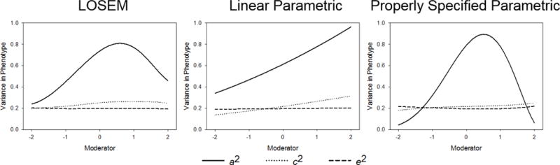
Average model parameters for LOSEM, a linear parametric model (mis-specified), and a properly specified parametric model. All datasets included 1000 twin pairs.

Power to detect G×E interaction was high in each case. Power was greater than 80% for each of the polynomial terms used in the properly specified parametric model, implying that the complex functional form was necessary to accurately describe the data. Power was also high for the improperly specified linear parametric term (87%). Although this model successfully detected the general increase in genetic effects, exclusive reliance on levels of significance misleads conclusions about the actual functional form of the interaction. Consistent with earlier results, LOSEM was slightly more conservative than the parametric approach (power = 78%), but offers a flexible view of the interaction.

Recommendations for Employing LOSEM

In this section, we offer initial recommendations on effective ways to use the LOSEM approach to inform studies of G×E interaction.

Define the research range of interest for the moderator

In the context of statistical moderation, the research range of interest refers to (and is confined to) the span of the moderator for which data are available (Roisman et al., 2012). For example, the plots in Figure 3 are based on a research range of interest between - 2 SD and + 2 SD of SES, a region that contains nearly all of the empirical observations and does not extend to regions of no data availability. Using a parametric approach, it would be analytically feasible to explore the range from −8 SD to −4 SD of moderators such as SES, but this range extrapolates well beyond the empirical data. Similarly, applying LOSEM trends identified where data density is sufficient to regions that have not been sampled adequately would be suspect. Researchers should, of course, take care to interpret results based on sufficient data and report on their moderator in reference to a general standard (i.e., whether the moderator spans from bad to normal, such as child maltreatment to no child maltreatment, or from poor to good, such as is the case for most standardized measures of SES in representative samples).

Get the main effects right

Just as the parametric G×E approach requires that the shape of the interaction effect conform to a parametric function, it also requires that the main effect of the moderator conform to a parametric function; the means model (“main effect”) is also capable of being nonlinear in ways that parametric methods typically do not attempt to model (Rathouz, 2008). Prior to interpreting interaction effects estimated using parametric and LOSEM approaches, it is therefore important to scrutinize whether the means models are consistent across the two methods. If these effects on the mean differ, the interaction component may also differ, as the biometric components (and biometric interactions) in both approaches model phenotypic variance that is unique of the moderator. In a situation in which the main effects from the two approaches are not in close agreement, one should use the function capturing the LOSEM mean effect (column 3 of Figure 3 and column H of Supplementary File 2) to residualize the phenotype prior to implementing the parametric model (now with the means model set to zero). This would enable parametric and nonparametric modeling of ACE component variance on the same residuals, allowing direct comparisons between the two approaches to be made. Alternatively, the parametric specification of the effect of the moderator on the phenotype may be expanded to more closely capture the nonparametric trend, but in certain circumstances this may prove difficult.

Choose the right baseline model

Standard approaches to model fitting/trimming (e.g., Neale et al., 1989) can guide the selection of reduced biometric models (e.g., an AE model over an ACE model) or an alternative model (e.g., one including D rather than C variance components). In the case of LOSEM, the possibility exists for reducing or otherwise varying models differently at each target value of the moderator. Such locally-distinct genetic architectures are unlikely to have biological validity. Different genetic architectures would imply mechanisms that exist in the organism exerting not just varying influence on the phenotype, but are actually absent at some levels of the moderator. For this reason, we recommend that the same variance components be modeled at all levels of the moderator, with differences in magnitude being the primary focus. Still, it is conceivable that there are highly complex processes at play that give rise to a situation, for example, in which dominant genetic influences on a phenotype are only manifest at certain levels of a moderator. Ultimately, this is a data- and topic-specific question, and the near-endless modeling possibilities must be tempered by the principle of parsimony.

Choose the right tool from the toolkit

The major advantage of using a nonparametric exploratory approach, such as LOSEM, is the ability to detect (or to rule out) nonlinear G×E interactions. In the current application of LOSEM, we detected model mis-specification for kindergarten reading ability and corrected this by applying a more appropriate interaction function (Figure 4). This pattern is very easily noticed when nonparametric approaches are used to inform model selection. Of course, additional data are necessary to evaluate the replicability of the nonlinearity, which was only observed for one measure (reading) and at one developmental period (Kindergarten). It is unclear whether other G×E interaction studies may have reported biased results simply due to inappropriate statistical models. Incorporating flexible, nonparametric approaches as a data analytic step can help avoid such pitfalls.

We simulated one hypothetical example in which this pitfall occurred. LOSEM and a properly specified parametric model correctly identified a highly complex relation between the moderator and genetic variance (see Figure 7). A linear specification of G×E interaction did not identify this trend. Of course, investigators could add polynomial terms to their parametric functions ad infinitum in an attempt to capture all the complexity found in the data. This process most likely will prove computationally infeasible as even models incorporating second-order polynomial terms are known to be “sensitive to starting values and prone to local minima…Care must be taken when fitting these models” (Purcell, 2002, p. 562). Because LOSEM relies on a very simple structural model, such concerns are minimized, and LOSEM results can intelligently guide parametric model fitting.

Examine differences in the magnitude of variance across meaningful ranges of the moderator and the proportion affected

To supplement basic visual inspection of LOSEM trends, differences in the magnitudes of variance offers a convenient way to quantify how quickly genetic or environmental influences shift over meaningful levels of the moderator. For example, Table 1 demonstrates how this approach can help guide interpretation of trends. Further, Roisman et al. (2012) suggested calculating the “proportion affected” when evaluating the shape and importance of candidate G×E interaction results. Individuals are “affected” by the interaction if they experience a level of the environment beyond the crossover point of a candidate G×E interaction (i.e., the point of the moderator at which two genotypes appear equivalent on a phenotype). The region beyond this point indicates that genotypes respond differently to the environment. They argued that if 16% or 2% of the sample falls above this point, then that would provide good or speculative evidence, respectively, for the practical importance of an interaction effect. This convention was suggested based on reference to a normal distribution in which 16% and 2% of the sample would be 1 and 2 SD above the mean, respectively. In the current context, the spike in genetic variance for age 4 math occurs at SES of +1.5 SD, indicating that approximately 7% of the sample is “affected” by the spike. By this criterion, evidence for this increase in genetic variance might be termed meaningful in magnitude (i.e., accounting for approximately half of the total increase in genetic variance, see Table 1) on a meaningful proportion of the sample.

Use permutation tests as a conservative inferential guide to modeling G×E

Generally, nonparametric models are less efficient than parametric models when the underlying functional form is truly parametric (Eubank, 1999, p. 9; Hart, 1997, p. 1; Horowitz, 2009, p. 6). If investigators do not have prior knowledge of the exact form a G×E interaction takes, however, it is unclear which approach will prove more powerful. Based on the current results, LOSEM is able to detect statistically significant G×E interaction and offer a flexible vantage point of the functional form that is not constrained by limited prior knowledge. Permutation tests offer a critical piece of information to guide statistical inferences, but descriptive applications of LOSEM to explore data may prove more useful pragmatically. We encourage other investigators to improve or expand on the nonparametric tests proposed in this manuscript. Currently, we are pursuing applications that take into account model fit (i.e., χ²), or that are locally-sensitive, rather than providing an omnibus test of G×E interaction.

Conclusions and Future Directions

We have demonstrated the utility of a novel approach to analyzing G×E interaction results. LOSEM produces flexible nonparametric estimates of G×E interaction trends that can detect nonlinearities and inform subsequent confirmatory model fitting. We applied this approach to a highly studied effect with widely used data to make novel insights concerning trends found in the data. We plotted nonparametric estimates of genetic, shared environmental, and nonshared environmental variance across levels of SES in the ECLS-B sample for six cognitive ability phenotypes. Using the LOSEM approach, we detected an inverted-U shape curve for the genetic variance of kindergarten reading ability. Following up this approach with a standard parametric model that included a quadratic term (Purcell, 2002), we confirmed that this nonlinearity was statistically significant. As mentioned previously, this result for a single phenotype at a single age requires additional replication and investigation before it can inform theory, but the process of discovery represents a key strength of LOSEM.

Additionally, we used the flexible LOSEM results to probe where in the SES distribution the majority of the differences in magnitude of genetic variance occur. For several phenotypes, the majority of the G×SES interaction occurred in the transition from somewhat low SES to somewhat high SES environments with almost no increase associated with the high to very high SES range. Again, this trend would be completely missed if relying solely on parametric, linear models. Of course, the current study is primarily concerned with displaying the utility of the novel LOSEM approach for G×E interaction studies. Much more empirical evidence will be needed to evaluate the exact functional form of this interaction across different ages and cognitive phenotypes.

As with all exploratory approaches, LOSEM has potential pitfalls. Exploratory data analysis opens up researcher degrees of freedom that might allow for inappropriate manipulation of data to capitalize on noise (Simmons et al., 2011). For example, LOSEM results could be used to find just the “right” points of the moderator to dichotomize or categorize different groups. A related pitfall would be to over-interpret minor deviations of the LOSEM trends as meaningful effects. We have provided some recommendations for avoiding this pitfall, such as using the proportion affected by the trend, using a conservative permutation test for nonparametric G×E interaction, and following LOSEM analyses with confirmatory approaches.

Interpretation of LOSEM must balance the detection of meaningful nuance from random noise. This balance is primarily determined by the bw parameter. When this parameter is increased, noise in the estimates is reduced, but more nuanced micro-trends may be missed. When shrunk, the estimates conform closely to local subsets of the data, thus increasing the capability to pick up on nuanced trends, but also increasing the chance of picking up on statistical noise. This tradeoff is inherent in kernel regression methodology (Hart, 1997, p. 12; Li & Racine, 2007). We have followed the recommendation of Hildebrandt et al. (2009) in calculating bw based on the sample size and standard deviation of the moderator. As discussed extensively in previously published work on nonparametric regression methods, a number of other data driven methods exist for choosing the optimal bw (Bowman, 1984; Rudemo, 1982; Hurvich et al., 1998), along with adaptive bandwidth approaches, in which local estimates are weighted by a constant number of nearby datapoints. Each of these methods may provide slightly different values for bw and therefore possibly produce substantively different trend estimates. Additionally, we followed Hildebrandt et al. (2009) in recommending the kernel function follow a Gaussian distribution, but a number of other functional forms are available. Generally, alternative kernel forms do not impact substantive conclusions, especially compared to the more important choice of bw (Eubank, 1999, p. 177).

A major limitation of the LOSEM approach is that it requires the environmental moderator to be measured at the family-level. Quantitative behavior genetic methods use the sibling pair as the unit of analysis, and the weighting function must be applied at this level. Therefore, the LOSEM approach, in its current form, is unable to estimate G×E for moderators that vary within families. Several papers have developed and scrutinized parametric G×E methods for moderators that vary within families (Rathouz et al., 2008; van Hulle et al., 2013; van der Sluis et al., 2012), which allow for modeling of gene-environment correlation. Future efforts to develop LOSEM methods to handle such data structures would be highly valuable.

In conclusion, LOSEM can be a valuable tool in the behavior genetic toolkit for probing G×E interactions. As researchers have successfully adopted LOESS approaches to regression to explore and visualize data, LOSEM can be applied to behavior genetic data to detect nonlinearities or discontinuities of trends that would otherwise be missed. In the online supplement, we provide scripts for implementing LOSEM in Mplus and in OpenMx. We encourage researchers to apply LOSEM to better understand the complex interplay between genetic and environmental influences.

References

- Asparouhov T. Sampling weights in latent variable modeling. Struct Equ Modeling. 2005;12(3):411–434. [Google Scholar]
- Benjamin Y, Hochberg Y. Controlling the false discovery rate: A practical and powerful approach to multiple testing. J R Stat Soc Series B Stat Methodol. 1995;57(1):289–300. [Google Scholar]
- Boker S, Neale M, Maes H, Wilde M, Spiegel M, Brick T, Fox J. OpenMx: An open source extended structural equation modeling framework. Psychometrika. 2011;76:306–317. doi: 10.1007/s11336-010-9200-6. [DOI] [PMC free article] [PubMed] [Google Scholar]
- Bowman AW. An alternative method of cross-validation for the smoothing of density estimates. Biometrika. 1984;71:353–360. [Google Scholar]
- Briley DA, Harden KP, Tucker-Drob EM. Genotype × cohort interaction on completed fertility and age at first birth. Behav Genet. 2015;45:71–83. doi: 10.1007/s10519-014-9693-3. [DOI] [PMC free article] [PubMed] [Google Scholar]
- Bronfenbrenner U, Ceci SJ. Nature-nurture reconceptualized in developmental perspective: A bioecological model. Psychol Rev. 1994;101:568–586. doi: 10.1037/0033-295x.101.4.568. [DOI] [PubMed] [Google Scholar]
- Burt SA, McGue M, DeMarte JA, Krueger RF, Iacono WG. Timing of menarche and the origins of conduct disorder. Arch Gen Psychiatry. 2006;63(8):890–896. doi: 10.1001/archpsyc.63.8.890. [DOI] [PMC free article] [PubMed] [Google Scholar]
- Cleveland WS, Devlin SJ. Locally-weighted regression: An approach to regression analysis by local fitting. J Am Stat Assoc. 1988;83(403):596–610. [Google Scholar]
- Eubank RL. Nonparametric regression and spline smoothing. 2nd. Dekker; New York, NY: 1999. [Google Scholar]
- Fox J. Nonparametric simple regression: Smoothing scatterplots. 2000. (Sage University Papers Series on Quantitative Applications in the Social Sciences, 07-130). [Google Scholar]
- Gasser T, Gervini D, Molinari L. Kernel estimation, shape-invariant modeling and structural analysis. In: Hauspie R, Cameron N, Molinari L, editors. Methods in human growth research. Cambridge University Press; 2004. pp. 15–33. [Google Scholar]
- Good P. Permutation, parametric, and bootstrap tests of hypotheses. 3rd. Springer; New York, NY: 2005. [Google Scholar]
- Green PJ, Silverman BW. Nonparametric regression and generalized linear models: A roughness penalty approach. Chapman & Hall; London, UK: 1994. [Google Scholar]
- Hallquist M. MplusAutomation: Automating Mplus model estimation and interpretation. R package version 0.5 2011 [Google Scholar]
- Hart JD. Nonparametric smoothing and lack-of-fit tests. Springer; New York, NY: 1997. [Google Scholar]
- Hildebrandt A, Wilhelm O, Robitzsch A. Complementary and competing factor analytic approaches for the investigation of measurement invariance. Rev Psychol. 2009;16(2):87–102. [Google Scholar]
- Horowitz JL. Semiparametric and nonparametric methods in econometrics. Springer; New York, NY: 2009. [Google Scholar]
- Hülür G, Wilhelm O, Robitzsch A. Intelligence differentiation in early childhood. J Individ Differ. 2011;32(3):170–179. [Google Scholar]
- Huvich CM, Simonoff JS, Tsai C-L. Smoothing parameter selection in nonparametric regression using an improved Akaike information criterion. J R Stat Soc Series B Methodol. 1998;60:271–293. [Google Scholar]
- Johnson W. Genetic and environmental influences on behavior: capturing all the interplay. Psychol Rev. 2007;114(2):423–440. doi: 10.1037/0033-295X.114.2.423. [DOI] [PubMed] [Google Scholar]
- Kirkpatrick R, McGue M, Iacono WG. Replication of a gene-environment interaction via multimodel inference: Additive-genetic variance in adolescents’ general cognitive ability increases with family-of-origin socioeconomic status. Behav Genet. 2015;45:200–214. doi: 10.1007/s10519-014-9698-y. [DOI] [PMC free article] [PubMed] [Google Scholar]
- Li Q, Racine J. Nonparametric econometrics: Theory and practice. Princeton University Press; 2007. [Google Scholar]
- Logan JAR, Petrill SA, Hart SA, Schatschneider C, Thompson LA, Deater-Deckard K, DeThorne LS, Bartlett C. Heritability across the distribution: An application of quantile regression. Behav Genet. 2012;42:256–267. doi: 10.1007/s10519-011-9497-7. [DOI] [PMC free article] [PubMed] [Google Scholar]
- Medland SE, Neale MC, Eaves LJ, Neale BM. A note on the parameterization of Purcell’s G× E model for ordinal and binary data. Behav Genet. 2009;39(2):220–229. doi: 10.1007/s10519-008-9247-7. [DOI] [PMC free article] [PubMed] [Google Scholar]
- Mendle J, Moore SR, Briley DA, Harden KP. Puberty, socioeconomic status, and depressive symptoms in adolescent girls: Evidence for genotype × environment interactions. Clin Psychol Sci. 2015 doi: 10.1177/2167702614563598. [DOI] [PMC free article] [PubMed] [Google Scholar]
- Molenaar D, Dolan CV. Testing systematic genotype by environment interactions using item level data. Behav Genet. 2014;44:212–231. doi: 10.1007/s10519-014-9647-9. [DOI] [PubMed] [Google Scholar]
- Muthén LK, Muthén BO. Mplus user’s guide. 6th. Los Angeles, CA: Muthén and Muthén; 1998–2010. [Google Scholar]
- Neale MC, Heath AC, Hewitt JK, Eaves LJ, Fulker DW. Fitting genetic models with LISREL: Hypothesis testing. Behav Genet. 1989;19(1):37–49. doi: 10.1007/BF01065882. [DOI] [PubMed] [Google Scholar]
- Neale MC, Maes HHM. Methodology for genetic studies of twins and families. Dordrecht, The Netherlands: Kluwer Academic Publishers; 2005. [Google Scholar]
- Plomin R, DeFries DC, Loehlin JC. Genotype-environment interaction and correlation in the analysis of human behavior. Psychol Bull. 1977;84(2):309–322. [PubMed] [Google Scholar]
- Price TS, Jaffee SR. Effects of the family environment: gene-environment interaction and passive gene-environment correlation. Dev Psychol. 2008;44(2):305–315. doi: 10.1037/0012-1649.44.2.305. [DOI] [PubMed] [Google Scholar]
- Purcell S. Variance components models for gene-environment interaction in twin analysis. Twin Res. 2002;5:554–571. doi: 10.1375/136905202762342026. [DOI] [PubMed] [Google Scholar]
- R Development Core Team. R: A language and environment for statistical computing. R Foundation for Statistical Computing; Vienna, Austria: 2013. URL http://www.R-project.org/ [Google Scholar]
- Racine J. Consistent significance testing for nonparametric regression. J Bus Econ Stat. 1997;15(3):369–378. [Google Scholar]
- Rathouz PJ, Van Hulle CA, Rodgers JL, Waldman ID, Lahey BB. Specification, testing, and interpretation of gene-by-measured-environment interaction models in the presence of gene–environment correlation. Behav Genet. 2008;38(3):301–315. doi: 10.1007/s10519-008-9193-4. [DOI] [PMC free article] [PubMed] [Google Scholar]
- Rhemtulla M, Tucker-Drob EM. Gene-by-socioeconomic status interaction on school readiness. Behav Genet. 2012;42:549–558. doi: 10.1007/s10519-012-9527-0. [DOI] [PMC free article] [PubMed] [Google Scholar]
- Roisman GI, Newman DA, Fraley RC, Haltigan JD, Groh AM, Haydon KC. Distinguishing differential susceptibility from diathesis-stress: Recommendations for evaluating interaction effects. Dev Psychopathol. 2012;24:389–409. doi: 10.1017/S0954579412000065. [DOI] [PubMed] [Google Scholar]
- Rudemo M. Empirical choice of histograms and kernel density estimates. Scand Stat Theory Appl. 1982;9:65–78. [Google Scholar]
- Scarr S. Developmental theories for the 1990s: Development and individual differences. Child Dev. 1992;63:1–19. [PubMed] [Google Scholar]
- Schroeders U, Schipolowski S, Wilhelm O. Age-related changes in mean and covariance structure of fluid and crystallized intelligence in childhood and adolescence. Intell. 2015;48:15–29. [Google Scholar]
- Schwabe I, van den Berg SM. Assessing genotype by environment interaction in case of heterogeneous measurement error. Behav Genet. 2014 doi: 10.1007/s10519-014-9649-7. Advance online publication. [DOI] [PubMed] [Google Scholar]
- Simmons JP, Nelson LD, Simonsohn U. False-positive psychology: Undisclosed flexibility in data collection and analysis allows presenting anything as significant. Psychol Sci. 2011;22:1359–1366. doi: 10.1177/0956797611417632. [DOI] [PubMed] [Google Scholar]
- Snow K, Derecho A, Wheeless S, Lennon J, Rosen J, Rogers J, Einaudi P. Early Childhood Longitudinal Study, Birth Cohort (ECLS-B), kindergarten 2006 and 2007 data file user’s manual (2010–010) Washington, DC: U.S. Department of Education, National Center for Education Statistics, Institute of Education Sciences; 2009. [Google Scholar]
- Takezawa K. Introduction to nonparametric regression. Wiley; Hoboken, NJ: 2006. [Google Scholar]
- Tucker-Drob EM. Preschools reduce early academic achievement gaps: A longitudinal twin approach. Psychol Sci. 2012;23:310–319. doi: 10.1177/0956797611426728. [DOI] [PMC free article] [PubMed] [Google Scholar]
- Tucker-Drob EM, Briley DA, Harden KP. Genetic and environmental influences on cognition across development and context. Curr Dir Psychol Sci. 2013;22:349–355. doi: 10.1177/0963721413485087. [DOI] [PMC free article] [PubMed] [Google Scholar]
- Tucker-Drob EM, Harden KP. Learning motivation mediates gene-by-socioeconomic status interaction on early mathematics achievement. Learn Individ Differ. 2012;22:37–45. doi: 10.1016/j.lindif.2011.11.015. [DOI] [PMC free article] [PubMed] [Google Scholar]
- Tucker-Drob EM, Rhemtulla M, Harden KP, Turkheimer E, Fask D. Emergence of gene-by-socioeconomic status interaction on infant mental ability between 10 months and 2 years. Psychol Sci. 2011;22:125–133. doi: 10.1177/0956797610392926. [DOI] [PMC free article] [PubMed] [Google Scholar]
- Turkheimer E, Gottesman II. Individual differences and the canalization of human behavior. Dev Psychol. 1991;27:18–22. [Google Scholar]
- Turkheimer E, Horn EE. Interactions between socioeconomic status and components of variation in cognitive ability. In: Finkel D, Reynolds CA, editors. Behavior genetics of cognition across the lifespan. New York: Springer; 2014. pp. 41–68. [Google Scholar]
- van der Sluis S, Posthuma D, Dolan CV. A note on false positives and power in G×E modelling of twin data. Behav Genet. 2012;42(1):170–186. doi: 10.1007/s10519-011-9480-3. [DOI] [PMC free article] [PubMed] [Google Scholar]
- van Hulle CA, Lahey BB, Rathouz PJ. Operating characteristics of alternative statistical methods for detecting gene-by-measured environment interaction in the presence of gene–environment correlation in twin and sibling studies. Behav Genet. 2013;43(1):71–84. doi: 10.1007/s10519-012-9568-4. [DOI] [PMC free article] [PubMed] [Google Scholar]
- Zheng H, Rathouz PJ. Fitting procedures for novel gene-by-measured environment interaction models in behavior genetic designs. Behav Genet. 2015 doi: 10.1007/s10519-015-9707-9. Advanced online publication. [DOI] [PMC free article] [PubMed] [Google Scholar]
Associated Data
This section collects any data citations, data availability statements, or supplementary materials included in this article.