The Predicted Cross Value for Genetic Introgression of Multiple Alleles

Han et al. introduce a new metric, the Predicted Cross Value (PCV), for selecting breeding parents. Unlike estimated breeding values, which represent...

Abstract

We consider the plant genetic improvement challenge of introgressing multiple alleles from a homozygous donor to a recipient. First, we frame the project as an algorithmic process that can be mathematically formulated. We then introduce a novel metric for selecting breeding parents that we refer to as the predicted cross value (PCV). Unlike estimated breeding values, which represent predictions of general combining ability, the PCV predicts specific combining ability. The PCV takes estimates of recombination frequencies as an input vector and calculates the probability that a pair of parents will produce a gamete with desirable alleles at all specified loci. We compared the PCV approach with existing estimated-breeding-value approaches in two simulation experiments, in which 7 and 20 desirable alleles were to be introgressed from a donor line into a recipient line. Results suggest that the PCV is more efficient and effective for multi-allelic trait introgression. We also discuss how operations research can be used for other crop genetic improvement projects and suggest several future research directions.

DISCOVERIES of genetic variants associated with crop phenotypic variants have been accelerating through use of forward and reverse genetics approaches. We now have databases cataloging thousands of genetic variants (alleles) associated with desirable phenotypes in large germplasm repositories (McCouch et al. 2012; Cavanagh et al. 2013). This information tells us that desirable alleles are distributed unevenly throughout germplasm collections and unevenly across crop genomes. Nonetheless, these resources will provide desirable alleles for genetic improvement of crops in rapidly changing environments (Kumar et al. 2010; Leung et al. 2015).

Introgression of a single desirable allele from an inferior agronomic cultivar to an elite cultivar is routinely accomplished using marker-assisted backcrossing strategies (Visscher et al. 1996; Frisch et al. 1999; Frisch and Melchinger 2005; Peng et al. 2014a). Furthermore, as long as there are very few cultivars that are capable of maintenance and regeneration in tissue culture, creation of novel alleles through genome-editing technologies will likewise depend on trait introgression for cultivar development. Introgression of multiple alleles is not as well studied, but genomic selection (Bernardo 2009; Longin and Reif 2014; Gorjanc et al. 2016) and marker-assisted gene pyramiding (Servin et al. 2004; Canzar and El-Kebir 2011; Xu et al. 2011; De Beukelaer et al. 2015) have been proposed as approaches for introgressing multiple alleles from unadapted landraces into elite cultivars.

The genomic estimated breeding value (GEBV) (Meuwissen et al. 2001), based on large sets of genomic markers, is commonly used for parental selection and has been proposed for trait introgression projects in crop species (Bernardo 2009). The optimal haploid value (OHV) (Daetwyler et al. 2015) was proposed as an alternative breeding value metric to evaluate potential rather than a realized breeding value among progeny. Both of these metrics may be thought of as predictors of general combining ability for an inference space consisting of a breeding population. Prior to development of the GEBV, van Berloo and Stam (1998) proposed a combination index (CI) to identify pairs of recombinant inbred lines (RILs) derived from a single mating of two homozygous lines for purposes of accumulating desirable QTL in subsequent generations of breeding. Their CI metric may be thought of as a predictor of specific combining ability among sets of RILs within the family derived from the initial cross. While the CI was evaluated in simulated genomes with various degrees of linkage disequilibrium (LD) among QTL, none of these metrics explicitly use recombination or linkage phase information. Recently, Bonk et al. (2016) developed breeding value models for dairy herds that use linkage map information to identify matings that will produce progeny with large variances of breeding values. The premise of this approach was that a higher Mendelian sampling variance for a given pair of parents would lead to a higher chance to generating outstanding progeny with many desirable alleles.

Herein, we build on the concepts introduced by van Berloo and Stam (1998) as well as those of Bonk et al. (2016) and propose a metric, the predicted cross value (PCV) for selecting specific crosses. We apply the PCV to the process of introgressing multiple alleles from a single homozygous donor. However, rather than applying the metric to RILs derived from a single cross, we apply it to any arbitrary set of progeny derived from crosses in multiple generations which is required for introgressing multiple alleles from a donor. The PCV is a predictor of specific combining ability for an inference space consisting of future sets of progeny derived from possible crosses in a breeding population. Explicitly, the PCV calculates the probability that a cross will produce an ideal genotype in two future generations of matings.

We compare selection using PCV with GEBV and OHV in two multi-allelic introgression projects: (a) Introgression of seven independently segregating alleles. Such situations occur when the goal is to adapt a tropical cultivar to high latitudes for purposes of evaluating other agronomic traits without confounding influences of maturity. (b) Introgression of 20 alleles from an exotic accession into an elite cultivar for purposes of improving a polygenic trait.

Methods

Formulation

The general objective of multi-allelic introgression projects is to transfer multiple desirable alleles, or haplotypes, from a donor to a recipient. The ultimate goal is to produce at least one individual with a genome consisting of homozygous desirable haplotypes and no undesirable alleles from the donor. The introgression process begins by identifying the donor and recipient cultivars based on criteria defined by the breeder. The selected cultivars are then planted, grown to sexual maturity, and crossed. The resulting seeds are harvested and planted along with the recipient parent. The progeny are evaluated to assure that they represent the F₁ generation with half of their genomes inherited from each parent. In subsequent filial generations, breeding parents are selected from the current population to be crossed, and the progeny are evaluated to determine if any meet the goal. If not, the process of selection and reproduction will be repeated.

Multi-allelic introgression as an algorithmic process:

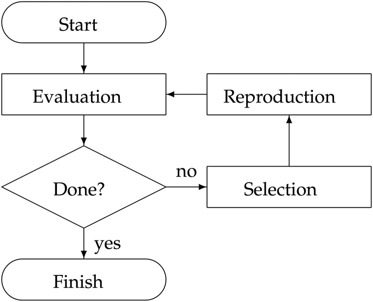
We illustrate the major components of the introgression process in Figure 1 and explain each of the components as follows.

Figure 1.

Flowchart of the multi-allelic introgression process.

The point:

The introgression process starts with identification of at least one recipient and one donor. In the case of most annual crops, both recipient and donor are homozygous throughout their genomes. The majority of alleles in the recipient are desirable but some are undesirable. The donor carries the desirable versions of alleles that the recipient is lacking, but the rest of the alleles of the donor are undesirable.

The step:

In this step, marker genotypes of individuals in the current generation are evaluated.

The condition:

The stopping condition is checked in this step, which determines whether the current generation of progeny contains an individual that is homozygous with only desirable alleles from both the recipient and donor.

The step:

In this step, breeding parents are selected from the current generation of individuals to produce the next generation of progeny. The current generation includes the recipient line and the newly produced generation of progeny but not individuals from previous generations. This is because the recipient is a replicable entity, whereas individual progeny from previous generations have lived through their life cycle and were not replicable. If the cross involves the recipient cultivar, then it is referred to as a backcross. Another special case of selection is to select only one plant to cross through self-pollination.

The step:

In this step, the breeding parents selected from the selection step are crossed to produce a new generation of progeny. The genotypes of this next generation of progeny are produced through the stochastic processes of transmission genetics.

The point:

The goal of an introgression breeding project is to produce an ideal line that inherits only the desirable alleles from the recipient and the donor line. In other words, the ideal line is homozygous and does not contain undesirable alleles. The breeding process finishes when an ideal line has been produced. This line will then proceed to further stages of cultivar development.

Simplifying assumptions:

Several assumptions are made to simplify the formulation and illustrate the core elements of the process. In the Discussion section, we discuss relaxing these assumptions in future studies.

1. Consider annual diploid and allopolyploid species such as corn, sorghum, sunflower, rice, and wheat with subgenome-specific loci.

2. Consider a single multi-allelic trait, where all segregating loci associated with the trait are known. Results also apply to multiple traits such as gene stacks where all traits are of equal value.

3. All marker alleles are either desirable or undesirable. Values of alleles could be modeled as continuous from some distribution or, in many cases, the value of an allele is unknown.

4. To illustrate the principles, all desirable alleles missing in the recipient are carried by one donor line.

5. One pair of parents is selected for crossing in each generation, with self-pollination as a special but feasible option. In actual breeding practice, multiple crosses are sometimes made to produce sufficient numbers of progeny for field trial evaluations.

6. During evaluation, a sufficient number of informative markers are distributed throughout the genome at sufficient density to allow estimation of recombination between all adjacent pairs of markers.

7. Recombination events between pairs of adjacent loci are assumed to be independent (Haldane 1919).

Mathematical formulation of the multi-allelic introgression process:

We use an N-by-two binary matrix, say $L\in {\mathbb{B}}^{N\times 2},$ to represent the genotype of an individual plant, where N is the total number of QTL in the genome. Each row represents a locus in the genome, and the two columns represent the paired chromosomes. The binary value $L_{i,j}$ indicates whether the allele in locus i of chromosome j is desirable $\left(L_{i,j}=1\right)$ or undesirable $\left(L_{i,j}=0\right).$

Definition 0.1. We define the gamete function, $g=\text{Gamete}\left(L,J\right),$ as follows. Its input parameters include a binary matrix $L\in {\mathbb{B}}^{N\times 2}$ and a binary vector $J\in {\mathbb{B}}^N.$ Its output is a binary vector $g\in {\mathbb{B}}^N,$ which is determined as $g_i=L_{i,J_i+1},\forall i\in \left\{1,\dots ,N\right\}.$

In this definition, L represents the genotype of an individual plant, and the binary vector J indicates the sources of inheritance for the alleles in a gamete. If $J_i=0,$ then the $g_i$ allele is inherited from $L_{i,1};$ otherwise it originates from $L_{i,2}.$ To realistically represent the actual gamete formation process, the input binary vector J must be a random one following a special distribution, which is defined as follows.

Definition 0.2. We say that the random binary vector $J\in {\mathbb{B}}^N$ follows an inheritance distribution with parameter vector $r\in {\left[0,0.5\right]}^{N-1}$ if

$$J_1=\{\begin{array}{lll}0\hfill & \text{w}.\text{p}.\hfill & 0.5\hfill \\ 1\hfill & \text{w}.\text{p}.\hfill & 0.5\hfill \end{array},$$ (1)

$$J_i=\{\begin{array}{ccc}{J}_{i-1}& \text{w}.\text{p}.& 1-r_{i-1}\\ 1-J_{i-1}& \text{w}.\text{p}.& r_{i-1}\end{array},\forall i\in \left\{2,\dots ,N\right\}.$$ (2)

Here, “w.p.” stands for “with probability.”

According to Mendel’s second law, $L_{1,1}$ and $L_{1,2}$ are equally likely to transmit $g_1,$ hence Equation 1. Given the inheritance source of the allele $\left(i-1\right)$ in the gamete, the probability that allele i comes from the same chromosome $\left(J_i=J_{i-1}\right)$ is $1-r_{i-1},$ which explains Equation 2.

Definition 0.3. We define the reproduce function, $X=\text{Reproduce}\left(L^1,L^2,r,K\right),$ as follows. Its input parameters include two binary matrices $L^1,L^2\in {\mathbb{B}}^{N\times 2},$ a vector $r\in {\left[0,0.5\right]}^{N-1},$ and a positive integer number K. Its output is a three-dimensional matrix $X\in {\mathbb{B}}^{N\times 2\times K},$ representing a population of K progeny, which is determined by first generating $2K$ independent and identically distributed random vectors from the inheritance distribution with parameter vector r, denoted as $J_p,\forall p\in \left\{1,\dots ,2K\right\},$ and then setting $X_{i,j,k}={\text{Gamete}}_i\left(L^j,J_{2k-2+j}\right),\forall i\in \left\{1,\dots ,N\right\},j\in \left\{1,2\right\},k\in \left\{1,\dots ,K\right\}.$

Definition 0.4. The select function, $\left[k_1,k_2\right]=\text{Select}\left(X,r\right),$ is defined as follows. Its input parameters include a three-dimensional binary matrix, $X\in {\mathbb{B}}^{N\times 2\times K},$ and a vector $r\in {\left[0,0.5\right]}^{N-1}.$ Its output includes two integers, $k_1,k_2\in \mathbb{Z}\mathrm{.}$

Here, $k_1$ and $k_2$ are the indices of the selected parents in the breeding population X. If $k_1=k_2,$ then self-pollination is suggested as the breeding strategy.

Definition 0.5. We define the breed function as $G=\text{Breed}\left(P^0,r,K\right).$ Its input parameters include a three-dimensional binary matrix $P^0\in {\mathbb{B}}^{N\times 2\times 2},$ a vector $r\in {\left[0,0.5\right]}^{N-1},$ and a positive integer K. Its output, G, is the number of generations it takes to successfully finish the process, which is determined through the following steps.

Step 0 (initialization). Set $t=0$ and go to step 1.

Step 1 (evaluation). If$\underset{k}{\max }\left\{{\displaystyle \sum _{i=1}^N\left(P_{i,1,k}^t+P_{i,2,k}^t\right)}\right\}=2N$

RETURN: $G=t.$

Else go to step 2.

Step 2 (selection). Obtain $\left[k_1^t,k_2^t\right]=\text{Select}\left(P^t,r\right)$ and go to step 3.

Step 3 (reproduction). Obtain $P^{t+1}=$$\text{Reproduce}\left(P_{:,:,k_1^t}^t,P_{:,:,k_2^t}^t,r,K\right),$ update $t\leftarrow t+1,$ and go to step 1.

The function $\text{Breed}\left(P^0,r,K\right)$ is a mathematical formulation of the multi-allelic introgression process, in which the selection step has the most significant influence on the efficiency of the process. In Existing approaches for parental selection, we review existing approaches for parental selection, and then we propose a new approach in PCV for parental selection.

Existing approaches for parental selection:

The GEBV approach selects breeding parents based on the GEBV. In the context of multi-allelic introgression, if we assume uniform weight for all desirable alleles, then the GEBV of an individual L is equivalent to the number of desirable alleles:

$${\displaystyle \sum _{i=1}^N\left(L_{i,1}+L_{i,2}\right)}.$$ (3)

The two individuals with the highest GEBV will be selected according to the GEBV approach.

The OHV approach (Daetwyler et al. 2015) defined a different metric for parental selection. This approach recognizes that meiosis can produce gametes with recombined haplotype loci. The OHV of an individual can be interpreted as the best doubled-haploid progeny that could possibly be produced by selfing such individual. As such, OHV measures the potential breeding value of the individual’s progeny. In the context of multi-allelic introgression, the OHV of an individual L is defined as:

$${\displaystyle \sum _{i=1}^{N}2\max \left\{L_{i,1},L_{i,2}\right\}}.$$ (4)

The two individuals with the highest OHV will be selected according to the OHV approach.

PCV for parental selection

We propose a new parental-selection approach using the PCV, which is defined as follows.

Definition of PCV:

Let $L^1,L^2\in {\mathbb{B}}^{N\times 2}$ denote two breeding individuals, and let $\left[g^1,g^2\right]$ denote a random progeny of theirs, where $g^1=\text{Gamete}\left(L^1,J^1\right)$ and $g^2=\text{Gamete}\left(L^2,J^2\right)$ are gametes produced by $L^1$ and $L^2,$ respectively. When the progeny $\left[g^1,g^2\right]$ is crossed with another individual (or itself) in the next generation, it will produce a gamete, which we denote as $g^3=\text{Gamete}\left(\left[g^1,g^2\right],J^3\right).$ Here $J^1,$ $J^2,$ and $J^3$ are three independent and identically distributed random vectors following the inheritance distribution with parameter vector r.

Definition 0.6. For a given pair of individuals $L^1$ and $L^2,$ the PCV is defined as the probability that a gamete, $g^3,$ produced by a random progeny from crossing these two individuals, will consist only of desirable alleles:

$$\text{PCV}\left(L^1,L^2,r\right)=P\left(g_i^3=1,\forall i\in \left\{1,\dots N\right\}\right).$$

Here, r is the recombination frequency vector.

The rationale for the PCV definition is to calculate the probability that none of the undesirable alleles survives two generations of meiosis. The essence of this approach is to select breeding parents based on their likelihood to produce an ideal gamete by combining their desirable alleles.

The water-pipe algorithm for calculating PCV:

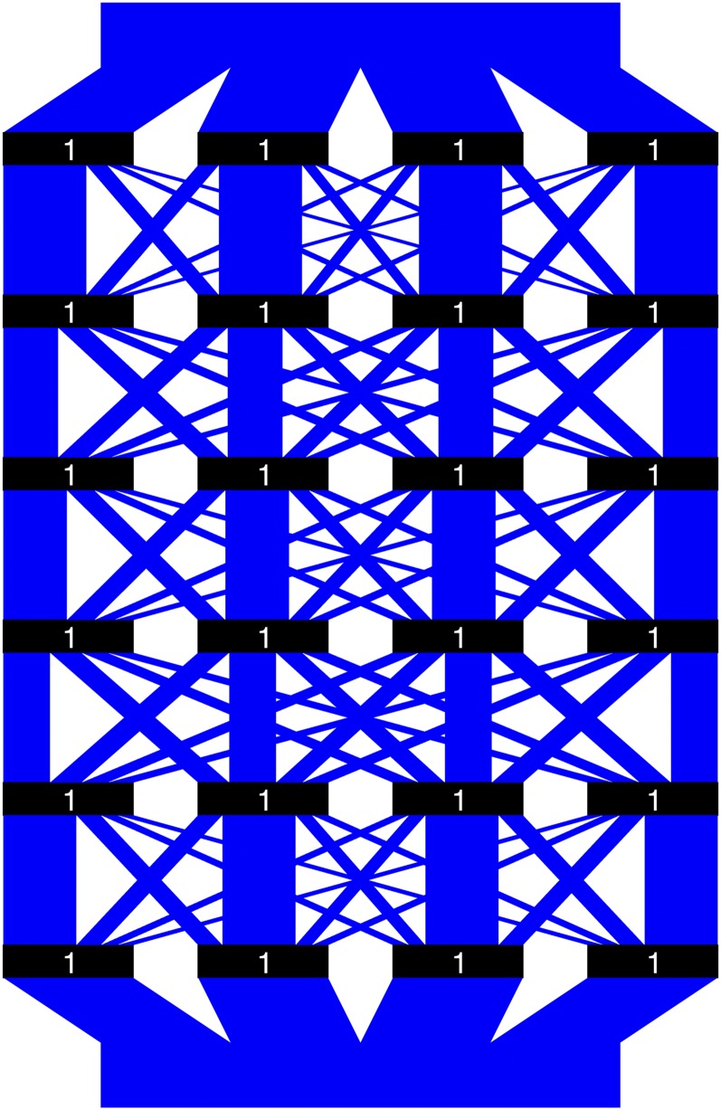
We designed a polynomial time algorithm for calculating PCV, which draws an analogy between conditional probabilities and water flows through a plumbing system. The plumbing system consists of N rows, four columns of valves, and a number of water pipes connecting them. The $4N$ valves correspond to the $4N$ alleles in the two breeding parents represented by the matrix $\left[L^1,L^2\right].$ For notational convenience, we will use $L\in {\mathbb{B}}^{N\times 4}$ to denote the matrix $\left[L^1,L^2\right],$ so $L_{i,1}=L_{i,1}^1,$ $L_{i,2}=L_{i,2}^1,$ $L_{i,3}=L_{i,1}^2,$ and $L_{i,4}=L_{i,2}^2$ for all $i\in \left\{1,\dots ,N\right\}.$ The intake on the top splits into four pipes with equal volumes leading to the four valves in the first row. Except for the four in the last row, each valve is connected by four pipes to the four valves in the next row. For all $i\in \left\{1,\dots ,N\right\}$ and $j\in \left\{1,2,3,4\right\},$ if allele $\left(i,j\right)$ is desirable, then the valve $\left(i,j\right)$ is open, and all the water that flows into the valve from above gets redistributed into the immediate downstream pipes according to their relative volumes and goes down to the next row; but if the allele $\left(i,j\right)$ is undesirable, then the valve $\left(i,j\right)$ is closed, and no matter how much water flows into the valve from above, the water is retained there, neither passing further down nor going back up. For all $i\in \left\{1,\dots ,N-1\right\},$ $j\in \left\{1,2,3,4\right\},$ and $k\in \left\{1,2,3,4\right\},$ the volume of the pipe that connects valves $\left(i,k\right)$ and $\left(i+1,j\right)$ is denoted as $T_{k,j,i},$ where T is a three-dimensional matrix, which is referred to as the transition matrix and defined as follows.

Definition 0.7. For a given vector of recombination frequencies, $r\in {\left[0,0.5\right]}^{N-1},$ the transition matrix $T\in {\left[0,0.5\right]}^{4\times 4\times \left(N-1\right)}$ is defined as

$$T_{:,:,i}=\left[\begin{array}{cccc}{\left(1-r_i\right)}^2& r_i\left(1-r_i\right)& 0.5r_i& 0.5r_i\\ r_i\left(1-r_i\right)& {\left(1-r_i\right)}^2& 0.5r_i& 0.5r_i\\ 0.5r_i& 0.5r_i& {\left(1-r_i\right)}^2& r_i\left(1-r_i\right)\\ 0.5r_i& 0.5r_i& r_i\left(1-r_i\right)& {\left(1-r_i\right)}^2\end{array}\right],$$

$$\forall i\in \left\{1,\dots ,N-1\right\}.$$ (5)

We define the water matrix $W\in {\left[0,1\right]}^{N\times 4}$ to represent the amount of water flowing inside the plumbing system. For all $i\in \left\{1,\dots ,N\right\}$ and $j\in \left\{1,2,3,4\right\},$ $W_{i,j}$ represents the amount of water that flows out of the jth valve in the ith row. This value can be interpreted as the probability that the first i alleles in the gamete $g^3$ are desirable and that the ith allele is inherited from the jth chromosome of the breeding parents.

Definition 0.8. We define the water matrix $W\in {\left[0,1\right]}^{N\times 4}$ as

$$W_{i,j}=P\left(g_1=\dots =g_i=1,g_i=L_{i,j}\right),\forall i\in \left\{1,\dots ,N\right\},j\in \left\{1,2,3,4\right\}.$$ (6)

Proposition 0.1. The water matrix can be calculated as follows.

$$W_{1,j}=\frac{1}{4}{L}_{1,j},\forall j\in \left\{1,2,3,4\right\},$$ (7)

$$W_{i,j}=L_{i,j}{\displaystyle \sum _{k=1}^4{T}_{k,j,i-1}{W}_{i-1,k}},\forall i\in \left\{2,\dots ,N\right\},j\in \left\{1,2,3,4\right\}.$$ (8)

Proposition 0.2. The PCV is the summation of the last row in the water matrix:

$$\text{PCV}\left(L^1,L^2,r\right)={\displaystyle \sum _{j=1}^4{W}_{N,j}}.$$ (9)

The proofs for Propositions 0.1 and 0.2 can be found in Appendix A.

Illustrative example:

We illustrate the plumbing system with the following example.

Example 0.1. The two breeding parents are both ideal lines $L^1=L^2=\left[\begin{array}{cc}1& 1\\ 1& 1\\ 1& 1\\ 1& 1\\ 1& 1\\ 1& 1\end{array}\right]$ and the recombination frequencies vector is $r={\left[\begin{array}{ccccc}0.2& 0.35& 0.3& 0.4& 0.25\end{array}\right]}^{\mathrm{\top }}.$

The plumbing system corresponding to Example 0.1 is illustrated in Figure 2. The black rectangles are the valves, with binary numbers indicating whether they are open (1) or closed (0). The blue parallelograms are the water pipes, whose widths represent their relative volumes and not necessarily the actual amounts of water flowing through (they are equal only when both breeding parents are ideal lines, as in Example 0.1). Since both breeding parents are already ideal lines, their PCV is by definition equal to 1. Albeit trivial, this fact is verified by the plumbing system in Figure 2, where all the valves are open, and thus 100% of the water that is poured in will find its way out.

Figure 2.

Illustration of the plumbing system for Example 0.1. Black rectangles are the valves, with binary numbers indicating whether they are open (1) or closed (0). The blue parallelograms are the water pipes, whose widths represent their relative volumes and not necessarily the actual amounts of water flowing through.

We now illustrate the water-pipe algorithm for calculating the PCV of the following example.

Example 0.2. The two breeding parents are $L^1=\left[\begin{array}{cc}1& 1\\ 1& 0\\ 1& 1\\ 0& 1\\ 1& 1\\ 0& 0\end{array}\right]$ and $L^2=\left[\begin{array}{cc}0& 1\\ 1& 1\\ 1& 0\\ 0& 1\\ 1& 0\\ 1& 1\end{array}\right],$ and the recombination frequencies vector is the same as in Example 0.1.

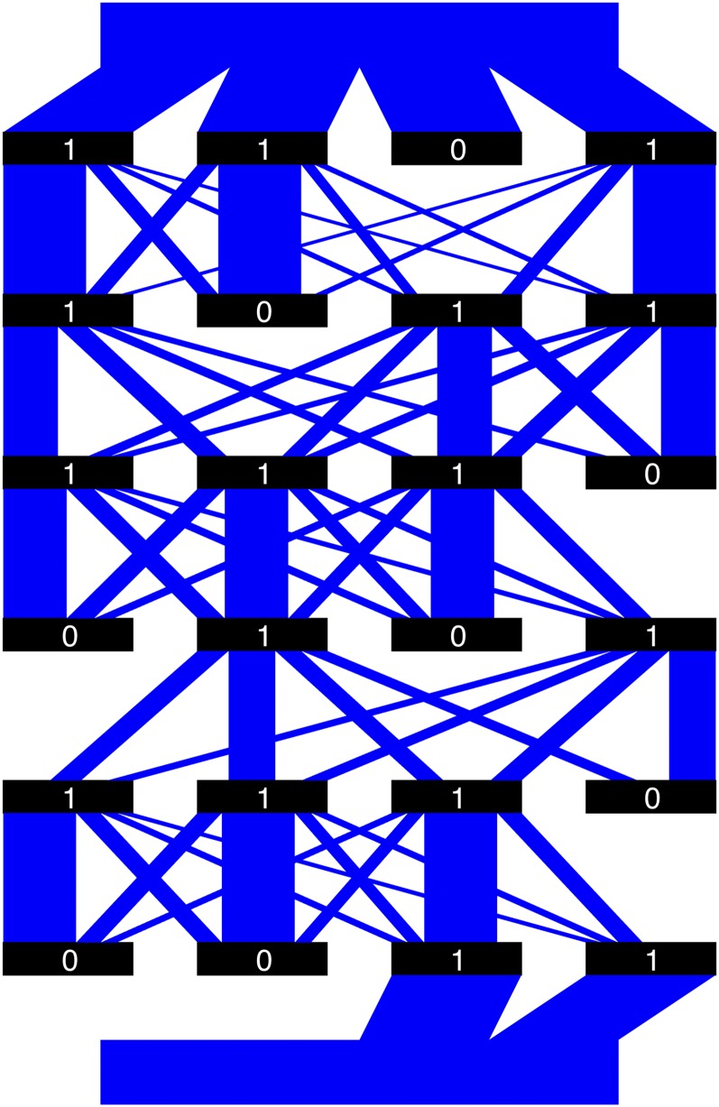
The plumbing system corresponding to Example 0.2 is illustrated in Figure 3, in which we removed those water pipes whose immediate upstream valves are closed. The transition matrix is $T_{:,:,1}=\left[\begin{array}{cccc}0.64& 0.16& 0.10& 0.10\\ 0.16& 0.64& 0.10& 0.10\\ 0.10& 0.10& 0.64& 0.16\\ 0.10& 0.10& 0.16& 0.64\end{array}\right],$ $T_{:,:,2}=\left[\begin{array}{cccc}0.4225& 0.2275& 0.1750& 0.1750\\ 0.2275& 0.4225& 0.1750& 0.1750\\ 0.1750& 0.1750& 0.4225& 0.2275\\ 0.1750& 0.1750& 0.2275& 0.4225\end{array}\right],$ $T_{:,:,3}=\left[\begin{array}{cccc}0.49& 0.21& 0.15& 0.15\\ 0.21& 0.49& 0.15& 0.15\\ 0.15& 0.15& 0.49& 0.21\\ 0.15& 0.15& 0.21& 0.49\end{array}\right],$ $T_{:,:,4}=\left[\begin{array}{cccc}0.36& 0.24& 0.20& 0.20\\ 0.24& 0.36& 0.20& 0.20\\ 0.20& 0.20& 0.36& 0.24\\ 0.20& 0.20& 0.24& 0.36\end{array}\right],$ $T_{:,:,5}=\left[\begin{array}{cccc}0.5625& 0.1875& 0.1250& 0.1250\\ 0.1875& 0.5625& 0.1250& 0.1250\\ 0.1250& 0.1250& 0.5625& 0.1875\\ 0.1250& 0.1250& 0.1875& 0.5625\end{array}\right],$ and the water matrix is $W=\left[\begin{array}{cccc}0.2500& 0.2500& 0& 0.2500\\ 0.2250& 0& 0.0900& 0.2100\\ 0.1476& 0.1037& 0.1252& 0\\ 0& 0.1006& 0& 0.0640\\ 0.0369& 0.0490& 0.0355& 0\\ 0& 0& 0.0307& 0.0174\end{array}\right].$ Therefore, the PCV is $0+0+0.0307+0.0174=\mathrm{0.0481.}$

Figure 3.

Illustration of the plumbing system for Example 0.2. Black rectangles are the valves, with binary numbers indicating whether they are open (1) or closed (0). The blue parallelograms are the water pipes, whose widths represent their relative volumes and not necessarily the actual amounts of water flowing through.

Conceptual distinctions of PCV, GEBV, and OHV

The fundamental difference between these three metrics is that GEBV and OHV assess the merit of two breeding parents as the summation of their separate breeding values, whereas PCV treats two breeding parents as a unique pair and selects the best pair that has the highest probability to produce an ideal gamete in two generations. We use the following simple example to demonstrate the conceptual distinctions of the three metrics.

Example 0.3. Consider 10 loci of interest in a population of 50 individuals. Rather than describing the genotypes of this population using a three-dimensional binary matrix defined in Mathematical formulation of the multi-allelic introgression process, we illustrate the information in Figure 4. A purple square is used to denote a “0” allele and a yellow square for a “1.” All the individuals in the sample of progeny are displayed abreast, so the figure contains a matrix of 10-by-100 purple-and-yellow squares. We will refer to the ith individual from the left as individual i. Then individuals 1, 2, 3, 5, and 18 can be represented, respectively, by

$$\left[\begin{array}{cc}0& 0\\ 1& 1\\ 1& 1\\ 1& 0\\ 1& 0\\ 1& 1\\ 1& 1\\ 1& 0\\ 0& 1\\ 1& 1\end{array}\right],\left[\begin{array}{cc}0& 0\\ 1& 1\\ 0& 1\\ 1& 1\\ 0& 1\\ 1& 1\\ 1& 0\\ 1& 1\\ 0& 1\\ 1& 1\end{array}\right],\left[\begin{array}{cc}0& 1\\ 1& 1\\ 0& 1\\ 1& 1\\ 0& 0\\ 1& 0\\ 0& 1\\ 1& 1\\ 1& 0\\ 1& 1\end{array}\right],\left[\begin{array}{cc}0& 0\\ 0& 1\\ 1& 1\\ 0& 1\\ 1& 0\\ 1& 0\\ 1& 0\\ 1& 1\\ 1& 0\\ 1& 1\end{array}\right],\text{and}\left[\begin{array}{cc}1& 1\\ 1& 0\\ 1& 0\\ 1& 1\\ 0& 1\\ 0& 1\\ 0& 1\\ 0& 1\\ 0& 0\\ 1& 0\end{array}\right].$$

The recombination-frequencies vector used in this example is

$$r={\left[\begin{array}{ccccccccc}0.1& 0.2& 0.1& 0.2& 0.1& 0.2& 0.1& 0.2& 0.1\end{array}\right]}^{\mathrm{\top }}.$$

The 50 individuals are ordered from left to right with a decreasing number of total desirable alleles, from 14 for individual 1 to 5 for individual 50.

Figure 4.

An illustration of 10 loci in a population consisting of 50 individuals. A purple square is used to denote a “0” allele and a yellow square for a “1.”

Solving Example 0.3 using the GEBV approach:

The GEBVs of the 50 individuals are calculated using Equation 3 and plotted in Figure 5.

Figure 5.

The GEBVs for Example 0.3.

The GEBV approach would select two individuals with the largest GEBVs, i.e., individuals 1 and 2, both with 14 desirable alleles. A limitation of this approach is that it compromises long-term potential for short-term gains. In this example, crossing individuals 1 and 2 will fix the first locus with undesirable alleles, eliminating the possibility of accumulating desirable alleles at this locus in subsequent generations.

Solving Example 0.3 using the OHV approach:

The OHV of the 50 individuals are calculated using Equation 4 and plotted in Figure 6.

Figure 6.

The OHVs for Example 0.3.

The OHV approach would select two individuals with the largest OHVs. Individual three has the largest OHV, whereas individuals 1, 2, 4, 5, 13, and 18 tie for the second place. A limitation of the OHV is the exclusive emphasis on the possibility without consideration of its probability. As such, the approach is unable to differentiate the six individuals with the same OHV based on their different likelihoods of combining nine desirable alleles into one gamete.

Solving Example 0.3 using the PCV approach:

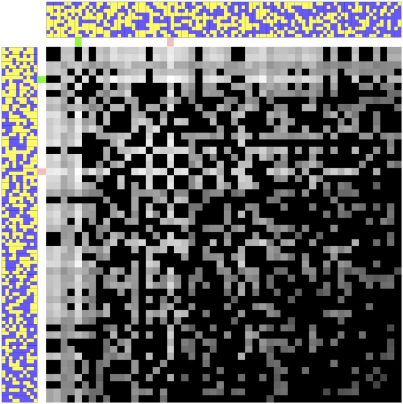
The PCVs of the 50 individuals are calculated using Equations 5 and 7–9 and plotted in Figure 7. The two subfigures at the top and left are the same population from Figure 4 with horizontal and vertical orientations, respectively. The largest subfigure is a PCV map. It consists of a 50-by-50 gray-shade matrix representing all PCV values for all possible pairs of breeding parents involving the 50 individuals in the population. As such, each square representing a PCV value has an area four times as large as the one that represents an allele in the horizontal and vertical subfigures. The brightness indicates the PCV for the two individuals directly above and to the left. The brighter the color in the PCV map, the higher the PCV. We point out four observations: (1) The PCV is not an additive function of two individuals. (2) The PCV map is symmetric across the diagonal, since the order of the two parents does not matter in the definition of PCV. (3) The diagonal represents PCVs for self-pollination. (4) The highest PCV is achieved by individuals 5 and 18, which are respectively highlighted in green and pink on the margins. These two individuals should be selected according to the PCV approach. Appendix B discusses two approaches that can be used to select the pair of individuals with the highest PCV from a population.

Figure 7.

The PCV map for Example 0.3. A purple square is used to denote a “0” allele and a yellow square for a “1.” The gray-shade matrix represents the PCVs of all possible pairs. The brighter the color, the larger the PCV. The two individuals with the largest PCV are highlighted in green and pink on the margins.

Compared with GEBV and OHV, PCV has two salient features. First, PCV evaluates each specific cross. In contrast, the GEBV and OHV calculate an estimated breeding value for each individual. In the context of mating designs, breeding values are analogous to general combining ability, whereas the PCV is analogous to specific combining ability. Second, the PCV integrates recombination frequencies to calculate conditional probabilities. In Example 0.3, out of the 1275 possible crosses, 711 have a zero PCV value because at least one locus will become homozygous for the undesirable allele. The remaining 564 combinations all have a unique PCV. Therefore, the PCV map in Figure 7 has 565 different shades of gray. In contrast, there are a large number of tied GEBVs and OHVs in the example.

Results

In this section, we describe and report results of simulated multi-allelic introgression experiments using the PCV, GEBV, and OHV approaches.

Experiment description:

We simulated a polygenic trait consisting of 100 QTL that are responsible for genetic variability in the trait. The locations of the QTL are distributed as uniform random variables among 10 simulated linkage groups. Each linkage group has from 8 to 12 QTL.

We considered two example trait-introgression projects. In both examples, the recipient and donor are homozygous at all QTL. In the first example, the recipient has desirable alleles at 93 of the QTL, while the donor has desirable alleles at the remaining 7. For reference, the recipient has undesirable alleles at C1Q4, C1Q6, C2Q9, C3Q1, C5Q4, C6Q3, and C6Q8, where CiQj denotes the jth QTL in chromosome i. In the second example, the recipient has desirable alleles at 80 of the loci, while the donor has desirable alleles at the remaining 20. For reference, the recipient has undesirable alleles at C1Q5, C1Q10, C2Q4, C2Q9, C3Q5, C3Q10, C4Q3, C4Q8, C5Q3, C5Q8, C6Q2, C6Q7, C6Q12, C7Q5, C7Q9, C8Q3, C8Q8, C9Q5, C9Q9, and C10Q3.

Recombination frequencies used in the simulation are given in Table 1. The value shown for column Ci and row Qj is the recombination frequency between the QTL pairs CiQj and $\mathrm{C}\left(i+1\right)\mathrm{Q}j.$ The value for the last QTL in a chromosome is 0.5, in accordance with the principle of independent assortment of chromosomes.

Table 1. The recombination frequencies used in the simulation.

	C1	C2	C3	C4	C5	C6	C7	C8	C9	C10
Q1	0.2725	0.2075	0.0569	0.0860	0.1414	0.0791	0.0126	0.2179	0.0659	0.0610
Q2	0.2649	0.1957	0.0759	0.1362	0.1693	0.1529	0.2951	0.1647	0.0102	0.0800
Q3	0.2148	0.0692	0.1452	0.1983	0.0285	0.3210	0.3044	0.2597	0.2480	0.2955
Q4	0.1262	0.1004	0.1037	0.0874	0.0875	0.1823	0.2654	0.2383	0.1667	0.0096
Q5	0.2705	0.1570	0.3078	0.2009	0.2670	0.1737	0.0329	0.3012	0.1600	0.1633
Q6	0.1776	0.0768	0.1434	0.2371	0.0097	0.0772	0.0873	0.2970	0.3016	0.0560
Q7	0.1169	0.2814	0.0616	0.0739	0.3096	0.1630	0.1118	0.1114	0.2033	0.3262
Q8	0.3130	0.0649	0.3016	0.0391	0.2434	0.2080	0.2266	0.5000	0.2059	0.5000
Q9	0.2920	0.5000	0.3266	0.0989	0.1629	0.2264	0.0455	—	0.2865	—
Q10	0.5000	—	0.1463	0.5000	0.5000	0.1318	0.2404	—	0.2685	—
Q11	—	—	0.5000	—	—	0.1225	0.5000	—	0.5000	—
Q12	—	—	—	—	—	0.5000	—	—	—	—

We implemented the breed function to simulate the introgression project, with the simulated genomes as the initial population for each example. In subsequent generations, 100 progeny were sampled from simulated crosses of two individuals selected from the previous generation. The recipient line is treated as a member of the sample so that backcrossing is always an option. Four versions of the select function were compared:

1. The GEBV approach, which selects two different individuals with the highest GEBVs.

2. The OHV approach, which selects two different individuals with the highest OHVs.

3. The PCV-I approach, which selects two different individuals with the highest PCV.

4. The PCV-II approach, which selects one (for self-pollination) or two (for cross-pollination) individuals with the highest PCV.

A total of 1000 simulation runs were carried out, and the comparison was based on the time and probability of success, i.e., number of generations to completely introgress all desirable donor alleles. The simulation was implemented and results were generated using GNU Octave (Eaton et al. 2015).

Results for Example 1:

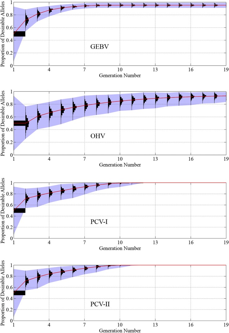
Figure 8 plots the population histograms of the proportion of desirable alleles in the genome over time. For all selection approaches, the sample representing the first generation consists of the recipient line (with 93% of the desirable alleles), the donor line (with 7% of the desirable alleles), and 98 F₁ lines consisting of half of the alleles from the recipient and donor (with 50% of the desirable alleles). The histogram for progeny in generation two is the same for GEBV, PCV-I, and PCV-II because the recipient parent was crossed to the F₁ for these selection approaches. On the other hand, the histogram for the OHV approach is represented by a doubled-haploid sample from the F₁. When GEBV and OHV are used, the average proportions of desirable alleles reach 95 and 93% in the 19th generation, respectively. When PCV-I and PCV-II are used, an ideal progeny will be produced in as early as 7 generations and no later than the 11th.

Figure 8.

Performance of the GEBV, OHV, PCV-I, and PCV-II approaches in 1000 simulation runs of trait introgression of seven QTL. The vertical axis represents the proportion of desirable alleles in the genome. Histograms of the proportion of desirable alleles among 100 progeny from 1000 simulation runs are plotted for each generation. The red curve shows the population mean.

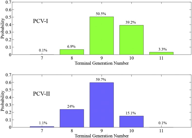
Figure 9 compares the probability distributions of the terminal generation for PCV-I and PCV-II approaches. On average, the PCV-I approach takes 9.4 generations to produce an ideal progeny, whereas PCV-II takes 8.9 generations. Thus, allowing self-pollination during the breeding process increased the efficiency of the project by half a generation in this example.

Figure 9.

Distributions of the terminal generation numbers of PCV-I and PCV-II approaches.

Result for Experiment 2:

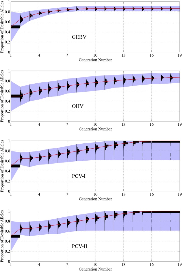
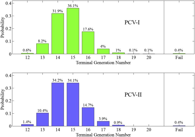
Figure 10 and Figure 11 reveal similar results of the four selection approaches as Figure 8 and Figure 9, but, as expected, all approaches take more generations to plateau. Using the GEBV and OHV approaches, the proportions of desirable alleles reach 86 and 90% in the 19th generation, respectively. Out of the 1000 simulation repetitions, both PCV-I and PCV-II approaches successfully produced an ideal progeny 996 times, taking an average of 14.8 and 14.7 generations, respectively. In the other four times, the trait introgression project failed by having at least one locus become homozygous with undesirable alleles for all individuals in the population. The GEBV and OHV approaches failed in the same way in all 1000 simulation runs in both experiments.

Figure 10.

Performance of the GEBV, OHV, PCV-I, and PCV-II approaches in 1000 simulation runs of trait introgression of 20 QTL.

Figure 11.

Distributions of the terminal generation numbers of PCV-I and PCV-II approaches.

Data availability

The authors state that all data necessary for confirming the conclusions presented in the article are represented fully within the article. The electronic version of the data files in Octave format can be downloaded from https://sites.google.com/view/lizhiwang.

Discussion

With a few exceptions (Johnson et al. 1988; Canzar and El-Kebir 2011; Xu et al. 2011; De Beukelaer et al. 2015; Akdemir and Sanchez 2016), genetic improvement projects in crop species have not been approached using the tools of operations research. On the other hand, the optimization challenge of maximizing genetic gain while minimizing inbreeding in animal breeding has been approached extensively using linear programming, genetic algorithms, integer programming, and semidefinite programming (Woolliams et al. 2015). We formulated the multi-allelic introgression challenge as a mathematical process and we hope that it will attract other operations researchers, applied mathematicians, and computational scientists to contribute to genetic improvement projects.

We framed the challenge of introgressing multiple alleles from a homozygous donor to a homozygous recipient using time (number of generations) and proportions of desirable alleles in each generation of progeny as quantitatively measurable criteria for comparing breeding strategies. Missing from these criteria is a consideration of cost. In general, the number of progeny evaluated every generation can serve as a surrogate for cost, and in future research we will look at the relative impacts of sample size for each generation of evaluation. While these costs are relatively easy to quantify, considerable thought will be needed to formulate either social or commercial costs associated with slower introgression of alleles of economically important traits.

The PCV is a new metric for selection of parents. Rather than sticking to predetermined breeding strategies such as backcrossing, as widely used for trait introgression, PCV-based selection identifies the pair of individuals whose complementary genotypes have the highest probability to yield an ideal gamete in two generations. The simulation results demonstrated that the PCV outperforms the existing GEBV and OHV approaches.

Meaningful future work would be to conduct a comprehensive comparison with more recently invented selection approaches that appear to be very promising. For example, Woolliams et al. (2015) proposed the optimal contribution selection, which attempts to maximize genetic gain in the next generation. Akdemir and Sanchez (2016) propose genomic mating as an alternative to genomic selection, which “uses concepts of estimated breeding values, risk (usefulness) and coefficient of ancestry to optimize mating between parents.” They also discussed alternative risk measures that include LD information.

Applicability of our approach is limited by a number of simplifying assumptions summarized in Simplifying assumptions. Relaxing these will provide potentially fruitful topics for future research. For example, a similar, but more sophisticated, definition of the PCV could be designed for autopolyploid perennial crops such as alfalfa. Also, if desirable alleles of interest are carried by multiple donors, then modifications are required to extend the PCV. Two approaches have been proposed for introgression of multiple alleles from multiple donors. One is to sequentially introgress alleles from each donor, and the other is to stack all their desirable alleles into a single donor line (Peng et al. 2014a,b). A couple of optimization approaches have been proposed for the gene-stacking problem (Canzar and El-Kebir 2011; Xu et al. 2011), which has been proved to be nondeterministic polynomial-time hard (Xu et al. 2011). It would be a challenging but useful extension to design PCV-based breeding strategies for multiple donors. The selection of less than one pair of parent lines must be coordinated to not only produce enough seeds to allow for critical recombinations to occur, but also to expedite the integration of all desirable alleles into the recipient cultivar(s).

The selection approach demonstrated in Simulation experiments applies to species that can produce a large number of progeny from a cross (such as corn, sunflower, and sorghum). Two strategies can be used to apply this approach to less productive species (such as soybean, wheat, and peanut). One is to compensate the small progeny size with a large number of crosses by selecting multiple pairs of parents using the PCV metric repeatedly. The other is to extend the PCV definition to select multiple pairs of parents and explicitly include the numbers of crosses and expected progeny as parameters, which is one of our future research topics.

Another direction that deserves investigation in future research is the exploration of more optimal breeding strategies. The trait-introgression breeding problem formulated in the Formulation section, even with the simplifying assumptions, is too complex to be readily solvable by existing optimization methodology. Although the PCV-based multi-allelic introgression outperforms those based on breeding values, it is unclear to us how much further improvement could be made. A starting point could be to dynamically adjust the number of individuals evaluated every generation and the selection approach in each generation in response to the outcome of the previous cross.

Appendix A: Lemmas and Proofs

The following lemma is a straightforward derivation from the definitions in the Multi-allelic introgression as an algorithmic process section.

Lemma 0.1. For all $i\in \left\{1,\dots ,N\right\},$ we have:

$$g_i=\{\begin{array}{ll}{L}_{i,1}\hfill & \text{if }{J}_i^1=0\text{ and }{J}_i^3=0;\hfill \\ L_{i,2}\hfill & \text{if }{J}_i^1=1\text{ and }{J}_i^3=0;\hfill \\ L_{i,3}\hfill & \text{if }{J}_i^2=0\text{ and }{J}_i^3=1;\hfill \\ L_{i,4}\hfill & \text{if }{J}_i^2=1\text{ and }{J}_i^3=1.\hfill \end{array}$$ (A1)

The following lemma reveals the rationale behind the definition for the transition matrix.

Lemma 0.2. For all $i\in \left\{1,\dots ,N-1\right\},$$j\in \left\{1,2,3,4\right\},$ and $k\in \left\{1,2,3,4\right\},$ we have

$$P\left(g_{i+1}=L_{i+1,j}|g_i=L_{i,k}\right)=T_{k,j,i}.$$

Proof. For all $i\in \left\{1,\dots ,N-1\right\},$ we prove the equation for $j=1$ and $k\in \left\{1,2,3\right\}.$ The proof for the other cases is similar:

$$\begin{array}{c}P\left(g_{i+1}=L_{i+1,1}|g_i=L_{i,1}\right)\\ =P\left(J_{i+1}^1=0,J_{i+1}^3=0|J_i^1=0,J_i^3=0\right)\\ =P\left(J_{i+1}^1=0|J_i^1=0,J_i^3=0\right)P\left(J_{i+1}^3=0|J_i^1=0,J_i^3=0\right)\\ =P\left(J_{i+1}^1=0|J_i^1=0\right)P\left(J_{i+1}^3=0|J_i^3=0\right)\\ ={\left(1-r_i\right)}^2\\ =T_{1,1,i}.\end{array}$$

$$\begin{array}{c}P\left(g_{i+1}=L_{i+1,2}|g_i=L_{i,1}\right)\\ =P\left(J_{i+1}^1=1,J_{i+1}^3=0|J_i^1=0,J_i^3=0\right)\\ =P\left(J_{i+1}^1=1|J_i^1=0,J_i^3=0\right)P\left(J_{i+1}^3=0|J_i^1=0,J_i^3=0\right)\\ =P\left(J_{i+1}^1=1|J_i^1=0\right)P\left(J_{i+1}^3=0|J_i^3=0\right)\\ =r_i\left(1-r_i\right)\\ =T_{1,2,i}.\end{array}$$

$$\begin{array}{l}P\left(g_{i+1}=L_{i+1,3}|g_i=L_{i,1}\right)\\ =P\left(J_{i+1}^2=1,J_{i+1}^3=0|J_i^1=0,J_i^3=0\right)\\ =P\left(J_{i+1}^2=1|J_i^1=0,J_i^3=0\right)P\left(J_{i+1}^3=0|J_i^1=0,J_i^3=0\right)\\ =P\left(J_{i+1}^2=1\right)P\left(J_{i+1}^3=1|J_i^3=0\right)\\ =0.5r_i\\ =T_{1,3,i}.\end{array}$$

Proof for Proposition 0.1:

Proof. We establish the respective equivalence between Equation 6 and Equations 7 and 8 as follows.

Equation 6 for $i=1$ and Equation 7 are equivalent because for all $j\in \left\{1,2\right\},$ we have

$$\begin{array}{c}{W}_{1,j}=P\left(g_1=1,g_1=L_{1,j}^1\right)\\ =P\left(L_{1,j}^1=1,g_1=L_{1,j}^1\right)\\ =L_{1,j}^{1}P\left(g_1=L_{1,j}^1\right)\\ =L_{1,j}^{1}P\left(J_1^1=j-1,J_1^3=0\right)\\ =L_{1,j}^{1}P\left(J_1^1=j-1\right)P\left(J_1^3=0\right)\\ =\frac{1}{4}{L}_{1,j}^1.\end{array}$$

The case for $j\in \left\{3,4\right\}$ is similar.

Equation 6 for $i\in \left\{2,\dots ,N\right\}$ and Equation 8 are equivalent because for all $i\in \left\{2,\dots ,N\right\}$ and $j\in \left\{1,2,3,4\right\},$ we have

$$\begin{array}{c}{W}_{i,j}=P\left(g_1=\dots =g_i=1,g_i=L_{i,j}\right)\\ =P\left(g_1=\dots =g_{i-1}=1,g_i=L_{i,j},L_{i,j}=1\right)\\ =L_{i,j}P\left(g_1=\dots =g_{i-1}=1,g_i=L_{i,j}\right)\\ =L_{i,j}{\displaystyle \sum _{k=1}^{4}P\left(g_1=\dots =g_{i-1}=1,g_{i-1}=L_{i-1,k},g_i=L_{i,j}\right)}\\ =L_{i,j}{\displaystyle \sum _{k=1}^{4}P\left(g_i=L_{i,j}|g_1=\dots =g_{i-1}=1,g_{i-1}=L_{i-1,k}\right)}\\ \times P\left(g_1=\dots =g_{i-1}=1,g_{i-1}=L_{i-1,k}\right)\\ =L_{i,j}{\displaystyle \sum _{k=1}^{4}P\left(g_i=L_{i,j}|g_{i-1}=L_{i-1,k}\right)W_{i-1,k}}\\ =L_{i,j}{\displaystyle \sum _{k=1}^4{T}_{k,j,i-1}{W}_{i-1,k}}.\end{array}$$

Proof for Proposition 0.2:

Proof.

$$\begin{array}{c}\text{PCV}\left(L^1,L^2,r\right)=P\left(g_1=\dots =g_N=1\right)\\ ={\displaystyle \sum _{j=1}^{4}P\left(g_1=\dots =g_N=1,g_N=L_{N,j}\right)}\\ ={\displaystyle \sum _{j=1}^4{W}_{N,j}}.\end{array}$$

Appendix B: Optimization of PCV

We present an optimization model that can be used to select the optimal pair of individuals with the highest PCV from a given population.

The model takes two parameters as input: the set of progeny of lines $P\in {\mathbb{B}}^{N\times 2\times K},$ with K being the number of lines and the recombination frequencies vector $r\in {\left[0,0.5\right]}^{N-1}.$ There are three sets of decision variables:

1. $t\in {\mathbb{B}}^{2\times K}$ is a binary variable, indicating whether $\left(t_{m,k}=1\right)$ or not $\left(t_{m,k}=0\right)$ line k is selected as the mth parent, for all $m\in \left\{1,2\right\}$ and $k\in \left\{1,\dots ,K\right\}.$

2. $x\in {\mathbb{B}}^{N\times 4}$ represents the genotypes of the two selected parents. If $t_{1,k^1}=t_{2,k^2}=1,$ then $x_{:,1:2}=P_{:,:,k^1}$ and $x_{:,3:4}=P_{:,:,k^2}.$

3. $w\in {\mathbb{B}}^{N\times 4}$ is the water matrix of x.

The optimization model is presented in (B2)–(B9), which is a mixed integer linear program (MILP). The objective function (B2) calculates the PCV of the two selected parent lines, which is to be maximized. Constraint (B3) requires that exactly two breeding parents are selected from the population, which could possibly be the same line. Constraints (B4) and (B5) assign the genotypes of the selected lines from the breeding population to the x matrix. Constraints (B6)–(B8) calculate the water matrix for x. Constraint (B6) is equivalent to Equation 7, and the two linear inequalities (B7) and (B8) are equivalent to

$$w_{i,j}\le x_{i,j}{\displaystyle \sum _{k=1}^4{T}_{k,j,i-1}{w}_{i-1,j}}.$$ (B1)

Due to the objective function, inequality (B1) will hold at equality when the model (B2)–(B9) is solved to optimality, which is equivalent to Equation 8. Constraint (B9) defines the types and ranges of the decision variables. This MILP model can be solved to optimality by existing algorithms and software.

$$\underset{w,x,t}{\max }{\displaystyle \sum _{k=1}^4{w}_{N,k}}$$ (B2)

$$\text{subject}\hspace{0.17em}\text{to}\hspace{1em}{\displaystyle \sum _{k=1}^K{t}_{m,k}}=1\forall m=1,2$$ (B3)

$$x_{i,j}={\displaystyle \sum _{k=1}^K{t}_{1,k}{P}_{i,j,k}}\forall i\in \left\{1,\dots ,N\right\};\forall j\in \left\{1,2\right\}$$ (B4)

$$x_{i,j}={\displaystyle \sum _{k=1}^K{t}_{2,k}{P}_{i,j-2,k}}\forall i\in \left\{1,\dots ,N\right\};\forall j\in \left\{3,4\right\}$$ (B5)

$$w_{1,j}=0.25x_{1,j}\forall j\in \left\{1,2,3,4\right\}$$ (B6)

$$w_{i,j}\le x_{i,j}\forall i\in \left\{2,\dots ,N\right\},\forall j\in \left\{1,2,3,4\right\}$$ (B7)

$$w_{i,j}\le \stackrel{4}{{\displaystyle \sum }_{k=1}}{T}_{k,j,i-1}{w}_{i-1,j},\forall i\in \left\{2,\dots ,N\right\},\forall j\in \left\{1,2,3,4\right\}$$ (B8)

$$0\le w\le 1;x,t\text{ binary}.$$ (B9)

Alternatively, the optimal selection of breeding parents can be achieved via a brute-force enumeration of all possible $\frac{1}{2}n\left(n+1\right)$ combinations (excluding symmetric duplications).

Literature Cited

- Akdemir D., Sanchez J., 2016. Efficient breeding by genomic mating. Front. Genet. 7: 210. [DOI] [PMC free article] [PubMed] [Google Scholar]
- Bernardo R., 2009. Genomewide selection for rapid introgression of exotic germplasm in maize. Crop Sci. 49: 419–425. [Google Scholar]
- Bonk S., Reichelt M., Teuscher F., Segelke D., Reinsch N., 2016. Mendelian sampling covariability of marker effects and genetic values. Genet. Sel. Evol. 48: 36. [DOI] [PMC free article] [PubMed] [Google Scholar]
- Canzar, S., and M. El-Kebir, 2011 A Mathematical Programming Approach to Marker-Assisted Gene Pyramiding, pp. 26–38 in Algorithms in Bioinformatics (Lecture notes in Computer Science, Vol. 6833), edited by T. M. Przytycka and M.-F. Sagot. Springer-Verlag, Berlin. [Google Scholar]
- Cavanagh C. R., Chao S., Wang S., Huang B. E., Stephen S., et al. , 2013. Genome-wide comparative diversity uncovers multiple targets of selection for improvement in hexaploid wheat landraces and cultivars. Proc. Natl. Acad. Sci. USA 110: 8057–8062. [DOI] [PMC free article] [PubMed] [Google Scholar]
- Daetwyler H. D., Hayden M. J., Spangenberg G. C., Hayes B. J., 2015. Selection on optimal haploid value increases genetic gain and preserves more genetic diversity relative to genomic selection. Genetics 200: 1341–1348. [DOI] [PMC free article] [PubMed] [Google Scholar]
- De Beukelaer H., De Meyer G., Fack V., 2015. Heuristic exploitation of genetic structure in marker-assisted gene pyramiding problems. BMC Genet. 16: 2. [DOI] [PMC free article] [PubMed] [Google Scholar]
- Eaton J. W., Bateman D., Hauberg S., Wehbring R., 2015. GNU Octave version 4.0.0 manual: a high-level interactive language for numerical computations.
- Frisch M., Melchinger A. E., 2005. Selection theory for marker-assisted backcrossing. Genetics 170: 909–917. [DOI] [PMC free article] [PubMed] [Google Scholar]
- Frisch M., Bohn M., Melchinger A. E., 1999. Comparison of selection strategies for marker-assisted backcrossing of a gene. Crop Sci. 39: 1295–1301. [Google Scholar]
- Gorjanc G., Jenko J., Hearne S. J., Hickey J. M., 2016. Initiating maize pre-breeding programs using genomic selection to harness polygenic variation from landrace populations. BMC Genomics 17: 30. [DOI] [PMC free article] [PubMed] [Google Scholar]
- Haldane J., 1919. The combination of linkage values and the calculation of distances between the loci of linked factors. J. Genet. 8: 299–309. [Google Scholar]
- Johnson B., Dauer J., Gardner C., 1988. A model for determining weights of traits in simultaneous multitrait selection. Appl. Math. Model. 12: 556–564. [Google Scholar]
- Kumar G. R., Sakthivel K., Sundaram R. M., Neeraja C. N., Balachandran S., et al. , 2010. Allele mining in crops: prospects and potentials. Biotechnol. Adv. 28: 451–461. [DOI] [PubMed] [Google Scholar]
- Leung H., Raghavan C., Zhou B., Oliva R., Choi I. R., et al. , 2015. Allele mining and enhanced genetic recombination for rice breeding. Rice (N. Y.) 8: 34. [DOI] [PMC free article] [PubMed] [Google Scholar]
- Longin C. F. H., Reif J. C., 2014. Redesigning the exploitation of wheat genetic resources. Trends Plant Sci. 19: 631–636. [DOI] [PubMed] [Google Scholar]
- McCouch S. R., McNally K. L., Wang W., Hamilton R. S., 2012. Genomics of gene banks: a case study in rice. Am. J. Bot. 99: 407–423. [DOI] [PubMed] [Google Scholar]
- Meuwissen T., Hayes B., Goddard M., 2001. Prediction of total genetic value using genome-wide dense marker maps. Genetics 157: 1819–1829. [DOI] [PMC free article] [PubMed] [Google Scholar]
- Peng T., Sun X., Mumm R. H., 2014a Optimized breeding strategies for multiple trait integration: I. Minimizing linkage drag in single event introgression. Mol. Breed. 33: 89–104. [DOI] [PMC free article] [PubMed] [Google Scholar]
- Peng T., Sun X., Mumm R. H., 2014b Optimized breeding strategies for multiple trait integration: II. Process efficiency in event pyramiding and trait fixation. Mol. Breed. 33: 105–115. [DOI] [PMC free article] [PubMed] [Google Scholar]
- Servin B., Martin O. C., Mézard M., Hospital F., 2004. Toward a theory of marker-assisted gene pyramiding. Genetics 168: 513–523. [DOI] [PMC free article] [PubMed] [Google Scholar]
- van Berloo R., Stam P., 1998. Marker-assisted selection in autogamous ril populations: a simulation study. Theor. Appl. Genet. 96: 147–154. [Google Scholar]
- Visscher P. M., Haley C. S., Thompson R., 1996. Marker-assisted introgression in backcross breeding programs. Genetics 144: 1923–1932. [DOI] [PMC free article] [PubMed] [Google Scholar]
- Woolliams J., Berg P., Dagnachew B., Meuwissen T., 2015. Genetic contributions and their optimization. J. Anim. Breed. Genet. 132: 89–99. [DOI] [PubMed] [Google Scholar]
- Xu P., Wang L., Beavis W. D., 2011. An optimization approach to gene stacking. Eur. J. Oper. Res. 214: 168–178. [Google Scholar]
Associated Data
This section collects any data citations, data availability statements, or supplementary materials included in this article.
Data Availability Statement