Instrumental Variable Analyses and Selection Bias

Abstract

Instrumental variables (IV) are used to draw causal conclusions about the effect of exposure E on outcome Y in the presence of unmeasured confounders. IV assumptions have been well described: 1) IV affects E; 2) IV affects Y only through E; 3) IV shares no common cause with Y. Even when these assumptions are met, biased effect estimates can result if selection bias allows a non-causal path from E to Y. We demonstrate the presence of bias in IV analyses on a sample from a simulated dataset, where selection into the sample was a collider on a non-causal path from E to Y. By applying inverse probability of selection weights we were able to eliminate the selection bias. IV approaches may protect against unmeasured confounding but are not immune from selection bias. Inverse probability of selection weights used with IV approaches can minimize bias.

Background

Instrumental variables (IV) are used to draw causal conclusions about the effect of exposure E on outcome Y in the presence of unmeasured confounders. Details of IV analyses have been described in detail elsewhere^1–4. Briefly, for a variable to be an IV, three assumptions must be met: 1) IV affects E, 2) IV affects the Y only through E, and 3) IV does not share a common cause with Y^3–5.

Several challenges to a successful IV analysis have been well documented, most of which focus on the consequences of choosing an inadequate instrument or violating one of the three key assumptions^5–7. For example, a weak association between the instrument and exposure can lead to biased results or large standard error⁶. Additionally, IV analyses are unable to address the problem of confounding by indication since the strong relationship of the confounder on exposure limits the strength of the effect of the IV on exposure ^6,8,9.

These challenges represent important limitations to IV analyses and must be carefully considered. However, we contend that satisfying the key assumptions and avoiding challenges associated with instrument selection is insufficient to guarantee an unbiased result. Even when these assumptions are met, conditioning on selection (e.g., as in a complete cohort analysis) can bias results if selection is a collider on a non-causal path from E to Y. The focus of this paper is to illustrate the impact of selection bias in IV analyses and to demonstrate the use of inverse probability of selection weights to mitigate bias due to selection.

Methods

We conducted a simulation to estimate the association between outcome Y and exposure E under multiple scenarios: 1) confounded, 2) confounder-adjusted, 3) confounded and subject to selection bias, 4) confounder-adjusted and subject to selection bias, 5) confounded and corrected for selection bias, 6) fully adjusted.

We simulated 1000 datasets each with 5000 observations of 6 variables. We created an unmeasured confounder U and measured variable C, each distributed Normal (0,1). We generated IV as a Bernoulli random variable with probability 0.4. The primary exposure of interest, E, was assigned a Bernoulli random variable with probability expit(log(0.25)+log(3.0)IV+log(1.7)U) where expit(·)=exp(·)/[exp(·)+1]. The outcome, Y, was drawn from a normal distribution with mean 5+1.5U+2.0E+1.4C and variance 1. Finally, we generated a binary indicator S with probability expit(log(0.67)+log(2.2)C+log(5.0)E), such that restricting to observations with S=1 would open a non-causal pathway from E→[S]←C→Y. Overall, the probability of S=1 was 51%. Figure 1 depicts the relationship between all variables in a directed acyclic graph (DAG).

Figure 1.

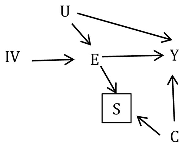
Directed Acyclic Graph (DAG) depicting the association between exposure E and outcome Y with unmeasured confounder U. Selecting on binary selection variable, S, induces a non-causal pathway between the instrumental variable (IV) and Y through E→[S]←C→Y.

Within each simulated dataset, we estimated the crude effect of E on Y using a linear regression model (Model 1). Then, following traditional IV methodology, we fit a two-stage least squares regression to estimate the average effect of E on Y unconfounded by measured and unmeasured covariates (Model 2). The two-stage least squares regression first models the treatment as a function of the instrument, and then models the outcome given the predicted treatment^1,4,10. For simplicity, we simulated data in which the effect of the treatment is constant. Under this homogeneity assumption, the IV method estimates the average causal effect in the population. Though the simulated nature of our data guaranteed that we satisfied the criteria of an IV analysis, investigators applying this methodology should be aware that the IV conditions are not guaranteed to hold in practice¹¹.

We also ran the linear model for the (confounded) effect of E on Y and the two-stage least squares model within the subset of the data with S=1 (Models 3 and 4) to demonstrate the impact of selection bias. Finally, we applied inverse probability of selection weights to the selected-sample linear and two-stage least squares models to correct for the induced selection bias, both with and without confounding (Models 5 and 6). Individuals with S=1 were given weights that were the inverse of the probability of S=1 in the entire sample, conditional on covariates. The denominator of the weights were estimated based on predicted probabilities from a logistic regression model for S based on E and C¹². To obtain an estimate for the variance of the inverse probability of selection-weighted models, we resampled the from each simulated dataset 200 times, estimated the weights within each sample, and fit the weighted models within each sample. The standard deviation of the 200 estimates was taken as an estimate of the standard error for the point estimate; we used it to create 95% confidence intervals using the Wald formula¹³.

We calculated percent bias as the difference between the true and estimated effect of E on Y divided by the true effect. Coverage probabilities were estimated based on the proportion of 95% confidence intervals across the 1000 samples that captured the true estimate. We report the median percent bias, mean squared error (MSE) and 95% coverage probability for the effect of E on Y in each scenario.

R code for the simulation is presented in the eAppendix.

Results

In the full sample, the median point estimate indicated that persons with E=1 had a value of Y that was 2.7 units higher than persons with E=0 using the crude (confounded) linear regression model. The median percent bias compared to the truth (β=2.0) was 36% [interquartile range (IQR): 33%, 38%], with an MSE of 0.51 and 95% coverage probability of 0%. The median point estimate using the two-stage least squares model in the full sample was 2.0, indicating −1% bias (IQR: −11%, 10%), an MSE of 0.10 and 95% coverage probability of 94%.

After restricting analyses to the subset of observations with S=1, the crude linear regression model resulted in a median point estimate of 2.4 and median percent bias of 20% (IQR: 17%, 23%), with MSE of 0.17 and 95% coverage probability of 1%. Using a two-stage least squares model in the observations where S=1, the median percent bias decreased to −11% (IQR: −23, 2%) with an MSE of 0.18 and 95% coverage probability of 90%. The inverse probability of selection-weighted linear model produced a median point estimate of 2.7, with 36% median percent bias (IQR: 32%, 39%), an MSE of 0.52, and 95% coverage probability of 0%. Weighting the two-stage least squares model by the inverse probability of selection weights reduced the bias to 1% (IQR: −17, 19%) with an MSE of 0.27 and 95% coverage probability of 96% (Table 1).

Table 1.

Median point estimates, percent bias, and 95% coverage intervals for the effect of exposure E on outcome Y in the full and selected simulated samples

	Full Sample		Selected Sample
	Model 1: Unadjusted linear regression	Model 2: Two-stage least squares	Model 3: Unadjusted linear regression	Model 4: Two-stage least squares	Model 5: Weighted linear regression	Model 6: Weighted two-stage least squares
Median point estimate (IQR)	2.7 (2.7, 2.8)	2.0 (1.8, 2.2)	2.4 (2.3, 2.5)	1.8 (1.6, 2.0)	2.7 (2.7, 2.8)	2.0 (1.7, 2.4)
Median variance (IQR)	0.07 (0.07, 0.07)	0.30 (0.29, 0.31)	0.09 (0.09, 0.09)	0.36 (0.34, 0.38)	0.10 (0.09, 0.10)	0.52 (0.47, 0.57)
Median percent bias (IQR)	36 (33, 38)	−1.1 (−11, 10)	20 (17, 23)	−11 (−23, 1.5)	36 (32, 39)	1.3 (−17, 19)
Mean squared error	0.51	0.10	0.17	0.18	0.52	0.27
95% coverage interval	0%	94%	1%	90%	0%	96%

IQR indicates interquartile range.

Discussion

In our simulation, we demonstrated the presence of confounding and the use of IV analysis to control that confounding. The two-stage least squares regression model correctly accounted for confounding in the full sample, reiterating the benefit of a two-stage least squares model when an appropriate instrument is chosen^2,4,7. However, despite fulfilling the commonly cited criteria for IV (IV affects E; IV affects the Y only through E; and IV does not share a common cause with Y), the two-stage least squares model showed large bias in the unweighted, selected sample. This simulation highlights that while IV analyses can account for unmeasured confounding, they are still subject to selection bias.

In comparative effectiveness studies, selection can bias IV analyses when the analysis is restricted to participants receiving a subset of all treatment options^14,15. Similarly, IV analyses are subject to selection bias when selection into the analytic sample from the source population is a collider¹⁶. The resulting selection bias is a violation of exchangeability, which is conceptually equivalent to a violation of the third IV assumption¹⁴. Following the rules for causal DAGs³, by conditioning (through restriction) on S, a collider, the parent nodes of S are correlated (Figure 1), thus creating a non-causal pathway from E to Y¹⁶. Therefore, there is a non-causal path from IV to Y suggesting that IV analyses should be biased^17,18. We confirmed and illustrated the presence of this bias with our simple simulation. Our simulation used two-stage least squares models, but we expect to see similar results using any IV method that does not explicitly block the non-causal pathway from E to Y. Additionally, although the IV was causal in our simulation, we would expect to see a similar bias due to selection when the instrument is non-causal as well.

To correct for bias caused by selection, IPSW create a pseudo-population that is representative of the study sample in the absence of selection^12,19. This commonly recommended method to address selection bias proved useful in reducing bias in our simulated IV analysis with the selected sample. In the simulation, we created inverse probability of selection weights based on the exposure and measured variable C. Such weights can be easily applied to any traditional two-stage least squares regression model to minimize selection bias.

It should be noted that while inverse probability of selection weights estimators may reduce bias (under a set of assumptions), they typically have higher variance than unweighted estimators, resulting in a larger MSE. The magnitude of the MSE in IV analyses depends in part on the strength of the IV-E relationship, whereby a stronger relationship results in a lower MSE¹⁴.

Investigators pursing an IV approach must understand how their analytical sample is derived to assess the threat of selection bias. IV approaches may protect against unmeasured confounding but do not solve problems of selection bias. Inverse probability of selection weights may be used in a two-stage least squares model to minimize the threat of bias from both unmeasured confounding and selection bias.

References

- 1.Ginsberg W. Instrumental Variables: Some Generalizations. Am Stat. 1971;25(2):25. doi: 10.2307/2682003. [DOI] [Google Scholar]
- 2.Newhouse JP, McClellan M. Econometrics in outcomes research: the use of instrumental variables. Annu Rev Public Heal. 1998;19:17–34. doi: 10.1146/annurev.publhealth.19.1.17. [DOI] [PubMed] [Google Scholar]
- 3.Greenland S. An introduction to instrumental variables for epidemiologists. Int J Epidemiol. 2000;29:722–729. doi: 10.1093/ije/29.4.722. [DOI] [PubMed] [Google Scholar]
- 4.Angrist JD, Imbens GW, Rubin DB. Identification of Causal Effects Using Instrumental Variables. J Am Stat Assoc. 1996;91:444–455. doi: 10.2307/2291629. [DOI] [Google Scholar]
- 5.Hernán MA, Robins JM. Instruments for causal inference: an epidemiologist’s dream? Epidemiology. 2006;17(4):360–372. doi: 10.1097/01.ede.0000222409.00878.37. [DOI] [PubMed] [Google Scholar]
- 6.Martens EP, Pestman WR, de Boer A, Belitser SV, Klungel OH. Instrumental variables: application and limitations. Epidemiology. 2006;17(3):260–267. doi: 10.1097/01.ede.0000215160.88317.cb. [DOI] [PubMed] [Google Scholar]
- 7.Hogan JW, Lancaster T. Instrumental variables and inverse probability weighting for causal inference from longitudinal observational studies. Stat Methods Med Res. 2004;13(1):17–48. doi: 10.1191/0962280204sm351ra. [DOI] [PubMed] [Google Scholar]
- 8.Bosco JLF, Silliman RA, Thwin SS, et al. A most stubborn bias: no adjustment method fully resolves confounding by indication in observational studies. J Clin Epidemiol. 2010;63:64–74. doi: 10.1016/j.jclinepi.2009.03.001. [DOI] [PMC free article] [PubMed] [Google Scholar]
- 9.Fang G, Brooks JM, Chrischilles EA. Comparison of instrumental variable analysis using a new instrument with risk adjustment methods to reduce confounding by indication. Am J Epidemiol. 2012;175:1142–1151. doi: 10.1093/aje/kwr448. [DOI] [PubMed] [Google Scholar]
- 10.Angrist JD, Imbens GW. Two-Stage Least Squares Estimation of Average Causal Effects in Models with Variable Treatment Intensity. J Am Stat Assoc. 1995;90(430):431–442. doi: 10.1080/01621459.1995.10476535. [DOI] [Google Scholar]
- 11.Swanson SA, Hernán MA. How to Report Instrumental Variable Analyses (Suggestions Welcome) Epidemiology. 2013;24(3):370–374. doi: 10.1097/EDE.0b013e31828d0590. [DOI] [PubMed] [Google Scholar]
- 12.Howe CJ, Cole SR, Lau B, Napravnik S, Eron JJ. Selection Bias Due to Loss to Follow Up in Cohort Studies. Epidemiology. 2016;27(1):91–97. doi: 10.1097/EDE.0000000000000409. [DOI] [PMC free article] [PubMed] [Google Scholar]
- 13.Efron B, Tibshirani RJ. An Introduction to the Bootstrap. New York: Chapman & Hall; 1993. [Google Scholar]
- 14.Swanson SA, Robins JM, Miller M, Hernán MA. Selecting on treatment: A pervasive form of bias in instrumental variable analyses. Am J Epidemiol. 2015;181(3):191–197. doi: 10.1093/aje/kwu284. [DOI] [PMC free article] [PubMed] [Google Scholar]
- 15.Ertefaie A, Small D, Flory JH, Hennessy S. Selection bias when using instrumental variable methods to compare two treatments but more than two treatments are available. Int J Biostatisics. 2015:1–15. doi: 10.1515/ijb-2015-0006. http://arxiv.org/abs/1502.07603. [DOI] [PubMed]
- 16.Hernán MA, Hernández-Díaz S, Robins JM. A structural approach to selection bias. Epidemiology. 2004;15(5):615–625. doi: 10.1097/01.ede.0000135174.63482.43. [DOI] [PubMed] [Google Scholar]
- 17.Boef AGC, le Cessie S, Dekkers OM. Mendelian randomization studies in the elderly. Epidemiology. 2015;26(2):e15–e16. doi: 10.1097/EDE.0000000000000243. [DOI] [PubMed] [Google Scholar]
- 18.Pearl J. On a Class of Bias-Amplifying Variables that Endanger Effect Estimates. Analysis. 2012 Jul;:417–424. [Google Scholar]
- 19.Robins JM, Finkelstein DM. Correcting for noncompliance and dependent censoring in an AIDS Clinical Trial with inverse probability of censoring weighted (IPCW) log-rank tests. Biometrics. 2000;56(3):779–788. doi: 10.1111/j.0006-341x.2000.00779.x. [DOI] [PubMed] [Google Scholar]
Associated Data
This section collects any data citations, data availability statements, or supplementary materials included in this article.