Image analysis driven single-cell analytics for systems microbiology

Abstract

Background

Time-lapse microscopy is an essential tool for capturing and correlating bacterial morphology and gene expression dynamics at single-cell resolution. However state-of-the-art computational methods are limited in terms of the complexity of cell movies that they can analyze and lack of automation. The proposed Bacterial image analysis driven Single Cell Analytics (BaSCA) computational pipeline addresses these limitations thus enabling high throughput systems microbiology.

Results

BaSCA can segment and track multiple bacterial colonies and single-cells, as they grow and divide over time (cell segmentation and lineage tree construction) to give rise to dense communities with thousands of interacting cells in the field of view. It combines advanced image processing and machine learning methods to deliver very accurate bacterial cell segmentation and tracking (F-measure over 95%) even when processing images of imperfect quality with several overcrowded colonies in the field of view. In addition, BaSCA extracts on the fly a plethora of single-cell properties, which get organized into a database summarizing the analysis of the cell movie. We present alternative ways to analyze and visually explore the spatiotemporal evolution of single-cell properties in order to understand trends and epigenetic effects across cell generations. The robustness of BaSCA is demonstrated across different imaging modalities and microscopy types.

Conclusions

BaSCA can be used to analyze accurately and efficiently cell movies both at a high resolution (single-cell level) and at a large scale (communities with many dense colonies) as needed to shed light on e.g. how bacterial community effects and epigenetic information transfer play a role on important phenomena for human health, such as biofilm formation, persisters’ emergence etc. Moreover, it enables studying the role of single-cell stochasticity without losing sight of community effects that may drive it.

Electronic supplementary material

The online version of this article (doi:10.1186/s12918-017-0399-z) contains supplementary material, which is available to authorized users.

Background

Systems biology is an interdisciplinary field with ultimate goal to elucidate the relationships between molecular states and higher order properties of complex biological systems. Microbial communities are such systems and the study of their collective behavior is a major challenge in the post-genomic era [1–5] in order to identify the sources and role of heterogeneity in the behavior of microbial populations and uncover the mechanisms that lead to specific phenotypes of interest, such as persister cells [6] and biofilms [7]. It has also become clear that deciphering the dynamics of evolving bacterial communities requires multidisciplinary approaches [8, 9]. Microscopy is an important tool that can help us capture data and correlate information at multiple scales, from cell populations to molecules [9]. In particular, time lapse microscopy allows us to monitor the evolution of bacterial communities and generate "cell movies" massively [10]. However, accurate and fully automated image analysis and single-cell analytics methods are required before we can really exploit this abundance of "big data" [9, 10] for systems biology.

It is a fact that we currently know very little on the role single-cell heterogeneity plays in the dynamic behaviour of microbial communities. Technical difficulties hamper the automatic monitoring and tracking of subpopulations and individual cells in growing bacterial colonies at a large scale [9]. Studies on the variability of individual cells behaviour rely on laborious manual annotation of cell movies with only a small number of cells per frame [9–12]. Tracking cells across image frames in overcrowded (dense) bacterial communities with many colonies and thousands of cells in the field of view, extracting automatically single-cell attributes (e.g. size, elongation rate, division time, etc.) and correlating them to molecular and other signatures (e.g. expression of fluorescently tagged proteins) remains elusive. Developing robust and high throughput image analysis pipelines that routinely accomplish these tasks effortlessly will enable single-cell analytics and provide new insights to compelling open questions. It is the combination of accurate single-cell image analysis and single-cell analytics that will empower the development of effective stochastic modeling and systems microbiology approaches. This new capability will allow us to characterize stochasticity in colonial growth dynamics of single-cells [13, 14], model stochastic gene expression in single-cells [15], measure phenotypic variation in bacteria [16], model bacterial state transitions from regular to persister cells [6, 17], or from planktonic to biofilm cells [6].

Bioimage analysis has evolved to become an important discipline in bioinformatics and computer vision [18]. For bacterial image processing, well known open source software packages for analyzing cell movies are the TLM-Tracker [19], CellTracer [20], MicrobeTracker [21] and its successor Oufti [22], and Schnitzcells [23]. The TLM-Tracker [19] uses multiple alternative algorithms for cell segmentation, such as threshold-based, watershed transform and level-set methods. To construct the lineage tree of a colony, it matches overlapping cells in consecutive movie frames. The CellTracer [20] employs the concept of hybrid grey-scale/black-white images and extends image filtering and mathematical morphology operators developed for grey-scale images to work with such hybrid images. This allows it to extract cells iteratively as it gradually converts the original grey-scale image into a binary mask of segmented cells. The MicrobeTracker [21] and its successor Oufti [22] combine several algorithms developed for medical image segmentation and computer vision, including clustering, template-matching, active contours, region growing and level set methods. Schnitzcells [23] can segment cells in either fluorescence or phase contrast images, track cells in a frame-to-frame manner [24] and measure fluorescence.

The main features of the aforementioned state-of-the-art methods are summarized in (Additional file 1: Table S1). Their most important limitations that have motivated our work are the lack of generality and automation. Currently available methods fail quite often to process cell movies acquired using diverge imaging settings (e.g. microscope type, imaging modality etc.) and require time consuming human involvement in a trial-and-error mode in order to produce acceptable results. Moreover, they require extensive parameterization thus becoming unfriendly since users need to become familiar with image processing concepts to make good use of them. For all these reasons, bacterial image analysis has remained a serious bottleneck limiting the complexity of cell movies that can be analyzed efficiently and ultimately the throughput of systems microbiology studies. It is therefore important to develop fully automated computational approaches that can analyze more complex cell movies with many frames, many colonies per frame, many cells per colony, and extract, characterize and track colonies and single-cells successfully, even in movies with imperfect image quality and multiple overcrowded colonies with thousands of cells in the field of view.

Motivated by this need, we present here a complete pipeline that combines image processing and machine learning algorithms to achieve precise bacterial colonies and single-cell segmentation, tracking and phenotypic characterization. Our pipeline, called BaSCA (Bacterial Single-Cell Analytics), allows the fully automated segmentation and morphology/expression analysis of individual cells in time-lapse cell movies. We employ a “divide-and-conquer” strategy allowing the independent analysis of different micro-colonies in the input movie. At the colony level, we divide again the problem in order to successively reach down to the single-cells level. This recursive decomposition approach allows us to analyze efficiently colonies regardless of their cell density and deal effectively with dense cell images. To the best of our knowledge, our bacterial image analysis approach is the only one in the field following an aggressive “divide-and-conquer” computation strategy that also facilitates a parallel processing software implementation (work in progress).

Besides its robustness across different imaging modalities and its complete automation (the only information the user has to set is the pixel-to-μm correspondence, the imaging modality, and the type of species imaged), our pipeline supports a high throughput analysis and estimation of a plethora of single-cell properties, a prerequisite for developing a high throughput micro-environment data analytics platform. Moreover, BaSCA offers several unique capabilities: tracking of multiple colonies (that may merge) in the field of view, constructing the lineage tree of each colony, visualizing on the lineage tree the evolution of any desirable single-cell property (e.g. cell length, cell area, cell distance from the colony's centroid, fluorescence intensity etc.), construction of time trajectories of selected single-cell properties (cell property tracks) across image frames etc. All these data analytics capabilities favor high throughput analysis and enable systems biology orientated research both at a higher resolution (i.e. zooming down to the single-cell level) and at a large-scale (observing dense community dynamics). It therefore becomes possible with BaSCA to account for single-cell stochasticity in different phenomena without losing sight of the community effects that may drive it [6, 7, 16, 17].

The rest of the paper is organized as follows. In the Methods section we first describe the time lapse movies and evaluation metrics used to compare BaSCA to other state-of-the-art methods (Materials subsection), and then elaborate on the pipeline of algorithms involved in BaSCA (Methods subsection). In the Results and Discussion section, we present evaluation results with different datasets demonstrating the most important single-cell analytics features of BaSCA and examples of how they can be used in practice. Finally, in the Conclusions section we summarize our findings and point to interesting future research directions.

Methods

Materials

Datasets

The following datasets were used in the evaluation of this work:

SalPhase

A time lapse movie acquired by phase-contrast optical microscopy, monitoring four single cells of Salmonella enterica serotype Typhimurium that divide to become three discrete micro-colonies (86 frames in total, 5 min sampling period, 1360x1024 pixels resolution, see [13] for more details). From now on, we will refer to this movie as "SalPhase" and going from top left to bottom right we will refer to the three colonies encountered as colony 1, 2 and 3 respectively. This dataset is provided as Additional file 2.

Download video file ^{(2.6MB, mp4)}

Additional file 2: SalPhase time-lapse movie. (MP4 2644 kb)

Multi-SalPhase

This time lapse phase-contrast optical microscopy movie includes multiple growing micro-colonies of S. Typhimurium (101 frames, 5 min sampling period, 1360x1024 pixels resolution, see [13] for more details). This more complex movie contains overcrowded merging colonies and the total number of cells exceeds three thousands in late frames. This dataset is provided as Additional file 3.

Download video file ^{(4MB, mp4)}

Additional file 3: Multi-SalPhase time-lapse movie. (MP4 4064 kb)

Individual frames

We have also analyzed several image frames of different imaging modalities generated by different laboratories that are publically available. MicrobeTracker’s frame is a phase-contrast CSLM image (1344x1024 pixels resolution) of sparse Escherichia coli cells and micro-colonies available at MicrobeTracker’s webpage [25]. CellTracer’s frame contains a micro-colony of E. coli acquired by phase-contrast optical microscopy (901x689 pixels resolution) and was derived from a movie produced in [26] and provided at CellTracer’s webpage [27]. TLM-Tracker’s image contains a micro-colony of Bacillus megaterium acquired by bright-field optical microscopy (1300x1030 pixels resolution) generated in [28] and available at TLM-Tracker’s webpage [29]. Finally, Schnitzcells’ frame contains a micro-colony of E. coli acquired by phase-contrast optical microscopy (472x538 pixels resolution) and was derived from a movie provided at the Schnitzcells’ webpage [30]. Let us mention that Schnitcells can handle only uint16 format images, thus each of the aforementioned datasets was converted to this format too so as to enable comparative evaluation of Schnitchells with the rest of the methods.

Evaluation metrics

Comparative evaluation was performed based on metrics commonly used in pattern recognition, such as true positives (TP), i.e. actual cells that were correctly classified as cells, false positives (FP), i.e. artifacts that were incorrectly classified as cells, and false negatives (FN), i.e. actual cells that were missed. We remark that artifacts can be either due to noise or fragments of over-segmented cells. Furthermore, for each method we computed the True Positive Rate (TPR) or recall

TPR = TP/(TP + FN),

which represents the percentage of the true cells found, the Positive Predictive Value (PPV) or precision

PPV = TP/(TP + FP),

which represents the probability that a detected cell is a true cell. The former metric is used to characterize the sensitivity and the latter the specificity of a method. Additionally, we computed the F-measure [31], i.e. the harmonic mean of TPR and PPV that is commonly used to assess the recall versus precision trade-off:

F = 2 ⋅ (PPV ⋅ TPR)/(PPV + TPR).

Methods

The developed BaSCA analysis pipeline consists of five stages: image preprocessing, bacterial colonies segmentation, single-cells segmentation, cells tracking and lineage trees construction, single-cell attributes estimation and visualization. Specifically, we formed a computational pipeline, focusing on detecting, segmenting and characterizing each colony and individual cell in the movie. Initially, we process the whole image and extract individual colonies. Then we analyze each colony into a partition of “objects” containing one or more cells. Gradually, we zoom in and reach the desired result; accurate single-cell boundaries detection and cell features estimation. Below, we describe each stage of the developed pipeline in detail.

Image preprocessing and colonies segmentation

Image preprocessing is a necessary initial step to suppress noise and correct for image background abnormalities (see Fig. 1(a-b)). We apply first Contourlet Transform based image denoising, as described in [32–35]. Then, we use Contrast-Limited Adaptive Histogram Equalization (CLAHE) [36] to enhance cell regions in the image and suppress any luminous local micro-colonies background that exists in some imaging modalities (see Fig. 1(b)). As a result, we manage to remove noise and at the same time separate the background from information bearing cell regions.

Fig. 1.

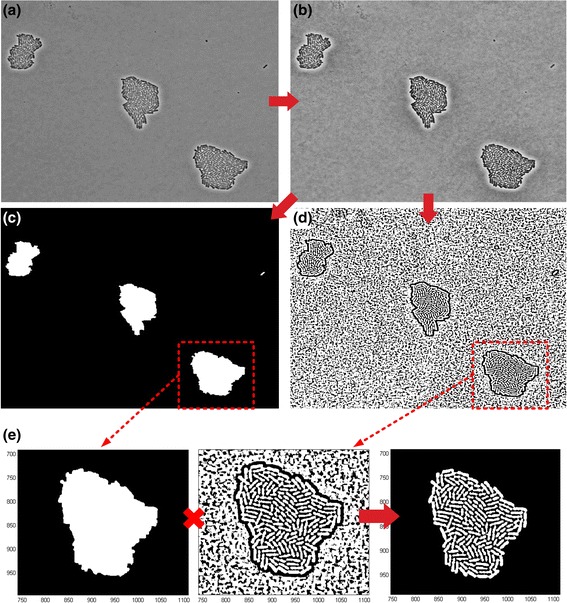
Image preprocessing and Colonies Segmentation. a Input image with three colonies (SalPhase movie). b Contourlet based denoising and adaptive histogram equalization used to sharpen cell edges. c Colony masks created using morphological filtering, Otsu’s global thresholding and Canny edge detection; they are used to separate colony regions from image background so that each colony can be processed separately in the pipeline (divide-and-conquer). d Adaptive thresholding is used to remove the colony’s local background pixels. e Multiplication of the image generated by adaptive thresholding with the corresponding extracted mask (Colony in the red rectangle) removes the noise (existing locally in the colony) and the artifacts (produced by the adaptive thresholding algorithm) while revealing cell objects inside the colony

After preprocessing, our colony segmentation method creates a binary mask used to separate each colony from the image background. We first apply a mathematical morphology operation (rolling ball method) [37] to estimate the image background. Then we use Otsu’s global thresholding [38] and Canny’s edge detection algorithms [39] to create a binary image (global background mask) outlining as precisely as possible the region of each colony, regardless of its size (see Fig. 1(c)).

After completing this task for each image frame, we track each colony and extract its properties (e.g. number of cells, total area, location of the colony’s centroid etc.) in the time-lapse movie. Specifically, in order to determine the correspondence of two colonies in two consecutive frames, we check whether the centroid of a colony in the previous frame lies inside the bounding box of a colony in the current frame, and if so this colony is matched. If a colony in the current frame matches to no colony in the previous frame, we treat it as a new one, since we consider it possible for a colony to enter to the microscope’s field of view while the experiment is running. When two or more colony centroids of the previous frame lie inside the bounding box of the same colony in the current frame, the algorithm identifies that these colonies have merged. This capability is important since in a large bacterial community colonies can merge or move out of the field of view. Keeping track of colonies as they grow and merge is important not only for archiving their time varying properties but also for knowing the colony from which each individual cell has emerged i.e. the subpopulation to which it belongs to, without using any fluorescent markers. To the best of our knowledge, our divide and conquer computational approach is the only one that can track multiple subpopulations (colonies) that may merge, in addition to single-cells, in cell movies.

Single-cell segmentation algorithm

Having defined a colony’s region as accurately as possible, we can now “zoom in” and detect individual cells effectively. A visual overview of the whole segmentation approach is provided in Fig. 2.

Fig. 2.

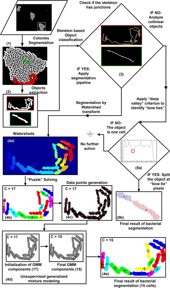
Overview of the cells segmentation method. (1) Colonies segmentation. (2) Objects identification inside a colony. (3) Skeleton based object classification; (4) Complex object segmentation: 4a) Watershed algorithm application, 4b) “puzzle solving” step, 4c) new dataset generation, 4d) unsupervised Gaussian mixture modeling, 4e) final result of bacterial cells segmentation. (5) Collinear object segmentation: 5a) Application of the “deep valley" criterion to identify “bow tie” points, 5b) final result of bacterial segmentation. At step (3), there is a bifurcation leading to different processing routes based on the object's classification. See text for details

From colonies to cell objects

Despite the applied preprocessing, each colony may still contain local background pixels due to large illumination variations (e.g. see Fig. 1(b)). To overcome this problem, we use adaptive thresholding [37] to separate cells from the non-uniformly illuminated background (see Fig. 1(d)). We remark that this type of background variability is typical for images acquired by optical microscopes (either bright field or phase contrast) but not for images acquired using confocal laser scanning microscopes (CLSM) [40]. Nevertheless, the adaptive thresholding method used here has no negative effect on CLSM images. However, as illustrated in Fig. 1(d) adaptive thresholding introduces "salt and pepper" noise, so in order to eliminate it we multiply the processed image with the global background mask. The result is an image with the global background removed and the local noise inside each colony suppressed (see Fig. 1(e) for the 3rd colony of SalPhase movie).

However, the individual cells inside the colony may not be fully separated (segmented) at this stage. We rather observe that the colony is partitioned into "cell objects", where each object is a set of cells "touching" each other (see Fig. 3(a) for examples). The union of these objects covers all cells in the colony and their pairwise intersection is empty (every single-cell belongs to one and only one object). In the colony of Fig. 3 (a) three objects have been colored for demonstration purposes, one green and two red. The green is a so called collinear object while the two red ones are considered complex objects. To determine an object’s category (collinear vs. complex) we developed a divide-and-conquer approach where we analyze each object individually. First, we compute the object's skeleton as presented in [37] (refer to Fig. 3 (b-d)). Then, if the skeleton has "junction points" (i.e. pixels that have more than two pixel neighbors [37]) the object is considered complex. On the other hand, if we find no junction points, the object is either a single-cell or a cascade of single-cells (collinear object), see Fig. 3 (c).

Fig. 3.

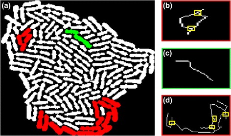
Cell Objects extraction and classification. a Each colony is an ensemble of cell objects corresponding to one or more “touching” cells; e.g. see three cell objects marked with color. We first extract the skeleton of each object and classify it as complex (red) or collinear (green) according to the presence (or absence) of skeleton junctions (i.e. skeleton pixels with more than two neighbors). b The skeleton of the smaller red object has two junctions (marked with yellow boxes) so it is classified as a complex object. c Colony object with no junctions (green) classified as collinear object. d A complex object (large red) with four junctions. See text for details

Collinear object analysis

In order to ascertain if a collinear object corresponds to a single-cell or a series of connected single-cells (i.e. a cell "sausage" like structure) we developed a simple algorithm based on the observation that the shape of a bacterium at the fission stage [41] resembles that of a bow tie (refer to Fig. 4 (a)). The algorithm searches for "bow tie points" by computing the Euclidean distances [42] of all pairs of diametric pixels (antipodal) lying on opposite boundaries with respect to the object’s centerline. Then, it identifies significant local minima (Fig. 4 (c)) of the distance curve, meeting the following criteria:

Fig. 4.

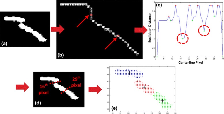
Collinear objects analysis - "Bow ties" identification. a Extracted collinear object. b Skeletonized object with skeleton pixels numbered. The red numbers mark the “bow tie" locations on the centerline. c Distance curve of the object: To construct it we form pairs of opposite-side diametric boundary pixels (w.r.t. the skeleton) and compute their Euclidean distance (local width). Then we search for “deep valleys” (i.e. significant local minima relative to neighboring local maxima (marked with red circles for illustration purposes) and, (d) we split the object at bowtie points (marked by red dashed lines for illustration purposes), that correspond to the deep valley positions in (c). e The collinear object is segmented into three single-cells

localMin/leftLocalMax ≤ T and localMin/rightLocalMax ≤ T

where localMin is the local minimum and leftLocalMax and rightLocalMax are the local maxima lying around the local minimum. Such local minima (if they exist) are called “deep valleys” (Fig. 4 (c), indicated by red circles). Intuitively, T is the ratio of the minimum to maximum width (i.e. the distance of diametric pixels with respect to the object’s centerline from the center of the one pole semi-circle to the center the other pole semi-circle) measured at the frame before the first cell division. The value of threshold T is automatically set by the pipeline and is usually in the range [0.65, 0.75]. When the algorithm identifies the existence of deep valleys, we split the object into discrete cells at these locations (marked with red dashed lines in Fig. 4(d)), that correspond to the deep valley points on the centerline (the x-axis in Fig. 4(c)) because the centerline pixels are ordered (see Fig. 4(b)). Otherwise the collinear object remains intact and is considered as a single-cell. Finally, for each segmented cell, we identify its centroid by averaging its pixel coordinates (see Fig. 4(e)).

Complex object analysis

Complex objects are treated differently than collinear objects. First we use the watershed transform [43] to estimate how many cells are possibly "hidden” inside a complex object. We determine the centroids of extracted watersheds and consider them as initial estimates for the centroids of potential cells in the complex object (see Fig. 2 (4a)). However, a well-known problem of the watershed transform is that it favors over-segmentation [44]. So, we apply the “deep valleys” algorithm again, but in a slightly modified way. This time we need to decide whether we should merge erroneously over-segmented cell fragments, so as to avoid generating false positive cells. Fragments in the neighborhood of a given fragment are examined to determine if they should be merged with it or not. Two touching fragments can be merged if there is no bowtie point between them, identified using the deep valleys criterion. If a potential cell (watershed fragment) can be merged with more than one neighboring cells, then the merging that leads to maximum solidity is chosen. Solidity is defined as the ratio of the resulting area to the resulting convex hull area, based on the conjecture that elementary objects, i.e. well-formed single-cells, tend to have a solidity value close to one. Moreover, the new object (after the merging) is inserted into a processing queue in order to be further examined whether it should be merged with another watershed fragment. We call this iterative procedure “puzzle solving” algorithm (see Fig. 2(4b)).

In order to outline the detected cells as accurately as possible and improve the segmentation result, we apply a machine learning method based on Gaussian Mixture Modeling (GMM) [45]. In [45], we have shown how to transform image pixel intensities to a properly constructed set of data points before applying GMM to identify protein spots in a 2D electrophoresis (2DGE) gel image. In our case, pixel intensities provide no information about cell structure since they follow a uniform distribution (see Fig. 5 (a)). So we use the minimum distance from cell boundary (Euclidean distance transform [46], see Fig. 5 (b)) as the basis for data points generation. Specifically, we consider each pixel of the object acting as a data points generator in its neighborhood (refer to Fig. 6). The total number of data points, N, to be generated by random sampling and used to represent each object will be proportional to the number C of its estimated cell centroids. These N data points are apportioned to the pixels of the object according to each pixel’s Euclidean distance from the object’s boundary, meaning that more internal pixels will be allowed to “throw” more data points in their neighborhood. Following this data generation scheme, the pixels closer to the object’s centerline belong to it with higher probability than the more distant ones.

Fig. 5.

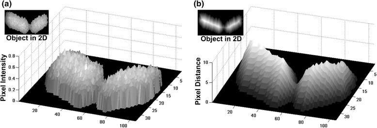
Distance transform. a Cell object depicted in 3D; the image pixel intensities are shown in the z-axis. b Same object's distance transform in 3D; the distance values are shown in the z-axis. It is obvious that the distance transform [40] smoothens object abnormalities while sharpening the valley between the two cells comprising the cell object

Fig. 6.

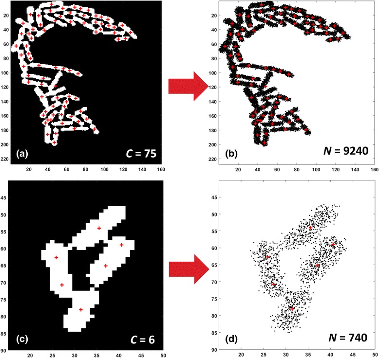
Complex object Analysis - Generation of a dataset representing the object. a A very complex object (large number of cells) including potentially 75 single-cells. b Data points generation for the object in (a) by random sampling (see text for details), 9240 data points generated. c A less complex object with only 6 potential cells. d Data points generation for object in (c), 740 data points generated. The number of generated data points is proportional to the number of the complex object centroids, thus it depends on the object’s structural complexity (number of potential cells included). Also, more data points are randomly “thrown” around the cells’ medial axes, so as to best represent cell structures (see text for details)

We may think of this process (moving from pixel intensities to data points) as a reverse engineering step where the resulting data points represent best the bacterial shape. Specifically, a pixel i located at coordinates (x _i , y _i ) with distance d _i acts as a data generator using a 2-D Gaussian model N(μ, Σ ) with center μ = (x _i , y _i ). Finally, we get a GMM [47] having as many Gaussian components as the number of the pixels M in the object. Each component has a mixing coefficient proportional to its distance value and equal to:

π(i) = d _i/∑^M_j = 1 d _j.

So for each pixel i of the object we draw N∙π(i) data points from a 2-D Gaussian distribution which is centered at the pixel’s location μ = (x _i , y _i ) with diagonal covariance matrix Σ having its elements set to 0.3. The variance value (0.3) was selected to be smaller than 0.5 (half-distance between neighboring pixels) in order to ensure that data points generated by the model (representing “cell structure”) will be distributed in a manner that guarantees that their abundance reflects the distance, thus preventing the generation of “hills” of data points in-between pixel locations. This variance value was determined by experimentation and is kept fixed throughout the analysis, irrespectively of the image modality.

As mentioned before, the number N of data points generated for a complex object is proportional to the number of the estimated candidate cell centers C it may contain. In particular we use

$$N=\frac{\mathit{1}}{\mathit{2}}C\frac{\mathit{CellLength}\times \mathit{CellWidth}}{\mathit{CalFacto}{r}^2}\text{,}$$

where CellLength is the expected cell length, CellWidth is the expected cell width of the species under examination and can be estimated from literature. For example for Salmonella S. Typhimurium the width (diameter) range considered is [0.7, 1.5] μm (so we chose CellWidth = 1.1 μm), and in length range is [2, 5] μm (so we choose CellLength = 3.5 μm) based on literature [48]. Let us remark that even if these cell size parameter values are overestimated the approach will suffer only from a performance loss (e.g. by using a larger than needed N value). Moreover, CalFactor is the spatial calibration factor of the experiment’s microscope used to convert the size of an image object from pixels to physical units (μm).

Using an N value that is proportional to C was a deliberate choice because the number of identified candidate centers can act as an object’s complexity indicator approximating the number of single-cell structures expected to be present in a complex object's region. So, if a complex object contains a lot of candidate centers, it is justified to “throw” more data points (use a larger N) in order to capture adequately the underlying structure of the different single-cells included in it. As shown in Fig. 6, the generated data set for the object with the six candidate centers (Fig. 6(c)) "spent" less data points (Fig. 6(d)) than the object with the 75 candidate centers (see Fig. 6(a) and (b)).

After generating the data points we associate each one of them with its closest center using Euclidean distance [42] and nearest neighbor classification [49]. Starting with this initial assignment, we can determine the initial parameters of a 2-D GMM having C components (as many as the estimated cell centroids in the object) and compute the log-likelihood of each data point to belong to this initial mixture model:

$log\mathrm{p}\left({\mathbf{y}}^{\left(i\right)}\left|\Theta \right.\right)=log{\displaystyle \sum _{\mathrm{m}=1}^C{w}_m\mathrm{p}\left({\mathbf{y}}^{\left(i\right)}\left|{\theta }_{\mathrm{m}}\right.\right)}$,

where Θ≡{θ ₁, …, θ _c, w ₁, …, w _c} is the complete set of mixture model parameters and w _m are the mixing coefficients.

The next step is to apply Finite Mixture Modeling (FMM) [50] in two dimensions (see Fig. 7). An important issue in mixture modeling is the selection of the proper number of components to use. With too many components the mixture may overfit the data, while with too few components it may not be flexible enough to capture the true underlying reality [50, 51]. In our case, this would translate to a solution with either more or less components than the actual number of cells present inside a complex object. In order to overcome this difficulty we apply a modified Expectation Maximization (EM) algorithm [50] which also employs the Minimum Message Length (MML) criterion [51] for best model selection. However, since the EM with MML is computationally expensive we first apply the "puzzle solving" algorithm to estimate the initial number of components properly i.e. start the iterative algorithm at a number not too far from that of the best model. Using the MML criterion ensures that the best model will not end up being an unnecessarily complex one unless if it pays for itself. Therefore, it is possible that the best model may end up containing less than the initial number of C components (see Fig. 7). At the end, it is possible that some circular object fragments may still remain isolated and not merged with the cell they really belong to, especially when analyzing low resolution cell movies. To overcome this difficulty, we check if a fragment’s area is under a pre-specified threshold

$$A=\frac{\mathit{1}}{\mathit{4}}\pi \cdot {\left(\frac{\mathit{CellWidth}}{\mathit{CalFactor}}\right)}^2$$

Fig. 7.

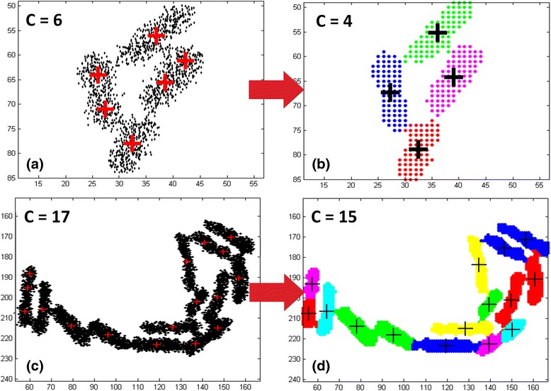
Cells segmentation - Best Gaussian Mixtures Model fit. Initialization of Gaussian mixture model parameters is performed after associating data points to cluster centers using nearest neighbor classification. For the complex object in (a) we have initially C = 6 components (clusters) in the mixture and for the model in (c) C = 17 components. We then apply the Expectation-Maximization (EM) algorithm and use the Minimum Message Length (MML) model selection criterion to identify the number of mixture model components that produces the best model fit. In (b) this results to a reduction of clusters from 6–4, and in (d) from 17–15. Each component in the final model represents a segmented single-cell (see text for details)

determined automatically by the pipeline using the pre-specified parameters. Fragments with area less than A are merged with the "touching" neighbor that maximizes the resulting object's solidity after the merging (as mentioned in the "puzzle solving" step of the analysis) otherwise they remain intact and are considered to be undersized single-cells. Intuitively, considering a cell's projection on the plane as a curved parallelogram with two attached semi-circles (poles), its area must be at least the area of the two cell poles, i.e. the area of a circle with radius equal to one half of the expected cell's width as in A.

Lineage tree construction

A cell in a time-lapse movie frame can: 1) proliferate, 2) divide, and 3) die or disappear from the microscope’s field of view. In order to construct the lineage of a single cell, first we have to segment the cells of each colony efficiently and then we have to track the colonies and their cells along consecutive frames. In order to track cells in overcrowded bacterial time-lapse movies, we have developed an algorithm inspired by motion estimation techniques used for video compression [52] which also follows a divide-and-conquer strategy. Our cell tracking algorithm will not be discussed here since it has been published in [53].

Single-cell and colony properties extraction

For each colony, we compute growth curves in terms of the colony’s area (either in pixels or in micrometers) or in terms of cell population (cell counts). In addition, we extract numerous properties at the single-cell level. We divide single-cell properties into two categories: cell attributes and cell life attributes. Attributes are cell properties changing with time, characterizing each cell at each frame of the time lapse movie. For example, cell attributes that we track are: area, fluorescent protein quantity (if any), major axis length (length), minor axis length (width), distance from the colony’s centroid etc. On the other hand, cell Life attributes are statistics of attributes (e.g. min, max, average, median, standard deviation) characterizing a cell’s whole life "trajectory", i.e. from its birth to its division. In addition, elongation (i.e. how much a cell has changed length before it divides) and division time (i.e. the duration of a cell’s life) are life attributes too. Additionally, given an attribute’s evolution (time-series) we can estimate life attributes e.g. estimate an individual cell’s elongation rate by fitting an exponential model to the cell’s trajectory. All these properties are estimated and exported (stored) to a bio-database for each individual cell and time frame in the movie. Moreover, several useful visualizations can be produced for displaying the computed cell attribute values directly using color on top of the input time-lapse movie videos (refer to Additional files 4, 5 and 6) or on top of a colony’s lineage tree or divisions tree as it will be demonstrated in the Results and Discussion section.

Download video file ^{(792.7KB, mp4)}

Additional file 4: Computed cell length overlaid on SalPhase time-lapse movie. (MP4 792 kb)

Download video file ^{(6.6MB, mp4)}

Additional file 5: Multi-SalPhase time-lapse movie; cell length visualization after segmentation. (MP4 6740 kb)

Download video file ^{(517KB, mp4)}

Additional file 6: SalPhase time-lapse movie; color indicates cell generation index as determined by the cell tracking algorithm. (MP4 516 kb)

Implementation

The pipeline of algorithms presented here has been coded in Matlab version R2015b [54]. We used extensively the image processing, statistics and machine learning, wavelet and curve fitting Matlab toolboxes. All presented results were obtained using a desktop computer with Intel Core i5-3350 processor running at 3.10 GHz, 8GB RAM, under Microsoft Windows 7 professional operating system. The current implementation is not optimized for performance. Nevertheless, a discussion of the trends of its running time is provided in Supplementary Material section 5 (see Additional file 1). Due to the divide-and-conquer strategy followed that breaks large problems into smaller subproblems, we expect that the use of parallel processing can significantly accelerate the analysis. All post-processing capabilities are also implemented in Matlab, so as to enable users to interact with the data produced using simple function calls. The authors' intention is to complete the software integration and performance optimization, add a proper user interface and then make the software accessible to the systems biology community. The emphasis of this methodology paper is on the innovative methods integrated in the BaSCA pipeline and not on the software architecture and implementation.

Results and discussion

Comparison to the state of the art

In order to compare the segmentation performance of the proposed pipeline with state-of-the-art methods, we chose software packages that are extensively used by different labs worldwide to analyze cell movies and that have been referenced in several studies [55–66]. Moreover, we analyzed representative still (single) frames provided by the state-of-the-art software packages at their websites (see Materials), as well as two more images, a frame from our SalPhase movie (frame 74) and a frame from our Multi-SalPhase movie (frame 78). The Recall, Precision and F-measure was computed for each dataset and method used in the comparative evaluation.

The table in Fig. 8 summarizes the evaluation results. Dashes (tildes) in table entries indicate that the specific method did not return results (or gave very low quality results) respectively. CellTracer was able to analyze only the frame downloaded from the CellTracer’s movie. TLM Tracker performed well with images having only one small-size colony in the field of view (such as in CellTracer’s and Schnitzcells’ images). Oufti and Schnitzcells were the most robust among the state-of-the-art methods, returning results for all images. The proposed pipeline exhibited a notable F-measure advantage for all imaging modalities and datasets used; its F-measure remains very high (over 96.7%) even for images with multiple overcrowded colonies in the field of view. Moreover, it outperformed the other approaches even when using images from their own repertoire. Only BaSCA returned near perfect results (F-measure of 99%) for the SalPhase movie, achieving perfect recall and an almost 10% higher F-measure than Oufti. In Multi-SalPhase, a movie containing many overcrowded colonies in the field of view, BaSCA achieved F-measure 96.7% in comparison with the state-of-the-art software, Schnitzcells which achieved 90.9%. Oufti did not provide reliable segmentation results for this dataset. The results of the comparative evaluation for all methods along with the used parameterizations and input images are provided for each dataset as Supplementary Material (see Additional file 7).

Fig. 8.

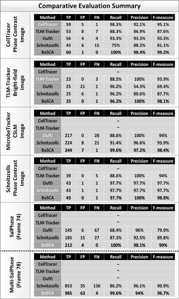
Comparative Evaluation Summary. Each section of the table reports the evaluation results for an image suggested by one of the methods under comparison. The table columns list the true positives (TP), false positives (FP), false negatives (FN), as well as the Recall, Precision and F-measure achieved by each method. SalPhase frame 74 and Multi-SalPhase frame 78 were used to assess the performance of the methods on images with dense and overcrowded colonies. Dashes (-) indicate failure to return results for a specific dataset. Tildes (~) indicate very poor performance. The proposed method (BaSCA) achieved consistently very high F-measure (≥97.3% for all cases), suggesting that it is robust across imaging modalities and datasets produced by different labs. (Refer to Additional file 1: Figures S1-S5 for the detailed segmentation results)

One of the main contributions of this work is that, in contrast to the state-of-the-art methods, BaSCA can segment successfully images with multiple overcrowded colonies as they grow and merge, potentially with thousands of bacteria in a field of view (see Additional file 5 providing a video with the segmentation results of Multi-SalPhase movie). Figure 9 illustrates this fact. Segmentation accuracy when analyzing frames with overcrowded colonies is almost as high as in non-overcrowded frames. Recall remains over 98%, precision over 91% and the F-measure over 94%. Due to its high segmentation robustness, BaSCA can estimate several time-varying colony and single-cell level properties accurately fulfilling the expectations of image driven single-cell analytics for predictive microbiology.

Fig. 9.

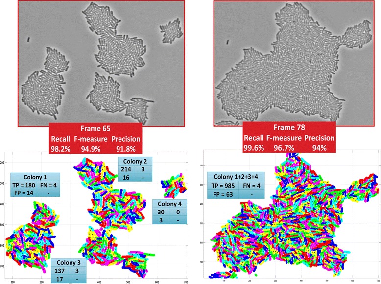
Segmentation of overcrowded and merging colonies. The four colonies in frame 65 of movie Multi-SalPhase (left) are merged several frames later (frame 78, right). Top panels: input image frames. Bottom panels: Segmentation results: The cyan boxes report the TP, FN and FP for each colony. The red boxes summarize the evaluation measures for each frame. Pseudo-colors are used to make cell boundaries visible. BaSCA achieves both high recall and high precision and an F-measure over 94%

We should emphasize that the state-of-the-art software packages used in the evaluation require a different parameterization for each imaging modality. Thus, we had to perform extensive experimentation to find the most appropriate parameter settings for each dataset before the evaluation (see Additional file 7 for the parameterization of each software and datasets). This is a laborious task that requires the user has knowledge of image processing concepts e.g. to select filter types, set parameters, select segmentation methods etc. (refer to Additional file 1: Table S1). In contrast, the parameterization of BaSCA is trivial. All parameters used by the pipeline are set automatically once the user inputs the spatial calibration factor, image modality and the expected value for the average cell length and cell width (diameter) of the species under examination as discussed in Methods. Eliminating the need for an elaborate parameterization was a deliberate choice since our objective was for the pipeline to be used trivially by microbiologists with no expertise in image analysis and to be easy to integrate into larger service workflows for high throughput single-cell analytics and systems biology.

In summary, BaSCA extends the current state of the art by being: (a) more accurate, (b) more versatile since it can process datasets produced using different microscopy types/imaging modalities and return trustworthy results, (c) high throughput, automated, without requiring a human in the loop, and (d) able to analyze efficiently and at many levels cell movies with multiple colonies that grow and merge, resulting in overcrowded bacterial communities with thousands of cells in the field of view.

Comparison to the ground truth

In Fig. 10(a), we present a summary of the comparison of our pipeline's results versus the ground truth for the whole SalPhase movie (86 frames). We observe that BaSCA achieves a recall over 99% and precision over 96%. Overall it achieves a very high F-measure of 98%. In this movie we have accounted correctly for 6856 out of the 6895 true cells and made only 263 errors, mostly false positives. The results per frame and per colony are provided in Additional file 8. It is significant that the proposed methodology achieves a very high F-measure score (>93.27%) in all frames, which proves its segmentation robustness. The segmentation results for the frame with the lowest F-measure (frame 63) are provided in (Additional file 1: Figure S1). The majority of the errors appear during the exponential phase (after the 8^th cell generation); beyond this point the colonies start growing in the 3^rd dimension. In summary, the results suggest that the developed pipeline remains both very sensitive and very precise as long as colonies maintain their 2-Dimension structure.

Fig. 10.

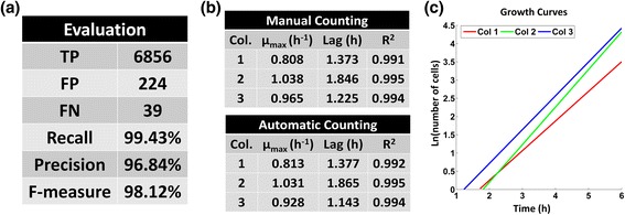
Growth rates - Evaluation w.r.t. the ground truth. a Evaluation results summary for the SalPhase movie (86 frames). The developed pipeline achieves a very high F-measure above 98%, (b) Comparison of manual vs. automatic BaSCA counting for the three colonies of the SalPhase movie by fitting a Baranyi and Roberts model [43]; the kinetic parameters of microbial growth are almost identical, (c) Automatically estimated growth curves of the three micro-colonies in the dataset

BaSCA can provide, in a high throughput no-human in the loop manner, accurate data to support predictive modeling for systems microbiology. In order to demonstrate this important capability we also fit the primary model of Baranyi and Roberts [67] to the growth curves of each colony in the SalPhase movie. This mathematical model is commonly employed by microbiologists to estimate growth kinetic parameters of a cell population in a given environment. The kinetics parameters of the population are its lag time (λ) and the maximum specific growth rate (μ _max). To describe the abrupt transition of the observed cell growth from the lag to the exponential phase the values of the model parameters m and n were fixed to 0 and 20 respectively as in [13]. In Fig. 10(b), we present the estimated kinetic parameters for the three growing colonies in the SalPhase movie extracted using manual and automatic cell counting. We can see that the kinetic parameters using the ground truth (manual counting) are almost identical to those estimated using automated BaSCA counting. In Fig. 10(c), we observe that although in the movie we have three colonies emanating from three single-cells and growing concurrently in the same micro-environment, their growth dynamics are quite different as also shown in [13]. Consequently, it becomes apparent that our analysis pipeline not only provides trustworthy results without any human involvement, but also provides a useful tool for characterizing the stochasticity exhibited in colony dynamics. This can accelerate predictive microbiology studies that try to elucidate the functional role of stochasticity [3, 4, 13–15] and how it is affected by community effects [6, 7, 16, 17].

Single-cell analytics and visual exploration

Accurate and automated image analysis for large size bacterial communities enables single-cell analytics and high throughput systems microbiology. In Fig. 11, we present the Entity-Relationship (ER) model [68] of a database schema that supports the image-driven single-cell analytics system developed. In this bio-database representation of a cell movie, we capture essential information regarding the settings of the underlying experiment (Experiment table), and the time lapse microscopy characteristics (Frame table). In addition, we store a plethora of properties extracted by the image analysis for each colony in the field of view (Colony Table), as well as for each segmented single-cell of each colony (Cell Instant Table and Cell Table). Specifically, we store single-cell properties that may change at every time instant (cell attributes) as well as properties that characterize a cell’s whole life span, from birth to division time (cell life attributes). For example, in the Cell Instant Table we store extracted cell attributes (e.g. cell area), while in the Cell Table, we store the estimated/measured cell life attributes (e.g. the cell's elongation, division time etc.). The bio-database stores the "big data" that result from the analysis performed at different levels (frame, colony, and single-cell), providing essential meta-data for the experiment that can accompany the imaging data, and/or used in lieu of the imaging data in subsequent analytics and modeling efforts. This unique aspect of BaSCA not only enables image-driven systems microbiology, but provides a mechanism for reducing the cell movies massive data down to the useful information that can be exploitable by downstream processes. This is a very useful feature for building repositories of annotated cell movies with meta-data that can be searchable and usable in systems biology workflows over the internet.

Fig. 11.

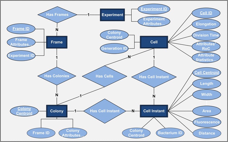
Single-cell analytics database ER-Diagram. Organization of the database storing information about the experiment that generated the cell movie (Experiment table) and the time lapse microscopy characteristics (Frame table). In addition, we store the image analysis generated information for each colony in the field of view (Colony Table) and for each segmented cell within each colony. Specifically, single-cell attribute values changing at every time point are stored in the Cell Instant Table, while cell life attributes that characterize the whole cell life trajectory are stored in the Cell Table. The database summarizes the cell movie image analysis completely and can be used for downstream single-cell analytics and visualization. Moreover it forms the basis for building repositories of cell movies under different conditions for large scale high throughput systems microbiology experiments

In Fig. 12, we present a visualization of the cell segmentation results. We observe (Fig. 12(a)) that segmentation is accurate since the overlaid green contours outline the real contour of each cell. As a consequence, we can have confidence that we can measure cell attributes correctly. In Fig. 12(b, we show how a cell attribute (e.g. cell length) can be visualized using BaSCA. The different colors represent cell length (in micrometers, μm), in the range indicated by the color bar. This kind of simple visualization allows the user to distinguish spatial patterns, or even focus on specific bacteria according to the chosen cell attribute of interest. Moreover as a byproduct of the multi-scale image analysis BaSCA can generate time-lapse movies of segmented growing colonies that animate the visualization of any extracted cell attribute of the user's choice. Additional files 4 and 5 provide video animations of the space-time evolution of the cell length attribute for the SalPhase and Multi-SalPhase cell movies, respectively.

Fig. 12.

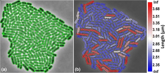
Cell attribute visualization. a BaSCA segmentation results for colony 3 of the SalPhase movie (frame 86). Green curvatures mark the contours of segmented cells. b Cell length visualization using color, overlaid on each segmented cell. Movies of cell length visualization are provided in Additional file 4 and 5 for SalPhase and Multi-SalPhase datasets respectively

Automated lineage tree construction of large-size over-crowded colonies is also an important requirement for high throughput systems microbiology. CellTracer, TLM-Tracker and Schnitzcells support lineage tree construction; however, they are limited to colonies with a small number of cells and do not exploit lineage trees as drivers for single-cell visual analytics [53].

Our methodology allows users to exploit lineage tree construction to visualize the evolution of single-cell attributes extracted from the automated image analysis of time-lapse movies. For example, we can visualize on top of the lineage tree the evolution of single-cell area in a colony (see Fig. 13), and thus inspect easily how it tends to change during the cells' life span. Moreover, we can visualize the evolution of cell life attributes e.g. their division time. We achieve this by constructing a condensed circular tree, called divisions’ tree, containing as nodes only the cell division events. In Fig. 14, we use Tulip [69] to visualize on the divisions tree, the cell division times of the 3rd colony cells of the SalPhase movie. This is a very useful visual analytics feature since it can help us to quickly assess how cell life attributes evolve across generations under different experimental conditions.

Fig. 13.

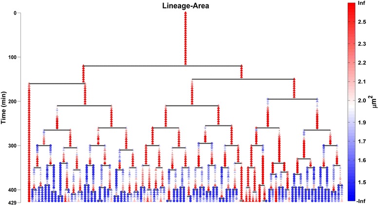
Single-cell attribute evolution visualization on the lineage tree. The lineage tree of colony 1 (top left) of the SalPhase movie. The area attribute is visualized using color on the tree for every cell and time instant (frame) of the movie. Triangular (circular) shape node glyphs are used for time instants that a cell lies in the colony’s boundary or within the colony respectively. Any cell attribute available in the database produced by the image analysis can be visualized in the same manner

Fig. 14.

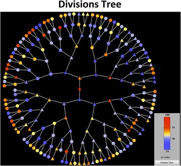
Cell life attribute visualization on the cell divisions tree. A circular tree of cell divisions (root cell in the middle) for colony 3 of the SalPhase cell movie. Colors represent here division times (min) as indicated by the color bar. We can easily assess visually how division times vary along tree branches (cell clones) and tree levels (cell generations). Triangular (circular) nodes represent cells that lie on the colony’s boundary (within the colony) respectively. Any cell life attribute available in the database produced by the image analysis can be visualized in the same manner. The Figure was created using the Tulip software package [67]

Image-driven single-cell analytics support systems microbiology

Using the results of the analysis at the single-cell level, i.e. cell attributes and cell life attributes, allows us to verify literature results and formulate interesting new hypothesis for future research. For example, given the extracted lineage tree of a colony and the estimated length of every cell at every time instant, we can fit to each cell's length trajectory (time series) an exponential model [70, 71]. Specifically, let us consider as in [71] a single-cell length model of the form l _t = l ₀ ⋅ e ^kt, where l ₀ is the birth length of a stalked cell and k is its growth rate (cell elongation rate). In this way we can capture the growth characteristics of each cell and estimate its personalized kinetic parameters. In Fig. 15(a) we provide the growth curves of each individual cell of the SalPhase movie estimated using non-linear least squares [72]. We observe that single-cell growth kinetics exhibit great variability, something that cannot be observed by population based experiments. In Fig. 15(a) we provide the average single-cell growth curves for each colony of the SalPhase movie. We notice that average growth curves vary among colonies of the same movie that grow in the same micro-environment under the same experimental conditions. Clearly, colony 3 exhibits less heterogeneity (smaller variance) than the rest of the colonies. Single-cell analytics enables zooming in and extracting useful information regarding subpopulation characterization for any cell attribute of interest among the many extracted by BaSCA.

Fig. 15.

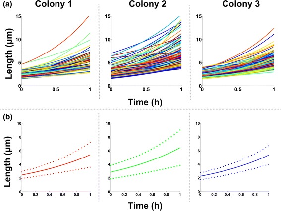
Single-Cell Exponential Growth curves. a Single-cell growth curves estimated from the image-analysis data after fitting an exponential individual cell length model (see text for details). Different colors represent different single-cell lifespan trajectories. b Average cell growth curves of each colony (solid lines). Dashed lines represent one standard deviation above and below the average curve. We observe that cell growth exhibits considerable variability among colonies, and cells within the same colony (SalPhase cell movie)

Single-cell analytics also allows characterization of intra and inter-colony as well as intra and inter-generation variability of cell life attributes. In Fig. 16, we present the best gamma distribution fits of the single-cell elongation rate k, division time T, and cell length at division l _f per colony (cells from 3^rd to 8^th generation were pooled, SalPhase movie). The estimated best model parameters are provided in (Additional file 1: Table S2). We observe that the cell life attribute distributions of the 3rd colony have a lower variance than the rest of the colonies. Intuitively, this suggests that the cells of the 3rd colony grow and divide more synchronously across generations. This is actually confirmed by examining the cell generations movie, i.e. a version of the SalPhase movie in which we have colored cells according to their generation index at any instance as determined by our automated tracking and lineage tree construction algorithms (see generations movie in Additional file 6). Such subpopulation investigations would be impossible without a single-cell analytics focus; our image-driven single-cell analytics approach enables zooming-in and characterizing cell properties at any desirable level of community organization, in space (colonies) or in time (subtrees of the lineage tree).

Fig. 16.

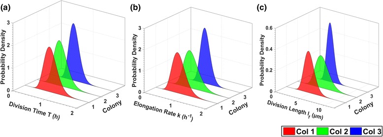
Life attributes variability per colony. Gamma distributions (best fit) of (a) the cell division time T, (b) the cell elongation rate k, (c) the cell division length l _f for colonies 1, 2 and 3 (SalPhase movie). The proposed methodology allows us to characterize the variability of cell life attributes across colonies. Similar analysis can be performed for any life attribute available in the database after image analysis using BaSCA

In Fig. 17, we provide the best fit Gamma distributions of the aforementioned cell life attributes, but now per cell generation (cell data from the three colonies are pooled, SalPhase movie). We chose the Gamma distribution because the histograms of the aforementioned attributes have similar shape (skewness) to it (in Additional file 1: Figure S2 and Figure S3). Moreover, the gamma distribution is a flexible two-parameter distribution that belongs to exponential family and is used to model physical quantities that take positive values in microbiology, such as the cell division time (as in [14, 73]), the cell elongation rate (as in [73] and cell division length (as in [71]). The estimated parameters are provided in (see Additional file 1: Table S3). In Fig. 17(c) we observe that there is a trend towards lower mean and smaller variance for the cell division length attribute as the generation index increases. Single-cell analytics offer the capability to quantify the stochasticity and examine inter and intra-generation variability by estimating epigenetic correlations of single-cell attributes.

Fig. 17.

Life attributes variability per generation. Gamma distributions (best fit) of (a) the cells division time T, (b) the cell elongation rate k, and (c) the cell length at division l _f for the 3^rd to the 8^th generation of cells of the SalPhase movie (cells from all colonies pooled). By delving into each generation’s individuals we can characterize a life attribute's intra and inter-generation variability (stochasticity). Similar analysis can be performed for any life attribute available in the database after image analysis using BaSCA

However, the division length does not correlate explicitly neither with the elongation rate nor with the division time, since the estimated Pearson correlation coefficients are very low for both cases (r = 0.2 and r = 0.01, respectively for the SalPhase movie). This is a rational result because cells growth depends both on the elongation rate and on the life span (i.e. division time) of the cell simultaneously, as shown in [70, 71], factors which are both epigenetic information inherited by the cell's progeny as mentioned in [11, 12]. So, we cannot assume that a cell that is going to live longer, i.e. that will have higher division time, will necessarily become lengthier too, given a specific birth length. In order to demonstrate this we computed the correlation coefficients of cell life attributes estimated by our image analysis and compared them to corresponding coefficients estimated in [70] where E. coli cells were grown individually in microfluidic devices. Specifically, we considered single-cell elongation, defined as $E=\mathit{log}\frac{l_f}{l_0}=k\cdot T$, and computed its correlation to the natural logarithm of the cellular birth length (ln(l ₀)). The Pearson correlation coefficient was found to be r = -0.44 (see Additional file 1: Figure S4(a)), and this is in striking accordance to what was found in [70] (see Fig. 2 of [70]). The anti-correlation between elongation and cell birth length (see Additional file 1: Figure S4(a)) is entirely due to a modulation of the division time, with the elongation rate appearing to be independent of birth length (see also Additional file 1: Figure S4(b-c)) as it was also found in [70]. It is also interesting that the correlation coefficients of (ln(l ₀)) to cell division time (T) and elongation rate (k) we found through single-cell analysis match closely the values reported in [70] (see Additional file 1: Figure S4(b-c)). These findings verify that BaSCA algorithms quantify accurately single-cell properties when analyzing bacterial colonies growing in microenvironments accounting for the community dynamics.

Conclusions

We presented BaSCA, a novel Bacterial image analysis driven Single Cell Analytics pipeline which enables the high throughput analysis, down to the single-cell level, of complex time lapse cell movies with many colonies and potentially thousands of cells in the field of view. The results presented demonstrate its robustness and universality. In contrast to other methods, BaSCA is fully automated and does not require users to be familiar with image processing concepts and/or provide an elaborate parameterization to get good results any time a new movie is analyzed. BaSCA not only improves the accuracy of segmentation but also achieves this without requiring a human in the loop. Moreover, it tracks effectively colonies and single-cells as they grow and divide to form overcrowded bacterial communities and extracts a plethora of colony and single-cell properties on the fly.

BaSCA is the first bacterial image analysis methodology designed with high throughput single-cell analytics in mind. It thus provides an important tool for dissecting the phenotypic diversity at different levels of community organization and understanding how inter-cellular interactions play a role on important phenomena for human health, such as biofilms formation, persister cells emergence etc.

As it has been demonstrated, the proposed methodology introduces several single-cell data analytics capabilities. It is designed for high throughput and enables systems biology orientated research both at a higher resolution (i.e. zooming into the single-cell level) and at a larger scale (communities with many dense colonies). It can therefore be used to study the role of single-cell stochasticity without losing sight of community effects that may drive it.

Work in progress includes algorithmic improvements, e.g. to allow segmentation of movies with filamentous cells (as in Oufti [22]) and the design of a suitable user interface. Moreover we are optimizing the performance of BaSCA by exploiting the divide-and-conquer nature of the segmentation method in order to parallelize the analysis both at the colony and the cell object levels. The ultimate goal is to be able to analyze efficiently and without human intervention stacks of cell movies in a high throughput mode as needed to construct well annotated repositories of cell movies and calibrate mathematical models accounting for single-cell stochasticity, so as to capture and characterize adequately the "logic" of bacterial communities’ behavior under different stress conditions.

Abbreviations

BaSCA

Bacterial image analysis driven single cell analytics

CLAHE

Contrast-limited adaptive histogram equalization

CLSM

Confocal laser scanning microscope

EM

Expectation maximization

ER

Entity-relationship

FMM

Finite mixture modeling

FN

False negatives

FP

False positives

GMM

Gaussian mixture modeling

MML

Minimum message length

PPV

Positive predictive value

TP

True positives

TPR

True positive rate

References

- 1.Korobkova E, Emonet T, Vilar JMG, Shimizu TS, Cluzel P. From molecular noise to behavioral variability in a single bacterium. Nature. 2004;428:574–578. doi: 10.1038/nature02404. [DOI] [PubMed] [Google Scholar]
- 2.Arias AM, Hayward P. Filtering transcriptional noise during development: concepts and mechanisms. Nat Rev Genet. 2006;7:34–44. doi: 10.1038/nrg1750. [DOI] [PubMed] [Google Scholar]
- 3.Avery SV. Microbial cell individuality and the underlying sources of heterogeneity. Nat Rev Microbiol. 2006;4:577–587. doi: 10.1038/nrmicro1460. [DOI] [PubMed] [Google Scholar]
- 4.Kaern M, Elston TC, Blake WJ, Collins JJ. Stochasticity in gene expression: from theories to phenotypes. Nat Rev Genet. 2005;6:451–464. doi: 10.1038/nrg1615. [DOI] [PubMed] [Google Scholar]
- 5.Raser JM, O’Shea EK. Noise in gene expression: origins, consequences, and control. Science. 2005;309:2010–2013. doi: 10.1126/science.1105891. [DOI] [PMC free article] [PubMed] [Google Scholar]
- 6.Lewis K. Persister cells, dormancy and infectious disease. Nat Rev Microbiol. 2007;5:48–56. doi: 10.1038/nrmicro1557. [DOI] [PubMed] [Google Scholar]
- 7.Drescher K, Dunkel J, Nadell CD, Van Teeffelen S, Grnja I, Wingreen NS, Bassler BL. Architectural transitions in Vibrio cholerae biofilms at single-cell resolution. Proc Natl Acad Sci U S A. 2016;113:2066–2072. doi: 10.1073/pnas.1601702113. [DOI] [PMC free article] [PubMed] [Google Scholar]
- 8.Brehm-Stecher BF, Johnson EA. Single-Cell Microbiology: Tools, Technologies and Applications. Microbiol Mol Biol Rev. 2004;68:538–559. doi: 10.1128/MMBR.68.3.538-559.2004. [DOI] [PMC free article] [PubMed] [Google Scholar]
- 9.Elfwing A, LeMarc Y, Baranyi J, Ballagi A. Observing growth and division of large numbers of individual bacteria by Image Analysis. Appl Environ Microbiol. 2004;70:675–678. doi: 10.1128/AEM.70.2.675-678.2004. [DOI] [PMC free article] [PubMed] [Google Scholar]
- 10.Locke JC, Elowitz MB. Using movies to analyse gene circuit dynamics in single cells. Nat Rev Microbiol. 2009;7:383–392. doi: 10.1038/nrmicro2056. [DOI] [PMC free article] [PubMed] [Google Scholar]
- 11.Wakamoto Y, Ramsden J, Yasuda K. Single-cell growth and division dynamics showing epigenetic correlations. Analyst. 2005;130:311–317. doi: 10.1039/b409860a. [DOI] [PubMed] [Google Scholar]
- 12.Siegal-Gaskins D, Crosson S. Tightly-regulated and heritable division control in single bacterial cells. Biophys J. 2008;95:2063–2072. doi: 10.1529/biophysj.108.128785. [DOI] [PMC free article] [PubMed] [Google Scholar]
- 13.Koutsoumanis KP, Lianou A. Stochasticity in colonial growth dynamics of individual bacterial cells. Appl Environ Microbiol. 2013;79:2294–2301. doi: 10.1128/AEM.03629-12. [DOI] [PMC free article] [PubMed] [Google Scholar]
- 14.Pin C, Baranyi J. Kinetics of single cells: Observation and modeling of a stochastic process. Appl Environ Microbiol. 2006;72:2163–2169. doi: 10.1128/AEM.72.3.2163-2169.2006. [DOI] [PMC free article] [PubMed] [Google Scholar]
- 15.Elowitz MB, Levine AJ, Siggia ED, Swain PS. Stochastic gene expression in a single cell. Science. 2002;297:1183–1186. doi: 10.1126/science.1070919. [DOI] [PubMed] [Google Scholar]
- 16.Smits WK, Kuipers OP, Veening JW. Phenotypic variation in bacteria: the role of feedback regulation. Nat Rev Microbiol. 2006;4:259–271. doi: 10.1038/nrmicro1381. [DOI] [PubMed] [Google Scholar]
- 17.Balaban NQ, Merrin J, Chait R, Kowalik L, Leibler S. Bacterial Persistence as a Phenotypic Switch. Science. 2004;305:1622–1625. doi: 10.1126/science.1099390. [DOI] [PubMed] [Google Scholar]
- 18.Peng H. Bioimage informatics: a new area of engineering biology. Bioinformatics. 2008;24:1827–1836. doi: 10.1093/bioinformatics/btn346. [DOI] [PMC free article] [PubMed] [Google Scholar]
- 19.Klein J, Leupold S, Biegler I, Biedendieck R, Münch R, Jahn D. TLM-Tracker: software for cell segmentation, tracking and lineage analysis in time-lapse microscopy movies. Bioinformatics. 2012;28:2276–2277. doi: 10.1093/bioinformatics/bts424. [DOI] [PubMed] [Google Scholar]
- 20.Wang Q, Niemi J, Tan CM, You L, West M. Image segmentation and dynamic lineage analysis in single-cell fluorescence microscopy. Cytometry A. 2010;77:101–110. doi: 10.1002/cyto.a.20812. [DOI] [PMC free article] [PubMed] [Google Scholar]
- 21.Sliusarenko O, Heinritz J, Emonet T, Jacobs-Wagner C. High-throughput, subpixel precision analysis of bacterial morphogenesis and intracellular spatio-temporal dynamics. Mol Microbiol. 2011;80:612–627. doi: 10.1111/j.1365-2958.2011.07579.x. [DOI] [PMC free article] [PubMed] [Google Scholar]
- 22.Paintdakhi A, Parry B, Campos M, Irnov I, Elf J, Surovtsev I, Jacobs-Wagner C. Oufti: An integrated software package for high-accuracy, high-throughput quantitative microscopy analysis. Mol Microbiol. 2015;99:767–777. doi: 10.1111/mmi.13264. [DOI] [PMC free article] [PubMed] [Google Scholar]
- 23.Young JW, Locke JC, Altinok A, Rosenfeld N, Bacarian T, Swain PS, Mjolsness E, Elowitz MB. Measuring single-cell gene expression dynamics in bacteria using fluorescence time-lapse microscopy. Nat Protoc. 2011;7:80–88. doi: 10.1038/nprot.2011.432. [DOI] [PMC free article] [PubMed] [Google Scholar]
- 24.Gor V, Bacarian T, Elowitz MB, Mjolsness E: Tracking Cell Signals in Fluorescent Images. Proc IEEE Comput Soc Conf Comput Vis Pattern Recognit (IEEE CVPR) 2005. p. 142-148.
- 25.Jacobs-Wagner C. MicrobeTracker Suite. 2011. [Google Scholar]
- 26.Rosenfeld N, Young JW, Alon U, Swain PS, Elowitz MB. Gene regulation at the single-cell level. Science. 2005;307:1962–1965. doi: 10.1126/science.1106914. [DOI] [PubMed] [Google Scholar]
- 27.Wang Q, You L, West M. CellTracer 1.0. 2008. https://stat.duke.edu/research/software/west/celltracer/. Accessed 03 May 2016.
- 28.Stammen S, Müller BK, Korneli C, Biedendieck R, Gamer M, Franco-Lara E, Jahn D. High-yield intra- and extracellular protein production using Bacillus megaterium. Appl Environ Microbiol. 2010;76:4037–4046. doi: 10.1128/AEM.00431-10. [DOI] [PMC free article] [PubMed] [Google Scholar]
- 29.Klein J. TLM-Tracker. 2012. [Google Scholar]
- 30.Young JW, Locke JC, Altinok A, Rosenfeld N, Bacarian T, Swain PS, Mjolsness E, Alon U, Elowitz MB. Schnitzcells. 2011. http://easerver.caltech.edu/wordpress/schnitzcells/. Accessed 03 May 2016.
- 31.van Rijsbergen CJ. Information retrieval. 2. London: Butterworths; 1979. [Google Scholar]
- 32.Do MN, Vetterli M. The contourlet transform: an efficient directional multiresolution image representation. IEEE Trans Image Process. 2005;14:2091–2106. doi: 10.1109/TIP.2005.859376. [DOI] [PubMed] [Google Scholar]
- 33.Do MN, Vetterli M. Contourlets. In: Welland GV, editor. Beyond Wavelets. New York: Academic; 2003. pp. 83–105. [Google Scholar]
- 34.Do MN, Vetterli M. Contourlets: a directional multiresolution image representation. Proc IEEE Conf Int Image Process (ICIP’02) 2002;1:357–360. doi: 10.1109/ICIP.2002.1038034. [DOI] [PubMed] [Google Scholar]
- 35.Tsakanikas P, Manolakos ES. Active contour based segmentation of 2DGE proteomics images. Proc 16th IEEE Eur Signal Process Conf (EUSIPCO’08) 2008;1:1–5. [Google Scholar]
- 36.Zuiderveld K. Contrast Limited Adaptive Histogram Equalization. In: Heckbert PS, editor. Graphic Gems IV San Diego CA, USA. London: Academic Press Professional; 1994. pp. 474–485. [Google Scholar]
- 37.Gonzales R, Woods R. Digital Image Processing. 3. UK: Addison-Wesley Publishing Company; 2007. [Google Scholar]
- 38.Otsu N. A Threshold Selection Method from Gray-Level Histograms. IEEE Trans Syst Man Cybern Syst. 1979;9:62–66. doi: 10.1109/TSMC.1979.4310076. [DOI] [Google Scholar]
- 39.Canny J. A Computational Approach to Edge Detection. IEEE Trans Pattern Anal Mach Intell. 1986;8:679–698. doi: 10.1109/TPAMI.1986.4767851. [DOI] [PubMed] [Google Scholar]
- 40.Palmer RJ, Jr, Sternberg C. Modern microscopy in biofilm research: confocal microscopy and other approaches. Curr Opin Biotechnol. 1999;10:263–268. doi: 10.1016/S0958-1669(99)80046-9. [DOI] [PubMed] [Google Scholar]
- 41.Margolin W. FtsZ and the division of prokaryotic cells and organelles. Nat Rev Mol Cell Biol. 2005;6:862–871. doi: 10.1038/nrm1745. [DOI] [PMC free article] [PubMed] [Google Scholar]
- 42.Duda RO, Hart PE, Stork DG. Pattern Classification. 2. New York: Wiley; 2001. [Google Scholar]
- 43.Meyer F. Topographic distance and watershed lines. Signal Process. 1994;38:113–125. doi: 10.1016/0165-1684(94)90060-4. [DOI] [Google Scholar]
- 44.Chen JX, Liu S: A medical image segmentation method based on watershed transform. Proc 5th IEEE Int Conf Comput InformTechnology (CIT’05) 2005, 634-638.
- 45.Tsakanikas P, Manolakos ES. Protein spot detection and quantification in 2-DE gel images using machine-learning methods. Proteomics. 2011;11:2038–2050. doi: 10.1002/pmic.201000601. [DOI] [PubMed] [Google Scholar]
- 46.Maurer CR, Qi R, Raghavan V. A Linear Time Algorithm for Computing Exact Euclidean Distance Transforms of Binary Images in Arbitrary Dimensions. IEEE Trans Pattern Anal Mach Intell. 2003;25:265–270. doi: 10.1109/TPAMI.2003.1177156. [DOI] [Google Scholar]
- 47.McLachlan GJ, Peel D. Finite Mixture Models. 1. New York: Wiley; 2000. [Google Scholar]
- 48.Fabrega A, Vila J. Salmonella enterica Serovar Typhimurium Skills To Succeed in the Host: Virulence and Regulation. Clin Microbiol Rev. 2013;26:308–341. doi: 10.1128/CMR.00066-12. [DOI] [PMC free article] [PubMed] [Google Scholar]
- 49.Theodoridis S, Koutroumbas K. Machine Learning, A Bayesian and Optimization Perspective. 1. USA: Elsevier; 2015. [Google Scholar]
- 50.McLachlan GJ, Krishnan T. The EM Algorithm and Extensions. 2. New York: Wiley; 2008. [Google Scholar]
- 51.Figueiredo M, Jain AK. Unsupervised learning of finite mixture models. IEEE Trans Pattern Anal Mach Intelli. 2002;24:381–396. doi: 10.1109/34.990138. [DOI] [Google Scholar]
- 52.Liyin X, Xiuqin S, Shun Z. A review of motion estimation algorithms for video compression. Proc IEEE Int Conf Comput Applicat Syst Modeling (ICCASM’10) 2010;2:446–450. [Google Scholar]
- 53.Balomenos AD, Tsakanikas P, Manolakos ES. Tracking Single-Cells in Overcrowded Bacterial Colonies. Proc 37th IEEE Ann Int Eng Med and Biol Conf (EMBC’15) 2015, 6473-6476. [DOI] [PubMed]
- 54.MATLAB Release R2015b, The MathWorks, Inc., Natick, Massachusetts, United States. 2015.
- 55.Lu J, Carter DA, Turnbull L, Rosendale D, Hedderley D, Stephens J, Gannabathula S, Steinhorn G, Schlothauer RC, Whitchurch CB, Harry EJ. The Effect of New Zealand Kanuka, Manuka and Clover Honeys on Bacterial Growth Dynamics and Cellular Morphology Varies According to the Species. PLoS ONE. 2013;8 doi: 10.1371/journal.pone.0055898. [DOI] [PMC free article] [PubMed] [Google Scholar]
- 56.Takacs CN, Hocking J, Cabeen MT, Bui NK, Poggio S, Vollmer W, Jacobs-Wagner C. Growth Medium-Dependent Glycine Incorporation into the Peptidoglycan of Caulobactercrescentus. PLoS ONE. 2013;8 doi: 10.1371/journal.pone.0057579. [DOI] [PMC free article] [PubMed] [Google Scholar]
- 57.Fiche JB, Cattoni DI, Diekmann N, Langerak JM, Clerte C, Royer CA, Margeat E, Doan T, Nöllmann M. Recruitment, Assembly, and Molecular Architecture of the SpoIIIE DNA Pump Revealed by Superresolution Microscopy. PLoS Biol. 2013;11 doi: 10.1371/journal.pbio.1001557. [DOI] [PMC free article] [PubMed] [Google Scholar]
- 58.Patzelt D, Wang H, Buchholz I, Rohde M, Gröbe L, Pradella S, Neumann A, Schulz S, Heyber S, Münch K, Münch R, Jahn D, Wagner-Döbler I, Tomasch J. You are what you talk: quorum sensing induces individual morphologies and cell division modes in Dinoroseobactershibae. ISME J. 2013;7:2274–2286. doi: 10.1038/ismej.2013.107. [DOI] [PMC free article] [PubMed] [Google Scholar]
- 59.LeRoux M, De Leon JA, Kuwada NJ, Russell AB, Pinto-Santini D, Hood RD, Agnello DM, Robertson SM, Wiggins PA, Mougous JD. Quantitative single-cell characterization of bacterial interactions reveals type VI secretion is a double-edged sword. Proc Natl Acad Sci U S A. 2012;109:19804–19809. doi: 10.1073/pnas.1213963109. [DOI] [PMC free article] [PubMed] [Google Scholar]
- 60.Lloyd-Price J, Häkkinen A, Kandhavelu M, Marques IJ, Chowdhury S, Lihavainen E, Yli-Harja O, Ribeiro AS. Asymmetric disposal of individual protein aggregates in Escherichia coli, one aggregate at a time. J Bacteriol. 2012;194:1747–1752. doi: 10.1128/JB.06500-11. [DOI] [PMC free article] [PubMed] [Google Scholar]
- 61.Kandhavelu M, Mannerström H, Gupta A, Häkkinen A, Lloyd-Price J, Yli-Harja O, Ribeiro AS. In vivo kinetics of transcription initiation of the lar promoter in Escherichia coli. Evidence for a sequential mechanism with two rate-limiting steps. BMC Syst Biol. 2011;5:149. doi: 10.1186/1752-0509-5-149. [DOI] [PMC free article] [PubMed] [Google Scholar]
- 62.Julou T, Mora T, Guillon L, Croquette V, Schalk IJ, Bensimon D, Desprat N. Cell-cell contacts confine public goods diffusion inside Pseudomonas aeruginosa clonal microcolonies. Proc Natl Acad Sci U S A. 2013;110:12577–12582. doi: 10.1073/pnas.1301428110. [DOI] [PMC free article] [PubMed] [Google Scholar]
- 63.Bergmiller T, Peña-Miller R, Boehm A, Ackermann M. Single-cell time-lapse analysis of depletion of the universally conserved essential protein YgjD. BMC Microbiol. 2011;11:118. doi: 10.1186/1471-2180-11-118. [DOI] [PMC free article] [PubMed] [Google Scholar]
- 64.Bialecka-Fornal M, Lee HJ, DeBerg HA, Gandhi CS, Phillips R. Single-Cell Census of Mechanosensitive Channels in Living Bacteria. PLoS ONE. 2012;7 doi: 10.1371/journal.pone.0033077. [DOI] [PMC free article] [PubMed] [Google Scholar]
- 65.Narula J, Kuchina A, Lee DY, Fujita M, Süel GM, Igoshin OA. Chromosomal Arrangement of Phosphorelay Genes Couples Sporulation and DNA Replication. Cell. 2015;162:328–337. doi: 10.1016/j.cell.2015.06.012. [DOI] [PMC free article] [PubMed] [Google Scholar]
- 66.Young JW, Locke JC, Elowitz MB. Rate of environmental change determines stress response specificity. Proc Natl Acad Sci U S A. 2013;110:4140–4145. doi: 10.1073/pnas.1213060110. [DOI] [PMC free article] [PubMed] [Google Scholar]
- 67.Baranyi J, Roberts TA. A dynamic approach to predicting bacterial growth in food. Int J Food Microbiol. 1994;23:277–294. doi: 10.1016/0168-1605(94)90157-0. [DOI] [PubMed] [Google Scholar]
- 68.Chen P. The Entity-Relationship Model - Toward a Unified View of Data. ACM Trans Dat Syst. 1976;1:9–36. doi: 10.1145/320434.320440. [DOI] [Google Scholar]
- 69.Auber D, Archambault D, Bourqui R, Lambert A, Mathiaut M, Mary P, Delest M, Dubois J, Melançon G. The Tulip 3 Framework: A Scalable SoftwareLibrary for Information Visualization Applications Based on Relational Data. [Research Report] RR-7860, INRIA Bordeaux Sud-Ouest, Bordeaux. 2012. p. 31.
- 70.Osella M, Nugent E, Lagomarsino MC. Concerted control of Escherichia coli cell division. Proc Natl Acad Sci U S A. 2014;111:3431–3435. doi: 10.1073/pnas.1313715111. [DOI] [PMC free article] [PubMed] [Google Scholar]
- 71.Iyer-Biswas S, Wright CS, Henry JT, Lo K, Burov S, Lin Y, Scherer NF. Scaling laws governing stochastic growth and division of single bacterial cells. Proc Natl Acad Sci U S A. 2014;111:15912–15917. doi: 10.1073/pnas.1403232111. [DOI] [PMC free article] [PubMed] [Google Scholar]
- 72.Dennis JE., Jr . Nonlinear Least-Squares and Equations. In: Jacobs DAH, editor. The State-of-the-art in Numerical Analysis. London: Academic; 1977. pp. 269–312. [Google Scholar]
- 73.Hashimoto M, Nozoe T, Nakaoka H, Okura R, Kiyoshi S, Kaneko K, Kussell E, Wakamoto Y. Noise-driven growth rate gain in clonal cellular populations. Proc Natl Acad Sci U S A. 2016;113:3251–3256. doi: 10.1073/pnas.1519412113. [DOI] [PMC free article] [PubMed] [Google Scholar]
Associated Data
This section collects any data citations, data availability statements, or supplementary materials included in this article.
Supplementary Materials
Supplementary Material. (DOCX 1601 kb)
Contains for each dataset the segmentation results of each method (.tif images) and corresponding parameterization files (.mat files). (ZIP 62299 kb)
SalPhase time-lapse movie ground truth table. (XLSX 51 kb)
Data Availability Statement
The data sets supporting the results of this article are included within the article’s Additional files.