

Abstract
The delineation of functionally and structurally distinct regions as well as their connectivity can provide key knowledge towards understanding the brain’s behaviour and function. Cytoarchitecture has long been the gold standard for such parcellation tasks, but has poor scalability and cannot be mapped in vivo. Functional and diffusion magnetic resonance imaging allow in vivo mapping of brain’s connectivity and the parcellation of the brain based on local connectivity information. Several methods have been developed for single subject connectivity driven parcellation, but very few have tackled the task of group-wise parcellation, which is essential for uncovering group specific behaviours. In this paper, we propose a group-wise connectivity-driven parcellation method based on spectral clustering that captures local connectivity information at multiple scales and directly enforces correspondences between subjects. The method is applied to diffusion Magnetic Resonance Imaging driven parcellation on two independent groups of 50 subjects from the Human Connectome Project. Promising quantitative and qualitative results in terms of information loss, modality comparisons, group consistency and inter-group similarities demonstrate the potential of the method.
Keywords: Cortex Parcellation, Spectral Clustering, Group-wise Analysis, Diffusion Magnetic Resonance Imaging, Connectomics
1. Introduction
The delineation and identification of structurally and functionally distinct brain regions has been an ongoing and prominent objective for understanding the brain’s function and organisation for over a century (Zilles and Amunts, 2010). Traditional approaches have built parcellation maps from anatomical microstructure (cytoarchitecture, myeloarchitecture) from histological sections of the brain. While there is still no universally accepted parcellation of the cortex, Brodmann’s cytoarchitectural map (Brodmann and Garey, 2007) is arguably the most commonly used reference map. Cytoarchitecture based parcellations are unfortunately poorly scalable and cannot be mapped in vivo.
In vivo macro-scale connectivity data provides complementary information to anatomical microstructure. Advances in medical imaging such as diffusion (dMRI) and functional Magnetic Resonance Imaging (fMRI) have provided means of identifying in vivo structural and functional connections within the brain. dMRI allows estimation of structural connections within the brain by measuring the anisotropy of the diffusion of water molecules in the brain, which is constrained by the white matter’s fibres connecting different regions of the gray matter. In constrast to this, fMRI measures the increase of oxygenation due to brain activity over a specific time period. Functional connections can be established by evaluating the temporal correlation between the fMRI signals in different brain regions.
Cortical areas can be seen as regions in the brain that differ based on microarchitecture (cyto or myeloarchitecture), connectivity and function (Eickhoff et al., 2015). In particular, local microstructure and connectivity are believed to conjointly enable locally specific neurological computations (Passingham et al., 2002), i.e. determine the functionality of a region in the brain. As a result, microstructure and connectivity provide partially overlapping and complementary information, and are both necessary to study in order to increase our understanding of the brain’s organisation. Connectivity-driven parcellation, while not providing actual cortical areas on their own, can therefore provide essential information for mapping the functions of the brain.
Furthermore, it provides a sensible basis for the construction of brain connectivity networks or connectome at the macro-scale, which can provide key knowledge towards understanding neurological processes and diseases. Due to the high dimensionality of connectomic data, building such connectivity networks requires the parcellation of the cortical surface into distinct regions, where each brain region constitutes a node in the network. The most commonly used parcellations are random parcellations or cortical folding based parcellations (Tzourio-Mazoyer et al., 2002; Destrieux et al., 2010) derived from anatomical landmarks. However, those parcels do not necessarily reflect the underlying connectivity of the brain and can therefore introduce a bias and a loss of information in the constructed network (Sporns, 2011).
Connectome construction and functional or cortical mapping have both motivated the development of dMRI and fMRI driven parcellation methods, the aim being to regroup regions of the cortical surface that have similar functional or structural connectivity profiles. The problem is typically cast as a clustering problem driven by the correlation between tractography connectivity profiles or fMRI time series. Several approaches have focused on a specific subregion of the brain (Anwander et al., 2007; Johansen-Berg et al., 2004; Jbabdi et al., 2009; Mars et al., 2011), which allows the application of common clustering methods such as k-means clustering. The problem becomes more complicated when a complete cortex parcellation is sought due to the increased dimensionality and noise. Several approaches have been considered for fMRI and dMRI-driven parcellation with different levels of success: anatomical parcellation refinement (Clarkson et al., 2010), Markov Random Fields (Ryali et al., 2013; Honnorat et al., 2015), and edge detection (Cohen et al., 2008). However, clustering remains the most natural way of tackling the parcellation task, as we are seeking to regroup regions sharing similar connectivity patterns based on pairwise affinity. Gaussian Mixture Models (Yeo et al., 2011; Lashkari et al., 2010), Spectral clustering (Craddock et al., 2012; Shen et al., 2013) and Hierarchical clustering (Moreno-Dominguez et al., 2014; Blumensath et al., 2013) have attracted most attention.
When performed independently, finding correspondences between single subject parcellations can be a challenge. Indeed, the parcels’ boundaries can be very different from one subject to the next, the differences being exacerbated by the influence of noise. Group-wise parcellation can potentially handle better noisy and locally unreliable individual data while at the same time providing an average parcellation representative of the similarities between subjects in a group. In addition, building group averages are also essential in order to understand group specific connectivity behaviours and disruptions.
Few approaches have tackled the task of finding group-wise parcellations. We can distinguish two different kinds of approaches: the first one directly estimates a group parcellation from averaging the connectivity data of all subjects (Roca et al., 2010; Clarkson et al., 2010), the second approach estimates single-subject parcellations where parcel correspondences between subjects are established (Shen et al., 2013; Parisot et al., 2015; Arslan et al., 2015). The former is attractive due to its simplicity, but can lead to a loss of information and does not yield individual parcellations. The method proposed by Arslan et al. (2015) relies on a joint spectral decomposition of the surface mesh with connectivity weighted edges. One drawback of this approach is the strong influence of the mesh structure on the final parcellation.
Shen et al. (2013) proposed an iterative method for fMRI driven parcellation that alternates between the estimation of a group parcellation and minimising the differences between single subject parcellations and the group in the spectral domain. The method requires an initialisation which influences the run time as well as the obtained parcellations and implies spatial alignment between subjects.
Group-wise parcellation tasks strongly depend on the alignment of connectomic data between subjects. Unless they are specifically coupled to an actual registration task, parcellation methods require an anatomical alignment of brain surfaces (typically volumetric or cortical folding based alignment). While this provides a rough alignment of the connectomic data, it does not imply that it is registered locally. This fact must be taken into account when seeking correspondences between subjects and when evaluating the similarities between different subjects’ parcellations.
In this paper, we propose a group-wise parcellation method that is inspired by the concept of co-segmentation in computer vision (Kim et al., 2012). We simultaneously estimate coherent parcellations across resolutions and subjects through a spectral clustering formulation. For each subject, we capture connectivity boundaries at different resolutions through the construction of a set of high resolution parcellations. Correspondences between the different resolutions and subjects are enforced through links between subjects and parcellations resolutions that are based on localisation and connectivity similarity. The common parcellation is then estimated through a joint decomposition of the global affinity matrix that encodes intra-subject affinities and inter-subjects connections. The proposed method was introduced in Parisot et al. (2015). Here, we extend the method through a refined estimation of inter-subjects links that makes the method more robust to the quality of the registration of the connectomic data. We present an extended experimental evaluation of the parcellation method, notably through comparisons to cytoarchitectonic and fMRI data. We apply the method on diffusion MR data from two groups of 50 subjects. Qualitative and quantitative experiments show a good reproducibility between the two groups as well as strong local similarities with Brodmann, myelin and task activation maps. The fundamental issues and implications associated with connectivity driven parcellation and tractography are then discussed on the basis of these results.
2. Material and Methods
The proposed method is summarised in Fig. 1. In this section, we first detail the dataset and preprocessing steps used, followed by the construction of a multi-resolution base parcellation. Edges between the base parcellation resolutions and subjects are then introduced. They are constructed based on overlap on the original surface mesh and similarities in connectivity respectively. Finally, we describe the quantitative measures used for evaluation.
Figure 1.

Overview of the group-wise parcellation method. Each subject Si is associated with a connectivity matrix χSi that drives the construction of a multi-scale base parcellation. Intra-subject edges (between base parcellation resolutions) and inter-subject edges (between all pairs of subjects at the coarsest parcellation resolution) are built to allow a common spectral decomposition of the affinity matrix (Pearson’s correlation between the tractography connectivity profiles).
2.1. Notations
We summarise here the notations used throughout the paper for increased clarity. We refer to the cortical surface of a subject Si as a mesh ℳ = {𝒱, ℰ}. Nv is the number of vertices and K is the number of sought parcels. Vertices on the mesh are referred to as v ∈ 𝒱. The cortical surface is parcellated into a set of L high resolution parcellations. A supervertex Vs at scale s ∈ [1, L] refers to a whole parcel (an ensemble of vertices). The number of supervertices or parcels at scale s is Ns.
χSi is the structural connectivity matrix of subject Si obtained from tractography, of size Nv × Nv. We call χSi(v) the row of the connectivity matrix at vertex v. is the affinity matrix of subject Si at scale s, of size Ns × Ns. It is computed by averaging the values of of χSi associated with vertices in the same supervertex and by computing the correlation between the rows of this low resolution connectivity matrix. WSi is concatenation of the affinity matrices and is introduced in section 2.3. Its size is (Σs Ns) × (Σs Ns). Similarly to χSi, we call WSi(Vs) the row of the affinity matrix at supervertex Vs.
XSi is the parcellation matrix of a subject Si, introduced in section 2.4 and of size (Σs Ns) × K. is the constraint matrix of subject Si between the supervertex parcellation scales s and s + 1 introduced in section 2.4. Its size is Ns+1 × Ns. CSi is the concatenation of the resolution wise constraint matrices. Finally, W, C and X are the concatenations of the affinity, constraint and parcellation matrices for all subjects in the group. D is the degree matrix of W, i.e. the diagonal matrix which contains the sum of each row of W at the corresponding row.
2.2. Dataset and Preprocessing
We perform our experiments on 100 subjects randomly selected from the 500 subjects release (November 2014) of the Human Connectome Project1 (HCP) database. We randomly separate the database in two distinct groups of 50 subjects each and test the method independently on the two groups.
The structural and diffusion data have been preprocessed following the HCP’s minimal preprocessing pipelines (Glasser et al., 2013). The cortical surface is represented as a triangular mesh made of 32k nodes ℳ = {𝒱, ℰ}, where the nodes have a 2mm spacing. 𝒱 represents the set of Nv = 32k nodes, while ℰ describes the connections or edges between neighbouring nodes. An essential preprocessing stage to our approach is the registration of all cortices to a common reference space. We are using here the HCP’s provided registration, which registers the sulcal depth information of all surfaces following an MRF based method (Robinson et al., 2014). This yields matching mesh nodes across all subjects.
The diffusion MR images have been acquired using a multi-shell approach, with three shells at b-values 1000, 2000, and 3000 s/mm2 and 90 gradient directions per shell. The tractography matrix is obtained from the preprocessed dMRI data using FSL’s bedpostX and probtrackX methods (Behrens et al., 2007; Jbabdi et al., 2012). The former estimates the orientation of the fibres passing through each voxel of the brain volume while the second performs probabilistic tractography based on the estimated fibre orientations. The probabilistic tracking is done on the native mesh (before registration) representing the gray/white matter interface. 5000 streamlines are seeded from each of the surface vertices and the obtained tractography matrix records the number of streamlines that reached the rest of the mesh.
One issue associated with tractography, especially with probabilistic tractography, is the bias towards short range connections. Indeed, long range connections are weakened or even missed due to the accumulation of uncertainty along the tract. As a result, there can be a strong discrepancy between the short and long range connectivity strengths even though the actual connections have the same strength. This can have a strong impact on the obtained parcellation. This issue is often accounted for by thresholding the shortest fibres (Roca et al., 2009). However, the value of this threshold is typically decided heuristically and it is very difficult to estimate what threshold value yields an appropriate representation of the connectivity between vertices of the mesh. Another approach, which we adopt here, is to compute the element-wise log transform of the tractography matrix (Jbabdi et al., 2009; Moreno-Dominguez et al., 2014). The log transform reduces the dynamic range of fibre counts and therefore reduces the strong discrepancy between short range connections fibre counts and the long range ones. This parameter free option greatly reduces the bias towards short connections while not losing any information from a thresholding process. This approach remains a suboptimal way of handling tractography’s bias with respect to the lengths of the connections. Investigating a more principled approach approach that is integrated in the tractography process (Girard et al., 2014) would yield more accurate results. It is however, a difficult challenge for tractography that is beyond the scope of this paper.
In the remainder of this paper, we call χSi the log-transformed tractography matrix of a subject Si and χSi(v) the row of this matrix corresponding to the mesh node v (i.e. the vertex’s connectivity profile).
2.3. Supervertex Parcellation
The first step of our multi-scale approach is the construction of a set of high resolution parcellations where all vertices in the same parcel are highly correlated. The objective of this step is two-fold: first, the aim is to reduce the noise and high dimensionality of the data at the vertex level. Second, through the construction of this multi-scale parcellation, we aim to capture local connectivity information at different resolutions. This objective relates to the work of Mota et al. (2014), where the authors aim to derive statistics that are coherent across a set of random parcellations. Our aim is slightly different here though, as we aim to identify consistent parcel boundaries rather than parcel-wise information. Due to the similarity of this parcellation concept with the superpixel approach (Achanta et al., 2012), we refer to those highly correlated parcels as supervertices in the remainder of this paper.
In order to construct each supervertex level - or resolution -, we are inspired by the work of Peyré and Cohen (2004) who employ the Fast Marching algorithm to evaluate feature weighted geodesic distances on surface meshes. In our case, minimising a correlation weighted geodesic distance with respect to a super-vertex centre allows the construction of spatially contiguous parcels that agree with the correlation information. While the most straightforward option would be to follow the SLIC superpixel methodology (Achanta et al., 2012), the Fast Marching approach allows the construction of spatially contiguous supervertices without having to tune a parameter that relatively weights contiguity and connectivity. Indeed, the Fast marching method allows integration of connectivity information in the computation of the geodesic distance.
Considering a seed vertex v0 (which will be the centre of the supervertex), we seek to compute the geodesic distance d(v0, v) = U (v) from that vertex to the all remaining nodes v ∈ 𝒱. This problem can be cast as a front propagation problem, where U follows the Eikonal equation ||▽U||F = 1. Here, F is the so-called speed function that characterises the front propagation and allows to control the evolution of the front with a specific feature. We design the speed function so that the front propagates faster towards regions that have highly correlated connectivity profiles:
| (1) |
Where ρ(., .) is the Pearson’s correlation coefficient and μ is a weighting parameter.
The correlation weighted geodesic distance can be computed for each seed by solving the aforementioned Eikonal equation using the Fast Marching algorithm (Sethian, 1996).
Next, we build our supervertex map through an iterative process. Given a set of Ns seeds uniformly sampled on the cortical surface, we first assign all the remaining nodes to a supervertex by minimising their geodesic distance to all seeds. The supervertex centre is then recomputed as the node that has the highest average correlation with the rest of the nodes in the supervertex. This process is then repeated until convergence. We construct three supervertex parcellations at three different resolutions for Ns = {3000, 2000, 1000}. The supervertex parcellation scheme is illustrated in Fig. 2, while an example base parcellation is shown in Fig. 3.
Figure 2.

Overview of the supervertex parcellation method. After initialisation with a uniformly sampled set of seeds, we alternate until convergence between minimising the geodesic distance of all nodes to the seeds to obtain the parcellation, and reevaluating the seeds.
Figure 3.

Visual example of the three resolutions of the supervertex parcellation.
Each supervertex parcellation level is associated with a Ns × Ns merged connectivity matrix that is computed by averaging the fibre counts in the tractography matrix of the vertices within the same supervertex. The correlation between the rows of this merged tractography matrix yields the affinity matrix WSi that will drive our spectral clustering based parcellation approach. Spatial contiguity of the parcellations is later enforced by removing edges (i.e. entries in WSi) between supervertices that are not immediate neighbours.
2.4. Single-subject Parcellation
The multi-scale supervertex parcellation captures connectivity information at different resolutions. We seek to exploit this knowledge in order to recover a coherent parcellation for a given subject Si across all resolutions. This can be done by constructing inter-resolution edges between supervertices that are embedded in a constraint matrix. In the spectral clustering framework, this forces connected supervertices to be assigned to the same cluster.
A supervertex Vs at a given scale s is connected to the supervertex Vs+1 at the coarser scale s + 1 that shares the largest amount of vertices on the original mesh. The strength of the edge is set as the amount of overlap between both supervertices so that the strongest correspondences in terms of parcel assignments are enforced to supervertices in the most similar locations. The inter-resolution edges are therefore written as follows:
| (2) |
Where |Vs| is the number of vertices in the supervertex Vs. The construction of inter-resolutions links is illustrated in Fig. 4.
Figure 4.
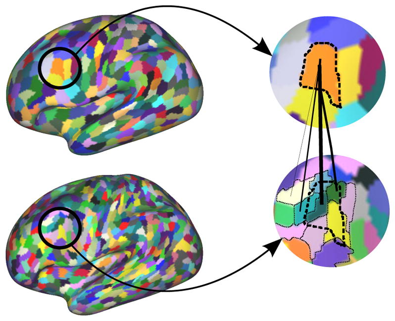
Illustration of the inter-resolutions links. Connections links are constructed between two supervertices at the different resolutions if they share vertices on the original mesh. The strength of the edge is established by the number of shared vertices.
These links allow simultaneous clustering of the three base parcellation levels into a coherent K clusters parcellation represented at different levels of precision (based on the size of the supervertices). This is done following the multi-scale normalised cut method (Yu and Shi, 2003). In this setting, we seek to recover for each scale s a N × K parcellation matrix that describes the cluster assignments of the supervertices:
| (3) |
All resolutions can then be parcellated simultaneously by concatenating all parcellation and affinity matrices into global multi-scale parcellation and affinity matrices:
| (4) |
Here Wi is the merged affinity matrix associated with the resolution level i. Coherence of the parcellations between the different resolutions is enforced by the inter-resolution links that are encoded in the following constraint matrix:
| (5) |
Here IN is the N × N identity matrix.
This matrix controls the obtained parcellation over all scales through an imposed constraint on the parcellation matrix:
| (6) |
Spectral decomposition of the multi-scale affinity matrix WSi subject to equation 6 yields a parcellation that captures variations in connectivity profiles at different scales. At each resolution, the supervertices are assigned to a particular parcel. This results in parcellations at different degrees of precisions in terms of boundaries, depending on the supervertex resolution.
A limitation of the proposed multi-scale parcellation is the absence of correspondences between subjects, which is essential if one is aiming to identify group specific connectivity features. Parcel boundaries can substantially vary across subjects, due to noise and anatomical differences. Group-wise parcellation can provide parcellations that are more robust with respect to locally unreliable data on the subject level, while at the same time ensuring that correspondences are enforced across subjects.
2.5. Group-wise Parcellation
It is straightforward to rewrite the N models (one per subject) into a joint optimisation problem. This can be done very easily by concatenating all the subjects’ affinity and inter-scale constraint matrices, which results in the estimation of a joint parcellation matrix defined as follows:
| (7) |
while the joint affinity and constraint matrix can be defined as:
| (8) |
In this setting however, all the subjects’ parcellations are estimated independently and no correspondences are enforced. Obtaining a meaningful matching parcellation across subjects requires the definition of inter-subject connections that describe which regions should be assigned to the same label.
For this task, we cannot solely rely on the cortical surface registration for two reasons. First, anatomical/sulcal alignment does not imply that structural connections are registered as well, i.e. connectivity patterns can differ locally across subjects. The same parcellation should not be imposed on subjects who have different local connectivity profiles. Second, the registration itself is likely imperfect, and local errors could affect the structural correspondences between subjects. For those reasons, direct vertex to vertex comparisons across subjects are not reliable enough to obtain meaningful matches. Carrying comparisons on the supervertex scale (Parisot et al., 2015) can decrease the impact of a poor alignment. However, the connections remain subpar and biased with anatomical information since our data is only aligned in terms of cortical folding. These possible errors and biases are likely to get stronger if we increase the resolution of our supervertex parcellations as we get closer to a vertex to vertex comparison set up.
We are tackling these issues with a two-fold approach. When seeking to match a supervertex in subject Si (supervertex belonging to the coarsest resolution) with a supervertex in another subject Sj, we first follow the approach in Parisot et al. (2015) and find the supervertex that has the highest overlap (in terms of number of original mesh vertices) with . We then consider all the supervertices that are immediate neighbours of and seek the one with the most similar connectivity pattern with the rest of the brain. As connectivity profiles can differ from one brain to the next, we do not directly compare the connections across the brain, but the correlation of connectivity profiles of one supervertex with all the others. In other words, we compare if two supervertices are similar in terms of connectivity to the same cortical regions, even though the actual connectivity profiles of these supervertices can differ.
Inter-subject edges are created between the matched supervertices and and weighted as the correlation between the low dimensional merged connectivity profiles associated with each supervertex:
| (9) |
Here α is a weighting parameter that controls the influence of the inter-subjects weights and ρ(.) is the Pearson’s correlation coefficient. Weighting the edges with the correlation between the matched supervertices allows control of how similar two parcellations are expected to be locally, based on the similarity of the two subjects’ underlying data.
The inter-subject anatomical and connectivity variability is further accounted for by limiting the connection between subjects to the coarsest supervertex parcellation resolution. This allows more differences between parcellations at the higher resolution (i.e. parcellations that are more faithful to the subject’s connectivity information) while at the same time ensuring correspondences between the parcellations.
The inter-subject edges are incorporated in the framework by updating the group-wise affinity matrix (Eq. 8) as follows:
| (10) |
2.6. Optimisation
The next step is the joint spectral decomposition of this affinity matrix subject to the inter-layer constraints to recover the group’s parcellation matrix. The group-wise parcellation can be recovered by optimising the following multi-scale normalised cut objective criterion:
| (11) |
| (12) |
| (13) |
| (14) |
This problem is unfortunately NP-complete, but a near global-optimal solution can be estimated in a two-step approach (Cour et al., 2005). The first step is to solve the relaxed continuous problem Z* derived from problem 11. This is done using the Rayleigh-Ritz theorem (Yu and Shi, 2004) by computation and normalisation of the K largest eigenvector of a matrix QPQ, defined as:
| (15) |
Matrix P is the normalised affinity matrix obtained by multiplication with the degree matrix D of W. Q is the so-called projector matrix, that ensures we are seeking a solution that respects constraint 14.
The second optimisation step consists of discretising the global solution of Z* (Yu and Shi, 2003) so as to find the closest solution to the relaxed problem that satisfies the discrete problem.
The group average parcellation can then be obtained from the individual subjects parcellation through majority voting. Our objective using the simple majority voting approach is to identify which brain regions are in agreement between subjects, i.e. to find the regions that best summarise the similarities between subjects.
2.7. Evaluation: Quantitative Measures
The evaluation of brain parcellation tasks is a challenge in itself since there is no ground truth to compare to. In order to provide a quantitative evaluation of our approach, we compute measures that intuitively should be characteristic of a good parcellation.
2.7.1. Information Loss
Our first objective is to obtain parcellations that represent the data as well as possible. A parcel’s average connectivity profile should be as close as possible to all the connectivity profiles of the vertices within the parcel. We evaluate the faithfulness of our parcellations to the data by evaluating the information that is lost by approximating the vertices’ connectivity profiles with the parcels’ averages. This is done by creating a Nv × Nv matrix χav from the merged connectivity matrix, by assigning the same merged profile to all vertices in the same parcel (see Fig. 5). We then compute the Kullback-Leibler Divergence (KLD) between this matrix and the original tractography matrix χ that are normalised to be probability mass functions. The KLD measures how much information is lost by approximating the tractography matrix χ with χav. A low KLD therefore corresponds to a faithful parcellation.
Figure 5.

Illustration of the merging process in order to build a merged connectivity matrix and the Nv × Nv matrix.
2.7.2. Silhouette Index
We further evaluate the quality of our clustering using the Silhouette index (Rousseeuw, 1987), which is a commonly used cluster validity measure. It has notably been used several times for evaluation of brain parcellations (Craddock et al., 2012; Eickhoff et al., 2014). The Silhouette index computes for each vertex a score of confidence with respect to its cluster assignment.
| (16) |
Here a(v) is the average dissimilarity between v and all vertices within the same parcel. b(v) is the average dissimilarity between v and all elements in the cluster that has the highest similarity. The Silhouette index takes values between −1 and 1, where −1 suggests that the vertex has been misclassified. A value close to zero suggest that the vertex is equally similar to two different clusters. Here, we define the dissimilarity between vertices as the opposite of the correlation matrix.
2.7.3. Group Consistency
We evaluate the quality of our group-wise constraint through a group consistency measure that is inspired by the Minimum Description Length principle (Rissanen, 1978). After a group parcellation, we compute an average connectivity matrix by averaging all subjects’ merged connectivity matrices. The group average is then compared to each individual subject’s connectivity matrix, the idea being that the distance should be minimal if the average is representative of all subjects. The measure we compute is the Sum of Absolute Differences (SAD) between the normalised connectivity matrices. Normalisation allows fair comparisons across varying numbers of parcels. In addition, this measure has the potential to identify outliers within a group that will strongly differ from the group average.
2.7.4. Overlap Between Parcellations
Parcels are quantitatively compared and matched using the measure of spatial overlap proposed in Bohland et al. (2009). This measure is non symmetric, and evaluates the proportion of one region i that is contained in another region j. We refer to ri and rj as the ensembles describing the vertices that belong to regions i and j respectively. The similarity measure Pij is then defined as:
| (17) |
where |r| is the number of voxels in ensemble r. When applied on different subjects, this measure relies on the vertex correspondences obtained from the sulcal registration. A symmetric measure is also defined as .
We match two parcellations by selecting the parcels that have the highest similarity scores. It should be noted that several parcels can be matched to the same one and therefore merged into a larger parcel. We use the symmetric measure O as a measure of overlap for quantitative evaluation. This is more flexible than the commonly used Dice Similarity Coefficient as it does not search for perfect overlap but also for inclusion of a parcel in another. Furthermore, this approach allows to compare parcellations with a very different number of parcels, which can be very useful when comparing to other methods and modalities.
2.7.5. Bayesian Information Criterion
The proposed measurements used to evaluate single subject parcellations cannot be used for comparing group parcellations since our group-wise parcellation is not directly derived from a joint connectivity matrix. We compute instead the Bayesian Information Criterion (BIC) as described in Thirion et al. (2014) for evaluating group-wise parcellations.
We evaluate how well the parcellations agree with the underlying brain structure by comparing to task fMRI activation maps. Each vertex is associated with the concatenated task activation maps of all subjects within the group considered. The signal y(concatenated activation maps) within each parcel is modelled using a probabilistic model as:
| (18) |
Here, μ is the average signal within a parcel, X is a known matrix that identify which subject the vertex value corresponds to. The estimation of the parameters (μ, σ1, σ2) is carried out in each parcel using the Expectation Maximisation algorithm. Parameters σ1 and σ2 respectively express the variance within and between subjects. The BIC criterion then evaluates the goodness of fit by penalising the negative log likelihood by the complexity of the model (number of parcels).
3. Results
3.1. Parameter Selection
The parameter μ for the construction of the supervertices is set heuristically to 3. The parameter α that control the strength of the connections between the subjects has a more important impact on the obtained parcellation. α should be high enough to impose consistency between subjects but also allow local differences between them to remain faithful to the underlying data. Furthermore, isolated supervertices tend to appear when α is too high.
We make use of the KLD and SAD measures to optimise the parameters as they provide complementary information. We compute the KLD to make sure the parcellation remains faithful to the data, while the SAD evaluates if group consistency is imposed. We optimise α on one group of 50 subjects for both hemispheres. We compute the KLD and SAD for 20 to 250 parcels and α ranging from 0.01 to 3.5.
The first observation is that the measures follow what is expected intuitively with respect to the number of parcels: the KLD decreases with the number of parcels. This is expected since a high resolution reduces the amount of averaging necessary during the construction of the merged matrix. In contrast, the SAD progressively increases with the number of parcels. This is due to the fact that more anatomical differences are conserved when the resolution increases.
As shown in Fig. 6, both measures follow similar trends, sharply decreasing when increasing α, then stabilising or slowly increasing. The strong improvement of the measures at low α values can be explained by the fact that parcellations are not imposed to be similar if the connections are too weak, as a result, the number of parcels selected is spread across all subjects, resulting in very low parcellation resolutions for all subjects. This increases the value of the KLD (low resolution) and the value of the SAD (no agreement imposed between subjects).
Figure 6.

Evolution of the KLD (a) and SAD (b) value of α for the right hemisphere.
The SAD measure has a tendency to increase after reaching a minimum. Isolated supervertices tend to appear when the correspondences between subjects are set too high, which decreases the quality of the parcellation. We essentially seek parcellations that are faithful to the underlying connectivity data while preventing the appearance of isolated supervertices. Therefore, we select for each parcellation resolution the optimal value of α as the closest value that both stabilises the KL divergence and minimises the SAD. We observe for both hemispheres that the value of α has to be increased regularly with the number of parcels (Fig. 7).
Figure 7.
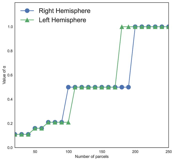
Evolution of the optimal value of α for both hemispheres.
All our remaining experiments are carried out on our second group of 50 subjects that have not used for parameter optimisation with the optimal value of α.
3.2. Methods comparison
After parameter optimisation, we perform the group-wise parcellation scheme on our second group. The first observation, as shown in Fig. 8, is that we obtain parcellations that have direct correspondences yet remain subject specific (i.e. the shape and location of parcels can differ from one subject to the next). Isolated supervertices may appear, which can be due to links that are too strong or too numerous.
Figure 8.

Visual example of single subject parcellations obtained from the group-wise scheme (100 parcels). Identical colours between different subjects indicate corresponding parcels (there is no inter-hemispheric matching).
The proposed group-wise method was then quantitatively compared to gyral (Destrieux et al., 2010) and random (Poisson disk sampling) parcellations, as well as connectivity driven parcellations from k-means, hierarchical and spectral clustering (Sec. 2.4 and normalised cuts (Craddock et al., 2012)). Hierarchical clustering is performed using the spatially constrained linkage method as described in Moreno-Dominguez et al. (2014). We are using the average linkage method as we have observed that it yields the best quantitative results. This has also been observed by Moreno-Dominguez et al. (2014) for dMRI driven parcellation. All clustering methods are initialised from the finest supervertex resolution so as to reduce the impact of noise. Hierarchical and spectral clustering methods are spatially constrained (we only preserve neighbouring connections) to obtain contiguous parcels. The spatial contiguity of k-means clusterings is artificially enforced by only keeping the connections with the 10 closest neighbours. This yielded compact parcels of similar sizes. Poisson Disk Sampling generates regions of approximately equal size by ensuring that two region centres are not closer than a given threshold which controls the number of obtained parcels. For single subject parcellations, correspondences between the different parcellations have to be established to compute the SAD. The matching is suboptimal since boundaries can be very different across subjects. This biases the values of the SAD but also highlights the main issue associated with single-subject parcellations which is the difficulty to find correspondences between subjects.
We compute the KLD, SAD and Silhouette index for all methods. Figure 9 shows boxplots of the measures for all methods and subjects in the group. We observe that spectral methods tend to show better performance for all measurements and that the group-wise approach yields very similar KL values as the single subject approach. In other words, the obtained parcellations remain as faithful to the data despite the group constraint while achieving the best results in terms of group consistency. The same behaviour can be observed for Silhouette index computations.
Figure 9.

Boxplots of the values of the KLD (a), SAD (b) and Silhouette index (c) for all parcellation methods.
Interestingly, k-means clustering yields the best performance for KLD measurements, but the lowest score amongst connectivity driven methods for both Silhouette index and SAD. On the one hand, the different spatial constraint (keeping the 10 closest neighbours rather than the nearest neighbour) could allow to construct parcellations that follow connectivity patterns more precisely. On the other hand, this limited constraint yields irregular clusters that are sensitive to noise, which reduces the quality of the parcellation and its reproducibility. This assumption is supported by the low performances obtained for the Silhouette index and SAD (quality of clustering and group consistency). Furthermore, we also observe an increase in performance for all measurements using our multi-scale approach compared to Normalised cuts. This highlights the added value of using multiple scales for the parcellation task. The gap in performance is particularly striking for Silhouette index computations.
Since the surfaces have been registered based on sulcal information, we expect strong similarities between subjects regarding the gyral parcellation. This is confirmed by the low values of the SAD, which are on par with the ones obtained from the group-wise parcellation. The performance in terms of information loss and cluster validity indices is on the other hand the worst across all methods.
3.3. Inter-modality Comparisons
We then compared the boundaries of our parcellations with myelin maps, Brodmann’s areas and fMRI task activation maps. All modalities are obtained from the HCP dataset (myelin, Brodmann) Glasser et al. (2013) or using the HCP processing scripts (task fMRI). Myelin maps are calculated as the ratio of T1-weighted and T2-weighted MRI (Glasser and Van Essen, 2011). The Brodmann parcellation was mapped onto the Conte69 brain surface atlas (Van Essen et al., 2012). It was then mapped onto each subject’s surface using the cortical folding driven registration’s deformation field.
The task fMRI data is preprocessed following the HCP preprocessing pipelines (gradient unwarping, motion and distortion correction, registration to the MNI space and projection to the cortical surface). Task activation maps are then obtained using standard FSL tools (FEAT) that use general linear modelling to construct activation maps (Barch et al., 2013). The analysis is carried out across sessions (single subject activation maps) and then across subjects (group-wise activation map).
Observations are made on the group average level, as well as the individual subject level. Our aim is to show that we obtain sensible average maps as well as faithful individual maps. All modalities provide complementary information, and therefore a complete match cannot be expected in any of the cases. However, we can expect local correlation between our parcel boundaries and other modalities.
For all resolutions, we observe strong correspondences between our parcels’ boundaries and strong variations of myelination, specifically in the motor areas, both on the average map and the single subject level. This is illustrated in Fig. 11 for randomly selected subjects and the average maps.
Figure 11.

Visual examples of the overlap between our parcels’ boundaries (black lines) and Brodmann areas (a,b), myelin maps (d–f), the composite parcellation Van Essen et al. (2012) (c) for two randomly selected subjects and the group average map.
Furthermore, single subject parcellations appear to have similar boundaries with Brodmann’s cytoarchitectonic motor areas (BA 1, 2, 3a–b, 4a–b and 6). Quantitative comparisons are proposed on the basis of the atlas concordance measure of Bohland et al. (2009). For all parcellation resolutions, we compute the overlap O between all Brodmann areas and our parcels. Due to the small size of these regions, areas BA 1, 3 and 4 are merged into a single parcel. We compare the quantitative results obtained with the other considered parcellation methods (spectral, hierarchical and random). In particular, random parcellations show how our results relate to chance. Figure 10 shows boxplots of the average overlap scores over all subjects for all resolutions, Fig. 11 shows visual examples of the overlap for different subjects, while Fig. 12 shows a spatial comparison to random parcellations overlap scores. On average over all parcellation resolutions, we obtain very good overlap measurements with the motor areas (BA 1–6), and outperform other methods. Interestingly, we observe that good overlap scores are only obtained around the motor area for all connectivity driven methods. The fact that results can be significantly lower than the overlap with random parcellations for all subjects and methods in some areas could suggest that either the structural connectivity differs with cytoarchitecture, or that the Brodmann map and structural connectivity data are not properly registered.
Figure 10.

Boxplots of the average overlap over all subjects between our parcels and Brodmann areas for all computed resolutions. (a) left hemisphere, (b) right hemisphere.
Figure 12.

Comparison of the performance of the group-wise parcellation w.r.t random parcellations for (a) the Brodmann map and (b) the composite parcellation Van Essen et al. (2012). Values higher than zero (red to yellow) have a higher overlap than random parcellations, worse overlaps are shown in blue. (a) For each parcel, we count the number of times a parcel overlaps better (+1) or worse (−1) for all subjects and parcellation resolutions. (b) Overlaps are compared for 200 parcels, and averaged over the 50 random parcellations. Yellow and cyan parcels have an overlap difference of more than 20 % between both parcellations, other cases are shown in red and blue.
Our average parcellation is also compared to the composite parcellation proposed in Van Essen et al. (2012) where each region is derived from reliable local parcellations. Parcels are derived from different modalities such as cytoarchitecture and rhetinotopy. Given the size of most regions, we compare the parcellation to a high resolution connectivity driven parcellation (200 regions). Visual comparisons are shown in Fig. 11c and comparisons with the performance of random parcellations are shown in Fig. 12b. Here again, we compute overlap scores between our group average and the composite parcellation and compare it to the performance of random parcellations. We again obtain good performance around the motor area, and worse results in other regions, notably around the visual cortex. In addition to data quality and disagreement of dMRI with other modalities, these results could be linked to the size of the groups used to build the composite and group parcellations, which could be too small to fully correspond. Another explanation could be that some regions have too much inter-subject variability and cannot be summarised properly without a dMRI driven registration step.
Task activations are only compared on the group level due to the fact that individual task activation maps can be very noisy. We are therefore only comparing our average parcellation to average activation maps. Visual comparisons are proposed in Fig. 13 between the boundary of our average parcellations and activation maps for different tasks.
Figure 13.

Visual examples of the correspondences between average task activation maps and our average parcels’ boundaries for a group of 50 subjects.
3.4. Group-wise Parcellation Evaluation
While a set of 50 subjects remains limited, group parcellations at this level should start showing consistency across different groups and are less sensitive to inter-subject variability. We evaluate the reproducibility between two different groups by comparing our average parcellations obtained from our two groups of 50 subjects. The average parcellations are computed through majority voting from all 50 individual parcellations, while the average connectivity map is simply the average of all subjects’ merged connectivity maps.
We computed the overlap between our different parcels after matching them, as well as the SAD in order to compare the built connectivity networks. Those values are compared to the ones obtained between two independent single subject parcellations and the overlap between two subjects parcellated within the same group. The evolution of the overlap with respect to the number of clusters is shown in Fig. 14.
Figure 14.

Quantitative evaluation of the group consistency, compared to the intra-group consistency (obtained from a group-wise parcellation) and the inter-group consistency (obtained from single subject parcellations).
After matching the parcels, we also computed the SAD between the two average maps. As expected, the value tends to increase with the number of parcels and are lower than the intra group SAD scores. However, we consistently obtain better values than the one obtained between spectral individual parcellations (where the matching process is identical) and, as illustrated in Fig. 15, very similar connectivity maps at low resolutions. Figure 16 shows how reproducible two regions are within the same group on average over all resolutions. We observe a similarity between reproducible regions between the two hemispheres.
Figure 15.

Visualisation of the absolute difference between connectivity networks: (a, b) difference between the networks obtained for two subjects using single subject parcellation (a), and group-wise parcellation (b); (c) difference between the average networks for the two different groups tested. The circle represents the parcels on the cortical surface, connections are the edges connecting the parcels. The edges and their thickness correspond to the difference in connectivity strength (probtrackX fibre count) between the compared networks. The different colours are used here for visualisation purposes to differentiate the edges.
Figure 16.
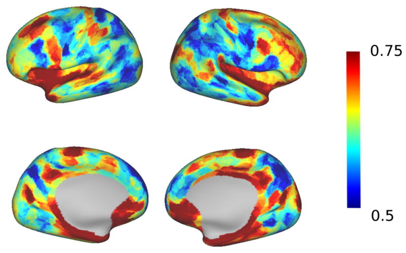
Local overlap between the two group averages, averaged over all resolutions.
Our group-wise parcellations from the second group (not used for parameter optimisation) are also quantitatively compared the group-wise parcellations obtained using common clustering methods (k-means, hierarchical (using the average linkage method) and spectral clustering (normalised cuts and our multi-scale approach)) on the average connectivity matrix. For all clustering tasks, the affinity matrix driving the clustering is the Pearson’s correlation co-efficient between the average connectivity profiles over all 50 subjects in the group. We do not compare to other group averages from single-subject methods here since the differences between single-subject parcellations are too high to construct a meaningful average map. Methods are compared quantitatively using the BIC criterion (sec. 2.7.5). The same task fMRI contrasts as the ones proposed in Thirion et al. (2014) are considered here: the faces-shape contrast of the emotional protocol, the punish-reward contrast of the gambling protocol, the math-story contrast of the language protocol, the left foot-average and left hand-average contrasts of the motor protocol, the match-relation contrast of the relational protocol, the theory of mind-random contrast of the social protocol and the two back-zero back contrast of the working memory protocol.
Results are shown in Fig. 17 for both hemispheres and all resolutions considered (20 to 250 parcels). We can see that the spectral methods yield the best results (lower values are better) for both hemispheres and most resolutions. Our group-wise approach tends to yield better results at the highest resolutions, which could be linked to the fact that the lack of registration between dMRI connectivity networks (which will impact the average connectivity matrix) has a stronger impact when more precision is required.
Figure 17.

Comparison of group-wise parcellation methods using Bayesian Information Criterion scores for both hemispheres. Lower values correspond to better scores.
We also visualise the average intra and inter-subjects variance parameters of the model (σ1 and σ2 respectively) in Fig. 18. All methods have similar behaviour: the intra-subject variance monotonously decreases with the number of parcels, while the inter-subject variance follows the opposite trend. A similar behaviour was observed in Thirion et al. (2014). All methods appear to have similar variances, with hierarchical and k-means clustering having the largest inter-subject variance and intra-subject variance respectively.
Figure 18.

Comparison of the intra and inter-subject model variance between group-wise parcellation methods both hemispheres.
4. Discussion
In this paper, we proposed a connectivity-driven parcellation method inspired from the concept of cosegmentation. The proposed method simultaneously estimates subject specific parcellations that have direct correspondences across subjects. Quantitative and qualitative experiments show that group consistency does not reduce the quality of the parcellation on the subject level. Furthermore, the comparison between two independent groups shows that we can obtain a good reproducibility despite a relatively small sample size.
Our comparisons with myelin maps, task fMRI and cytoarchitecture show that we obtain parcel boundaries that reflect other modalities, especially in the motor area where we observe strong similarities. Inter modality comparisons should however be considered carefully. First, all different modalities are obtained after a series of processing steps where several errors could be introduced (cortical folding based registration, volume to surface projection, segmentation...). Furthermore, it is still unclear how much these modalities interact and how similar they are expected to be. Therefore, complete agreement is not to be expected. In particular, we have observed that all dMRI driven parcellations we considered are generally performing worse than random parcellations in terms of overlap with Brodmann areas that are not in the motor area. There are several facts that can explain this phenomenon. The Brodmann maps are obtained from a single subject, then projected onto an atlas, which is then registered to the single subjects based on cortical folding. The registration process is based on sulcal depth, which focuses strongly on the motor area where the folding patterns are more consistent between subjects. The observation that dMRI driven parcellations are performing worse than chance suggests that Brodmann areas’ boundaries are not properly aligned with the dMRI data. This is very likely to be the case for subjects that have very different folding patterns with respect to the reference surface. The fact that our comparisons are favourable in the motor area supports this theory. Other possible explanations could be that dMRI locally disagrees with cytoarchitectural boundaries, or that the dMRI processing steps and noise have introduced some errors that do not allow to recover these boundaries.
More generally, several facts associated with dMRI driven parcellations should be kept in mind when looking at the interpretability of parcellations or aiming at comparing them with different modalities (rs-fMRI parcellations for instance). dMRI and tractography represent the current best way of representing the physical connections in the brain in vivo. Parcels can therefore naturally be biologically interpreted as regions that are directly connected to the brain in a similar way. Because of this, dMRI is expected to be more robust and interpretable for longitudinal (ageing or development) connectome analysis than resting-state fMRI for instance, whose biological interpretation is not as natural (Eickhoff et al., 2015).
Nevertheless, the connections inferred from dMRI processing and tractography have to be considered carefully and put in perspective. The connections are obtained from the indirect measurement of the diffusion of water molecules in the brain. Processing the data and inferring the tracts is a tremendous problem in itself, and many aspects remain problematic. Large fibre bundles are often predominant, while crossing and kissing fibres are often difficult to differentiate. Long range connection can also often be missed, due to a growing uncertainty along the tract. This makes tractography data prone to false negatives (interestingly, rs-fMRI is on the contrary prone to false positives). Another difficulty is to precisely determine the origin of the tracts, tractography having been observed to have a bias with ending tracts in gyri (Van Essen et al., 2013; Ng et al., 2013), this could notably affect the location of parcel boundaries and should be remembered when comparing parcellations to other modalities for instance. Despite these encountered difficulties, dMRI remains the best way of evaluating the physical tracts in vivo. While the obtained tracts could not be completely accurate, the evaluated similarity between connectivity profiles could still be correct (Knösche and Tittgemeyer, 2011), leading to accurate parcellations.
One drawback of spectral clustering approaches is the tendency to create similarly sized parcels. This size bias could explain why the quality of the correspondences with cytoarchitectonic regions and task activation maps varies from one resolution to the next. Indeed, it is possible that some transitions in connectivity can only be captured at specific resolutions or degrees of precision. This phenomenon could prevent from determining an optimal number of parcels as specific boundaries could be identified at specific resolutions. For this reason, the main objective of our evaluation was not to find an optimal number of parcels but rather to compare our approach at a given resolution with others. A possible way of exploiting this hierarchy of parcellations would be to combine the parcellations obtained at different resolutions, or identifying the most reliable boundaries over all resolutions. Another issue associated with the hierarchical and spectral clustering method considered here is the imposed spatial constraint to obtain spatially contiguous parcels: on the one hand, only connections between neighbouring vertices are kept, which can lose critical information. On the other hand, parcel can be subject to noise and irregular, as observed with k-means clustering results.
One of the main advantages of using a group-wise parcellation method is the possibility to perform direct comparisons between subjects as well as groups (gender, age or diseased base groups). At the single subject level, this allows to estimate which brain regions are the most consistent (inter-subject variability), while the group level enables to evaluate the fundamental differences in connectivity and function between two different groups. This could provide information about the impact of a disease on the brain for instance. One big challenge would be to identify whether the differences are due to noise and processing errors or actual biological differences. Comparing one subject to the group could be a way of identifying if a region in a specific subject is governed by noise. Our method reduces the influence of noise and registration errors by finding local correspondences at a coarse supervertex parcellation level and carrying a neighbourhood search. This setting is better suited for identification of similarities between subjects when working at the subject level. Group differences can then be considered as noise should be strongly reduced at the group level.
A natural extension of the method would be to run it on much larger groups in order to evaluate the reproducibility and obtain parcellations that are truly independent from inter-subject variability. Consequently we could estimate more reliably the global differences between different kinds of groups. A further exploration of the parameter space on a larger group would also allow a better design of the inter-subject edges. Finally, inter-modality comparisons could be performed by applying the method to resting state fMRI. Comparing or combining dMRI and rs-fMRI driven parcellations could enable to identify functionally specialised regions more accurately than by using a single modality.
Acknowledgments
The research leading to these results has received funding from NIH grant P41EB015902 and the European Research Council under the European Union’s Seventh Framework Programme (FP/2007–2013)/ERC Grant Agreement no. 319456. Data were provided by the Human Connectome Project, WU-Minn Consortium (Principal Investigators: David Van Essen and Kamil Ugurbil; 1U54MH091657) funded by the 16 NIH Institutes and Centers that support the NIH Blueprint for Neuroscience Research; and by the McDonnell Center for Systems Neuroscience at Washington University.
Footnotes
Human Connectome Project Database, https://db.humanconnectome.org/
References
- Achanta R, Shaji A, Smith K, Lucchi A, Fua P, Susstrunk S. Slic superpixels compared to state-of-the-art superpixel methods. IEEE T Pattern Anal. 2012;34:2274–2282. doi: 10.1109/TPAMI.2012.120. [DOI] [PubMed] [Google Scholar]
- Anwander A, Tittgemeyer M, von Cramon DY, Friederici AD, Knösche TR. Connectivity-based parcellation of Broca’s area. Cereb Cortex. 2007;17:816–825. doi: 10.1093/cercor/bhk034. [DOI] [PubMed] [Google Scholar]
- Arslan S, Parisot S, Rueckert D. Joint spectral decomposition for the parcellation of the human cerebral cortex using resting-state fmri. IPMI. 2015:85–97. doi: 10.1007/978-3-319-19992-4_7. [DOI] [PubMed] [Google Scholar]
- Barch DM, Burgess GC, Harms MP, Petersen SE, Schlaggar BL, Corbetta M, Glasser MF, Curtiss S, Dixit S, Feldt C, Nolan D, Bryant E, Hartley T, Footer O, Bjork JM, Poldrack R, Smith S, Johansen-Berg H, Snyder AZ, Essen DCV. Function in the human connectome: Task-fmri and individual differences in behavior. NeuroImage. 2013;80:169– 189. doi: 10.1016/j.neuroimage.2013.05.033. Mapping the Connectome. [DOI] [PMC free article] [PubMed] [Google Scholar]
- Behrens T, Berg HJ, Jbabdi S, Rushworth M, Woolrich M. Probabilistic diffusion tractography with multiple fibre orientations: What can we gain? NeuroImage. 2007;34:144–155. doi: 10.1016/j.neuroimage.2006.09.018. [DOI] [PMC free article] [PubMed] [Google Scholar]
- Blumensath T, Jbabdi S, Glasser MF, Van Essen DC, Ugurbil K, Behrens TE, Smith SM. Spatially constrained hierarchical parcellation of the brain with resting-state fMRI. NeuroImage. 2013;76:313–324. doi: 10.1016/j.neuroimage.2013.03.024. [DOI] [PMC free article] [PubMed] [Google Scholar]
- Bohland JW, Bokil H, Allen CB, Mitra PP. The brain atlas concordance problem: quantitative comparison of anatomical parcellations. PLoS One. 2009;4:e7200. doi: 10.1371/journal.pone.0007200. [DOI] [PMC free article] [PubMed] [Google Scholar]
- Brodmann K, Garey LJ. Brodmann’s: Localisation in the Cerebral Cortex. Springer Science & Business Media; 2007. [Google Scholar]
- Clarkson MJ, Malone IB, Modat M, Leung KK, Ryan NS, Alexander DC, Fox NC, Ourselin S. A framework for using diffusion weighted imaging to improve cortical parcellation. MICCAI. 2010;(1):534–541. doi: 10.1007/978-3-642-15705-9_65. [DOI] [PubMed] [Google Scholar]
- Cohen AL, Fair DA, Dosenbach NU, Miezin FM, Dierker D, Van Essen DC, Schlaggar BL, Petersen SE. Defining functional areas in individual human brains using resting functional connectivity mri. Neuroimage. 2008;41:45–57. doi: 10.1016/j.neuroimage.2008.01.066. [DOI] [PMC free article] [PubMed] [Google Scholar]
- Cour T, Bénézit F, Shi J. Spectral Segmentation with Multiscale Graph Decomposition. CVPR. 2005;(2):1124–1131. [Google Scholar]
- Craddock RC, James GA, Holtzheimer PE, Hu XP, Mayberg HS. A whole brain fMRI atlas generated via spatially constrained spectral clustering. Hum brain Mapp. 2012;33:1914–1928. doi: 10.1002/hbm.21333. [DOI] [PMC free article] [PubMed] [Google Scholar]
- Destrieux C, Fischl B, Dale A, Halgren E. Automatic parcellation of human cortical gyri and sulci using standard anatomical nomenclature. NeuroImage. 2010;53:1–15. doi: 10.1016/j.neuroimage.2010.06.010. [DOI] [PMC free article] [PubMed] [Google Scholar]
- Eickhoff SB, Laird AR, Fox PT, Bzdok D, Hensel L. Functional segregation of the human dorsomedial prefrontal cortex. Cerebral cortex. 2014:bhu250. doi: 10.1093/cercor/bhu250. [DOI] [PMC free article] [PubMed] [Google Scholar]
- Eickhoff SB, Thirion B, Varoquaux G, Bzdok D. Connectivity-based parcellation: Critique and implications. Human Brain Mapping. 2015;36:4771–4792. doi: 10.1002/hbm.22933. [DOI] [PMC free article] [PubMed] [Google Scholar]
- Girard G, Whittingstall K, Deriche R, Descoteaux M. Towards quantitative connectivity analysis: reducing tractography biases. Neuroimage. 2014;98:266–278. doi: 10.1016/j.neuroimage.2014.04.074. [DOI] [PubMed] [Google Scholar]
- Glasser MF, Sotiropoulos SN, Wilson JA, Coalson TS, Fischl B, Andersson JL, Xu J, Jbabdi S, Webster M, Polimeni JR, Essen DCV, Jenkinson M. The minimal preprocessing pipelines for the Human Connectome Project. NeuroImage. 2013;80:105– 124. doi: 10.1016/j.neuroimage.2013.04.127. [DOI] [PMC free article] [PubMed] [Google Scholar]
- Glasser MF, Van Essen DC. Mapping human cortical areas in vivo based on myelin content as revealed by t1-and t2-weighted mri. The Journal of Neuroscience. 2011;31:11597–11616. doi: 10.1523/JNEUROSCI.2180-11.2011. [DOI] [PMC free article] [PubMed] [Google Scholar]
- Honnorat N, Eavani H, Satterthwaite T, Gur R, Gur R, Davatzikos C. GraSP: Geodesic Graph-based Segmentation with Shape Priors for the functional parcellation of the cortex. NeuroImage. 2015;106:207–221. doi: 10.1016/j.neuroimage.2014.11.008. [DOI] [PMC free article] [PubMed] [Google Scholar]
- Jbabdi S, Sotiropoulos SN, Savio AM, Graña M, Behrens TEJ. Model-based analysis of multishell diffusion MR data for tractography: How to get over fitting problems. Magn Reson Med. 2012;68:1846–1855. doi: 10.1002/mrm.24204. [DOI] [PMC free article] [PubMed] [Google Scholar]
- Jbabdi S, Woolrich MW, Behrens TE. Multiple-subjects connectivity-based parcellation using hierarchical Dirichlet process mixture models. NeuroImage. 2009;44:373–384. doi: 10.1016/j.neuroimage.2008.08.044. [DOI] [PubMed] [Google Scholar]
- Johansen-Berg H, Behrens T, Robson M, Drobnjak I, Rushworth M, Brady J, Smith S, Higham D, Matthews P. Changes in connectivity profiles define functionally distinct regions in human medial frontal cortex. Proceedings of the National Academy of Sciences of the United States of America. 2004;101:13335–13340. doi: 10.1073/pnas.0403743101. [DOI] [PMC free article] [PubMed] [Google Scholar]
- Kim E, Li H, Huang X. CVPR. IEEE; 2012. A hierarchical image clustering cosegmentation framework; pp. 686–693. [Google Scholar]
- Knösche TR, Tittgemeyer M. The role of long-range connectivity for the characterization of the functional-anatomical organization of the cortex. Frontiers in Systems Neuroscience. 2011:5. doi: 10.3389/fnsys.2011.00058. [DOI] [PMC free article] [PubMed] [Google Scholar]
- Lashkari D, Vul E, Kanwisher N, Golland P. Discovering structure in the space of fmri selectivity profiles. Neuroimage. 2010;50:1085–1098. doi: 10.1016/j.neuroimage.2009.12.106. [DOI] [PMC free article] [PubMed] [Google Scholar]
- Mars RB, Jbabdi S, Sallet J, O’Reilly JX, Croxson PL, Olivier E, Noonan MP, Bergmann C, Mitchell AS, Baxter MG, et al. Diffusion-weighted imaging tractography-based parcellation of the human parietal cortex and comparison with human and macaque resting-state functional connectivity. The Journal of Neuroscience. 2011;31:4087–4100. doi: 10.1523/JNEUROSCI.5102-10.2011. [DOI] [PMC free article] [PubMed] [Google Scholar]
- Moreno-Dominguez D, Anwander A, Knösche TR. A hierarchical method for whole-brain connectivity-based parcellation. Hum Brain Mapp. 2014;35:5000–5025. doi: 10.1002/hbm.22528. [DOI] [PMC free article] [PubMed] [Google Scholar]
- Mota BD, Fritsch V, Varoquaux G, Banaschewski T, Barker GJ, Bokde AL, Bromberg U, Conrod P, Gallinat J, Garavan H, Martinot JL, Nees F, Paus T, Pausova Z, Rietschel M, Smolka MN, Ströhle A, Frouin V, Poline JB, Thirion B. Randomized parcellation based inference. NeuroImage. 2014;89:203– 215. doi: 10.1016/j.neuroimage.2013.11.012. [DOI] [PubMed] [Google Scholar]
- Ng B, Varoquaux G, Poline J, Thirion B. Implications of inconsistencies between fmri and dmri on multimodal connectivity estimation. In: Mori K, Sakuma I, Sato Y, Barillot C, Navab N, editors. Medical Image Computing and Computer-Assisted Intervention – MICCAI 2013. Springer; Berlin Heidelberg: 2013. pp. 652–659. volume 8151 of Lecture Notes in Computer Science. [DOI] [PubMed] [Google Scholar]
- Parisot S, Arslan S, Passerat-Palmbach J, Wells WM, III, Rueckert D. Tractography-driven groupwise multi-scale parcellation of the cortex. IPMI. 2015 doi: 10.1007/978-3-319-19992-4_47. [DOI] [PMC free article] [PubMed] [Google Scholar]
- Passingham RE, Stephan KE, Kötter R. The anatomical basis of functional localization in the cortex. Nature Reviews Neuroscience. 2002;3:606–616. doi: 10.1038/nrn893. [DOI] [PubMed] [Google Scholar]
- Peyré G, Cohen LD. 3DPVT. IEEE Computer Society; 2004. Surface segmentation using geodesic centroidal tesselation; pp. 995–1002. [Google Scholar]
- Rissanen J. Modeling by shortest data description. Automatica. 1978;14:465–471. [Google Scholar]
- Robinson EC, Jbabdi S, Glasser MF, Andersson J, Burgess GC, Harms MP, Smith SM, Van Essen DC, Jenkinson M. MSM: A new flexible framework for Multimodal Surface Matching. Neuroimage. 2014;100:414–426. doi: 10.1016/j.neuroimage.2014.05.069. [DOI] [PMC free article] [PubMed] [Google Scholar]
- Roca P, Rivière D, Guevara P, Poupon C, Mangin JF. Tractography-based parcellation of the cortex using a spatially-informed dimension reduction of the connectivity matrix. MICCAI. 2009 doi: 10.1007/978-3-642-04268-3_115. [DOI] [PubMed] [Google Scholar]
- Roca P, Tucholka A, Rivière D, Guevara P, Poupon C, Mangin JF. Inter-subject connectivity-based parcellation of a patch of cerebral cortex. MICCAI. 2010 doi: 10.1007/978-3-642-15745-5_43. [DOI] [PubMed] [Google Scholar]
- Rousseeuw PJ. Silhouettes: A graphical aid to the interpretation and validation of cluster analysis. Journal of Computational and Applied Mathematics. 1987;20:53–65. doi: 10.1016/0377-0427(87)90125-7. [DOI] [Google Scholar]
- Ryali S, Chen T, Supekar K, Menon V. A parcellation scheme based on von mises-fisher distributions and markov random fields for segmenting brain regions using resting-state fmri. Neuroimage. 2013;65:83–96. doi: 10.1016/j.neuroimage.2012.09.067. [DOI] [PMC free article] [PubMed] [Google Scholar]
- Sethian JA. A fast marching level set method for monotonically advancing fronts. Proceedings of the National Academy of Sciences. 1996;93:1591–1595. doi: 10.1073/pnas.93.4.1591. [DOI] [PMC free article] [PubMed] [Google Scholar]
- Shen X, Tokoglu F, Papademetris X, Constable R. Groupwise whole-brain parcellation from resting-state fMRI data for network node identification. NeuroImage. 2013;82:403– 415. doi: 10.1016/j.neuroimage.2013.05.081. [DOI] [PMC free article] [PubMed] [Google Scholar]
- Sporns O. The human connectome: a complex network. Ann NY Acad Sci. 2011;1224:109–125. doi: 10.1111/j.1749-6632.2010.05888.x. [DOI] [PubMed] [Google Scholar]
- Thirion B, Varoquaux G, Dohmatob E, Poline JB. Which fmri clustering gives good brain parcellations? Frontiers in neuroscience. 2014;8:13. doi: 10.3389/fnins.2014.00167. [DOI] [PMC free article] [PubMed] [Google Scholar]
- Tzourio-Mazoyer N, Landeau B, Papathanassiou D, Crivello F, Etard O, Delcroix N, Mazoyer B, Joliot M. Automated anatomical labeling of activations in spm using a macroscopic anatomical parcellation of the mni mri single-subject brain. NeuroImage. 2002;15:273–289. doi: 10.1006/nimg.2001.0978. [DOI] [PubMed] [Google Scholar]
- Van Essen DC, Glasser MF, Dierker DL, Harwell J, Coalson T. Parcellations and hemispheric asymmetries of human cerebral cortex analyzed on surface-based atlases. Cerebral cortex. 2012;22:2241–2262. doi: 10.1093/cercor/bhr291. [DOI] [PMC free article] [PubMed] [Google Scholar]
- Van Essen DC, Jbabdi S, Sotiropoulos S, Chen C, Dikranian K, Coalson T, Harwell J, Behrens T, Glasser MF. Diffusion MRI, 2nd: From Quantitative Measurement to In vivo Neuroanatomy. Academic Press; San Diego: 2013. —mapping connections in humans and non-human primates: Aspirations and challenges for diffusion imaging. [Google Scholar]
- Yeo BT, Krienen FM, Sepulcre J, Sabuncu MR, Lashkari D, Hollinshead M, Roffman JL, Smoller JW, Zöllei L, Polimeni JR, et al. The organization of the human cerebral cortex estimated by intrinsic functional connectivity. Journal of neurophysiology. 2011;106:1125–1165. doi: 10.1152/jn.00338.2011. [DOI] [PMC free article] [PubMed] [Google Scholar]
- Yu SX, Shi J. ICCV. 2. IEEE; 2003. Multiclass spectral clustering. [Google Scholar]
- Yu SX, Shi J. Segmentation given partial grouping constraints. IEEE T Pattern Anal. 2004;26:173–183. doi: 10.1109/tpami.2004.1262179. [DOI] [PubMed] [Google Scholar]
- Zilles K, Amunts K. Centenary of brodmann’s map—conception and fate. Nature Reviews Neuroscience. 2010;11:139–145. doi: 10.1038/nrn2776. [DOI] [PubMed] [Google Scholar]