Cell-type specific optical recording of membrane voltage dynamics in freely moving mice

Abstract

Electrophysiological field potential dynamics are of fundamental interest in basic and clinical neuroscience, but how specific cell types shape these dynamics in the live brain is poorly understood. To empower mechanistic studies, we created an optical technique, TEMPO, that records the aggregate trans-membrane voltage dynamics of genetically specified neurons in freely behaving mice. TEMPO has >10-fold greater sensitivity than prior fiber-optic techniques and attains the noise minimum set by quantum mechanical photon shot noise. After validating TEMPO’s capacity to track established oscillations in the delta, theta and gamma frequency-bands, we compared the D1- and D2-dopamine-receptor-expressing striatal medium spiny neurons (MSNs), which are interspersed and electrically indistinguishable. Unexpectedly, MSN population dynamics exhibited two distinct coherent states that were commonly indiscernible in electrical recordings and involved synchronized hyperpolarizations across both MSN subtypes. Overall, TEMPO allows the deconstruction of normal and pathologic neurophysiological states into trans-membrane voltage activity patterns of specific cell types.

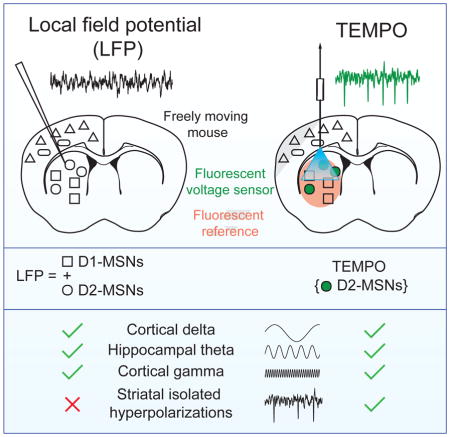
Graphical abstract

INTRODUCTION

Electrophysiological field potentials have drawn intense scrutiny since the early days of physiology (Adrian, 1928; Berger, 1929; Buzsaki et al., 2012; Steriade et al., 1993). Electroencephalographic (EEG) oscillations and event-related potentials indicate brain states that arise in specific forms of behavior, cognition and disease (Luck, 2014; Schnitzler and Gross, 2005; Uhlhaas and Singer, 2006). However, the cellular origins and mechanistic roles of field potential dynamics in brain function generally remain unclear (Kajikawa and Schroeder, 2011; Linden et al., 2011).

The biological challenges to dissecting these dynamics are at least twofold. First, field potentials typically reflect contributions from multiple cell types, some of which may be anatomically sparse. Second, they generally reflect a time-varying, unknown mixture of signal sources across multiple length scales, from local currents generated within ~100 μm to volume-conducted signals coming ~1 cm away from the recording probe (Buzsaki et al., 2012). This complexity has hindered biological interpretations of electric field oscillations, especially in areas that lack laminar structure and have multiple intermingled neuron types. Laminar brain areas allow charge source density analyses of the electrical sources in different laminae with different cell types, but such approaches are far less informative in non-laminar areas (Buzsaki et al., 2012; Mitzdorf, 1985).

Further, the extant means of recording cells’ trans-membrane voltages have not allowed studies of defined cell types in behaving animals. Intracellular electrode recordings are usually restricted to single cells, nearly prohibitive in behaving animals, and not easily targeted to specific cell types, especially in sub-cortical tissues. Genetically encoded Ca²⁺ indicators work well in behaving animals (Cui et al., 2013; Gunaydin et al., 2014; Ziv et al., 2013), but Ca²⁺ activity poorly reflects spiking activity in many cells, tracks neither subthreshold, inhibitory nor oscillatory activity well, and does not follow voltage waveforms on time scales finer than ~25–100 ms (Hamel et al., 2015).

By comparison, fluorescent indicators of trans-membrane voltage report subthreshold and inhibitory activity (Akemann et al., 2010; Gong et al., 2014; St-Pierre et al., 2014), and past studies used these indicators to monitor sensory evoked potentials in awake rodents, or voltage oscillations in anesthetized rodents (Akemann et al., 2012; Akemann et al., 2010; Carandini et al., 2015; Ferezou et al., 2006). However, genetically encoded voltage sensors have modest dynamic ranges, ~1% signal change per 10 mV voltage change in cultured cells and even less for signals averaged over a cell population.

These small signals are comparable to fluorescence fluctuations that arise in vivo from hemodynamics and brain motion (Akemann et al., 2012; Kalatsky and Stryker, 2003). Identification of optical voltage signals from identified cell populations has thus required averaging over multiple experimental trials, use of less-sensitive dual-color indicators, or illumination levels that cause rapid photobleaching and limit recordings from tens to hundreds of seconds (Akemann et al., 2012; Ferezou et al., 2006). To date no system for optical voltage recording has had the sensitivity to monitor identified cell types in freely behaving animals, nor to approach the physical sensitivity limits set by quantum mechanical photon shot noise (Hamel et al., 2015).

Here we report a fiber-optic method for recording the voltage dynamics of genetically specified cells in active mice. Unlike past approaches (Akemann et al., 2010; Ferezou et al., 2006), our system works well in superficial and deep brain areas. To stress that our method senses transmembrane and not extracellular voltages, we named it ‘Trans-membrane Electrical Measurements Performed Optically’ (TEMPO). TEMPO removes physiologically induced noise fluctuations, is ~10-fold more sensitive than fiber-optic methods for Ca²⁺ sensing (Gunaydin et al., 2014; Stroh et al., 2013), and approaches the photon shot noise sensitivity limit. This measurement sensitivity lowers the illumination needed, allowing recordings up to ~1 h long. We validated TEMPO by studying cortical and hippocampal oscillations in the delta, theta and gamma frequency bands in active mice.

To illustrate TEMPO’s utility in cell types poorly studied with field potential recordings, we examined D1- and D2-dopamine-receptor-expressing striatal medium spiny neurons (MSNs) in freely behaving mice. It is has been infeasible to distinguish these two MSN types based on their electrical activity or to isolate their contributions to the striatal local field potential (LFP). TEMPO revealed two distinct voltage waveforms, one a temporally isolated transient and the other a short-lived oscillation in both D1- and D2-MSNs, which were mutually synchronized during each of these. TEMPO also showed that MSNs hyperpolarize during these events and provided higher detection fidelity than electric field recordings, which generally did not reveal the isolated transients. Antagonism of D1- or D2-receptors evoked the two types of events to different extents, indicating direct links between dopamine signaling imbalances and abnormal levels of oscillation in striatal MSNs. TEMPO’s ability to connect specific cell types with macroscopic electrophysiological phenomena offers new means to dissect neurophysiologic states into their cellular constituents.

RESULTS

Measurement strategy

TEMPO has four key elements that jointly allow optical voltage sensing at the physical sensitivity limits while minimizing the impact of optical artifacts (Figure 1). First, to track concurrently neural voltage dynamics and physiologically induced artifacts, we co-expressed a green voltage sensor that undergoes approximately linear changes in fluorescence intensity as a function of trans-membrane voltage (MacQ-mCitrine or Ace2N-4AA-mNeon) (Gong et al., 2015; Gong et al., 2014), and a red reference fluor that we used to track optical fluctuations due to hemodynamics and brain motion (mCherry or tdTomato). This approach was based on studies in which we co-expressed static green and red fluors to assess the fluctuations alone. Despite the wavelength differences the red and green fluctuations correlated strongly (Figure S1), showing one can use the detected emissions of a red reference fluor to remove artifacts in recordings with a green voltage sensor.

Figure 1. Instrumentation for optical voltage tracking.

(A) Optical schematic. Two single-mode lasers emit 488 nm and 561 nm light. Photodiodes (PD) track the fluctuations in the beams’ intensities. The beams are combined in a dichroic mirror and focused into a polymer-clad multi-mode optical fiber, which delivers the light to the brain via an implanted fiber. Fluorescence returns via this fiber, is split into red and green emissions, and is detected by photoreceivers (PR).

(B) Phase-sensitive detection scheme. To shift the detection band away from low-frequency electronic noise, we applied sinusoidal amplitude modulation to both laser beams, at either 900 Hz or 3.5 kHz, depending on the detection bandwidth. Lock-in amplifiers (Lock-in), each phase-referenced to the modulation, tracked the intensities of both beams and emission channels. To distinguish emissions excited by the two beams, the two beams’ modulations were 90° out of phase, which was thus also apparent in the emissions.

(C) Signal generation and unmixing. The green and red fluorescence signals reflect a mixture of neural activity, brain motion and hemodynamic artifacts, and are respectively multiplied by the blue and green illumination intensities, which vary due to laser power fluctuations and the sinusoidal modulations. A blind-source separation algorithm removes physiological artifacts and laser intensity noise from the neural activity traces. See also Figures S1, S2 and Supplemental Appendix 1.

Second, to remove crosstalk arising from spectral overlap of the emissions, we sinusoidally modulated the intensities of the two excitation lasers (488 nm and 561 nm wavelengths); the modulations of the two beams were 90° out of phase but at the same frequency (either 0.9 or 3.5 kHz) (STAR METHODS). This allowed us to separate the signals excited by the two lasers via their distinct modulation signatures. We used four lock-in amplifiers, each phase-locked to the laser modulation, to amplify detected signals and track laser power fluctuations. This shifted the detection band away from low frequencies at which detectors usually have greater electronic noise and allowed near-uniform sensitivity across a 1–50 Hz recording bandwidth (Figure S2).

Third, to deliver two colors of illumination to the brain and collect the resulting fluorescence, we chose two single mode lasers and a multimode optical fiber with the aim of minimizing auto-fluorescence. The fiber core diameter matched that of the collimated beams, to minimize coupling of illumination into fiber-optic cladding modes. Light in the cladding leaks into the fiber-optic coating where it can excite substantial auto-fluorescence (Vo-Dinh, 2015), a well-known challenge for fluorescence sensing studies that can necessitate separate fibers for illumination and signal collection (Cui et al., 2013).

Fourth, to isolate voltage-dependent signals from physiological artifacts in the detected traces, we used a custom blind-source separation algorithm (Figures 1C, 2A; Supplemental Appendix 1). Prior attempts to unmix these in voltage-imaging studies with head-fixed rodents used a principal component analysis (PCA) (Akemann et al., 2012; Carandini et al., 2015). PCA was ineffective in our studies and did not isolate the signals (Figure S3). This is unsurprising, as PCA is not designed to separate independent signal sources. Instead, we developed a two-stage unmixing algorithm. Stage one estimates the time-dependent, cardiovascular pulsations in the red emission channel. Stage two uses independent component analysis (ICA), an established algorithm for source separation, to extract a decontaminated voltage trace (Figures 2A, S3).

Figure 2. Blind source separation allows near shot-noise-limited measurement sensitivity.

(A) Blind source separation procedure. Green, g(t), and red, r(t), fluorescence traces, and an estimate of hemodynamic noise, h(t), are inputs to an independent component analysis (ICA). ICA unmixes these into statistically independent components, Ŝ(t), a voltage trace, brain motion artifacts, Â(t), and hemodynamic artifacts, Ĥ(t).

(B) Power spectra of intensity fluctuations from an unmixed 1-min recording in a freely moving mouse co-expressing YFP and mCherry. Both traces showed broadband power increases during mouse movement and prominent hemodynamic artifacts (fundamental frequency ± FWHM: 12 ± 0.3 Hz; second harmonic: 24 ± 0.8 Hz). However, across the detection band the power spectrum of the unmixed trace approached the theoretical sensitivity limits set by shot noise, as calculated in B and D for a source of stationary mean intensity subject to the same frequency-dependent sensitivity of photodetection as the actual signals (Supplemental Appendix 2). The ratio of the s.d. of the unmixed trace to that expected from shot noise was 1.5–1.6.

(C) Comparison of the distributions of fluorescence fluctuations, ΔF/F, in the YFP and unmixed signal traces to those expected from shot noise in the unmixed trace, for the mouse in B (N>10⁴ time points). Unmixed signal traces from two YFP/mCherry mice had 20- and 10-fold reductions in noise power compared to raw YFP emissions. Shading denotes the s.e.m., computed based on counting errors, and is barely discernible.

(D) Power spectra of fluctuations of unmixed fluorescence traces from behaving mice expressing MacQ-mCitrine and tdTomato. Unmixing yielded significant 90 ± 4% (mean ± s.e.m.) declines in the peak power of hemodynamic noise (N=12 recordings from 4 mice; * denotes P=0.003, Wilcoxon signed-rank test).

See also Figure S3 and Supplemental Appendix 2.

TEMPO extracts voltage signals at the physical sensitivity limits

Exploratory studies in control mice expressing mCherry and yellow fluorescent protein (YFP) revealed low-frequency fluctuations (<10 Hz), likely due to motion- and breathing-induced artifacts, which we expected would corrupt both color channels similarly. There was also a noise peak (~12 Hz) from cardiac pulsations (Figure 2B) (Kalatsky and Stryker, 2003), which, due to the wavelength-dependence of light absorption by hemoglobin, we expected would impact the two channels differently. Indeed, YFP/mCherry recordings showed that a time-invariant unmixing approach generally did not reduce fluctuations to the minimum set by shot noise. This spurred us to use two-stage unmixing, to explicitly account for the differential effects of cardiovascular fluctuations on the red and green channels.

To evaluate how well this algorithm improved TEMPO’s sensitivity, we applied it to the YFP/mCherry datasets, and achieved a ~10-fold decline in the integrated spectral power of physiological artifacts compared to the raw YFP emissions trace (Figure 2B,C). The power spectrum of the unmixed trace was nearly flat across 0–50 Hz, showing unmixing reduced both cardiovascular and brain motion artifacts. The distribution of fluctuation amplitudes in the unmixed data approached that of a shot-noise limited recording (Figures 2C, S2), showing TEMPO was operating at the sensitivity limits. As with control mice, for mice expressing MacQ-mCitrine and mCherry our algorithm reduced the power of cardiac-induced noise by ~10-fold (Figure 2D). Overall, TEMPO has ~10-fold greater optical sensitivity than prior fiber-optic recording approaches not using a reference channel or unmixing scheme.

As the unmixed voltage trace has shot noise from both color channels, both the reference and indicator fluors play key roles in noise removal (Supplemental Appendices 1, 2). Thus, one should minimize shot noise in the reference channel by brightly expressing the red fluor. Notably, the bright red fluor tdTomato contributed lower-amplitude fluctuations to our unmixed traces than the dimmer fluor mCherry (mean ± s.e.m. power spectral density of shot noise in 6 tdTomato mice was −90 ± 2 dB vs. −81 ± 2 dB in 12 mCherry mice; P = 0.005; Wilcoxon rank-sum test).

TEMPO and field potential recordings are consistent in laminar tissue

As a validation, we verified that TEMPO can track voltage rhythms in laminar tissue, where field recordings have long been fruitful. We studied somatosensory cortex in mice anesthetized with ketamine-xylazine, which induces low-frequency cortical oscillations. We virally expressed mCherry and MacQ-mCitrine in pyramidal cells (cortical layers 5 and 6) and performed simultaneous TEMPO, EEG and LFP recordings, with the LFP electrode tip 50–150 μm from the tip of the fiber optic ferrule (Figure 3A,B). The EEG and TEMPO traces exhibited delta rhythms with a consistent phase offset (EEG frequency: 1.3 ± 0.1 Hz; TEMPO: 1.25 ± 0.15 Hz; mean offset between TEMPO and EEG rhythms: 1.4º ± 0.6º; mean ± s.e.m.; N=4 mice; Figure 3C,D). In EEG but not TEMPO traces, YFP/mCherry mice had similar rhythms as the MacQ-mCitrine/mCherry mice (Figure S1). Thus, the detection of oscillations by TEMPO required expression of the voltage indicator and was not merely due to physiologic artifacts or noise.

Figure 3. TEMPO reports voltage oscillations in anesthetized and alert mice.

(A) We virally expressed a green voltage sensor and a red reference fluor (AAV2/5-CaMK2a-MacQ-mCitrine; AAV2/5-CaMK2a-mCherry) in pyramidal cells in mouse infragranular somatosensory cortex. An overlying, implanted optical fiber delivered illumination and collected fluorescence.

(B) Green, red and merged dual-color fluorescence images of a coronal cortical section, and a magnified two-photon image of infragranular cells in the same section. Pyramidal cells throughout the cortex expressed mCherry. The voltage sensor was expressed in layers 5 and 6. Leftmost three scale bars: 100 μm. Right scale bar: 25 μm.

(C) EEG and TEMPO traces from cortical pyramidal cells in ketamine-xylazine (KX) anesthetized mice. The two time traces revealed low-frequency oscillations with similar waveforms.

(D) To assess the coherence of TEMPO and EEG oscillations, we computed the EEG–TEMPO cross-correlation in 4-s-increments across the 30-min session. It had a consistent peak amplitude and phase offset, showing the two traces had comparable dynamics over the session. We made similar findings as in B–D in N=4 mice.

(E) EEG and TEMPO signals from PV interneurons in mice under KX anesthesia. The two sets of time traces were often closely matched and revealed low-frequency oscillations. N=3 mice.

(F) Mean TEMPO and LFP traces relative to the transition of neurons from a hyperpolarized to a depolarized state in pyramidal cells and PV interneurons. Both cell types had similar, but significantly different temporal and phase offsets between the TEMPO and the LFP. (The polarity of the plotted LFP trace is the reverse of the EEG in C and E).

(G) An epi-fluorescence image of a coronal section from somatosensory cortex, and a two-photon image of cells in the same section reveal viral expression of a green voltage sensor (AAV2/9-CaMK2a-Ace2N-4AA-mNeon). The mouse (A2a-Cre × Ai14 tdTomato) expressed a red tdTomato reference fluor, which in cortex was largely confined to the vasculature. Similar expression in N=5 mice. Upper scale bar: 100 μm. Lower scale bar: 25 μm.

(H) TEMPO and LFP signals during bilateral tactile stimulation of the whiskers and ears. Upper, Mean TEMPO and LFP signals. Lower, Mean time courses of gamma-band (20–80 Hz) power. Both modalities showed a significant rise in gamma-band power during stimulation (P<10⁻¹⁰; Wilcoxon signed-rank test; N=389 stimulus trials in 5 mice). Shading denotes s.e.m. over trials.

(I) Single trial examples of gamma-band activity. Upper, Rises in gamma-band power typically occurred in 100–200 ms bursts, concurrent with depolarizations as seen in the TEMPO traces. Middle, Transient gamma-band bursts generally coincided in the two modalities. Lower, Time courses of gamma-band power were similar between the two modalities. See also Figure S4.

TEMPO can monitor sparse cell types

A key constraint of EEG and LFP recordings is the inability to selectively track anatomically sparse cell types. To show TEMPO has no such constraint, we studied cortical parvalbumin-positive (PV) interneurons, a relatively sparse class of inhibitory cells (Hu et al., 2014). We co-injected PV-Cre mice with AAV2/5-CAG-DIO-MacQ-mCitrine and AAV2/5-CaMK2a-mCherry. Fluorescent PV cells were in cortical layers 2/3–5/6, matching their known distribution (Figure S4). In anesthetized mice, 1–3 Hz delta rhythms arose in both the EEG and TEMPO traces (EEG frequency: 1.2 ± 0.04 Hz; TEMPO frequency in PV cells: 1.2 ± 0.1 Hz; mean ± s.e.m; N=3 mice) (Figure 3E).

We compared phase offsets between the delta rhythms in PV cells to those in pyramidal cells of layers 5 and 6. We aligned the TEMPO traces to moments of a switch from a hyperpolarized to a depolarized state, noting that emission declines from MacQ-mCitrine report depolarizations and rises report hyperpolarizations (Gong et al., 2014). At these transitions, LFP traces showed negative-going voltage spikes, but with distinct temporal offsets from the transitions seen by TEMPO in the two cell types (Figure 3F) [Mean ± s.e.m. offsets between LFP voltage minima and TEMPO zero-crossings: 23 ± 2 ms (pyramidal) vs. −4 ± 10 ms (PV); Phase offsets: 11º ± 1º (pyramidal) vs. −10º ± 7º (PV); both P < 10⁻⁵; Wilcoxon rank-sum test; N=2264 transitions (pyramidal; N=4 mice) vs. 128 (PV; N=3 mice)]. This fits with past reports of coordinated switching between hyperpolarization and depolarization in pyramidal cell and interneuron populations, but with a briefer delay to spiking upon depolarization in many interneurons (Massi et al., 2012).

TEMPO reports high-frequency rhythms in awake mice

To examine high-frequency rhythms, we studied pyramidal cells in somatosensory cortex of awake head-fixed mice and used the voltage sensor Ace2N-4AA-mNeon, which has fast (<1 ms) kinetics (Gong et al., 2015) (Figure 3G–I). Consistent with past work, during tactile stimulation of the face there was a transient (~100–200 ms) rise in both TEMPO and LFP gamma-band (20–80 Hz) power [33 ± 7 Hz (TEMPO); 37 ± 3 Hz (LFP); mean frequency ± s.e.m. over trials] (Haider and McCormick, 2009). This rise was visible in single trials, and the increases in gamma-band power in the TEMPO and LFP traces were significantly correlated (r = 0.30 ± 0.1; P =10^–5; N=389 trials; N=5 mice).

During gamma-band transients, the TEMPO traces also revealed a depolarization of the pyramidal cells. The peak levels of gamma-band power and depolarization correlated well across trials (r = 0.71 ± 0.5; P <10⁻¹⁰), in accord with past data (Hasenstaub et al., 2005). The LFP traces also showed additional activity at higher frequencies (80–200 Hz) than those seen in the pyramidal cell TEMPO traces, possibly due to the activity of other cell types.

TEMPO can report behavioral state transitions

Having studied awake head-fixed mice, we next examined mice behaving freely. Using AAV2/5-CaMK2a-MacQ-mCitrine and AAV2/5-CaMK2a-mCherry as above, we took joint EEG, electromyography (EMG) and TEMPO recordings in somatosensory cortex (Figure 4A–E). During locomotion and rest, the distributions of TEMPO signals were skewed toward hyperpolarizations (P <10⁻¹⁰; Jarque-Bera test; N > 10⁴ time points; N=3 mice). The largest TEMPO signals arose during rest and represented substantial hyperpolarizations of the infragranular pyramidal cells during increased delta-band (1–4 Hz) activity (Figure 4C–E). This fits with past studies of sleep and is thought to result from synchronized transitions between depolarized and hyperpolarized states (Steriade et al., 1993).

Figure 4. TEMPO reveals brain-state dependent voltage dynamics in active mice.

(A, B) EEG and TEMPO (somatosensory cortical pyramidal cells, labeled as in Figure 3B) traces taken during active behavior, A, and rest, B. Both recordings had increased variance during rest.

(C) Distributions of fluorescence changes, ΔF/F, during movement and sleep across the same TEMPO recordings as in A, B. The distribution during rest was skewed towards positive values, indicating pyramidal cells underwent coherent, population-level hyperpolarizations.

(D) TEMPO, optical reference, EEG and EMG signals from a behaving mouse during locomotion (gray shading), rest and sleep (both shown as un-shaded periods). During rest or sleep, TEMPO and EEG signals generally had increased amplitudes. The reference and EMG channels had larger amplitudes during locomotion.

(E) Spectrograms of the traces in D. TEMPO and EEG signals showed increases in the power of low-frequency oscillations during rest and sleep. Optical reference signals exhibited continuous 8–12 Hz oscillations consistent with cardiac pulsations. During locomotion, there were broad-spectrum power increases in the reference and EMG channels.

(F) We injected AAV2/9-CaMK2a-Ace2N-4AA-mNeon in the hippocampus of a mouse (A2a-Cre × Ai14 tdTomato) expressing tdTomato. Top, Epi-fluorescence image of a coronal section from hippocampal area CA1. Bottom, Two-photon image of cells in this section. CA1 pyramidal cells expressed the voltage sensor. Red fluorescence in CA1 was largely confined to the vasculature. Scale bars: 100 μm (upper) and 25 μm (lower).

(G, H) Upper, Raw and, Lower, narrow-band filtered time traces of LFP and TEMPO recordings during locomotion, G, and rest, H. The traces showed closely matched theta oscillations during locomotion. Delta-band activity during rest was less closely matched between the traces but still had consistent with phase relationships (K, L).

(I, J) Time-varying, I, and mean, J, cross-correlation functions between theta-band filtered (6–10 Hz) TEMPO and LFP traces during locomotion, showing consistent temporal and phase offsets over the 20-min session. (K, L) Time-varying, K, and mean, L, cross-correlation functions between unfiltered TEMPO and LFP traces during rest. TEMPO and LFP delta-band activity had consistent phase offsets across the 10-min sleep bout.

We made similar findings to F–L in N=3 mice.

During active behavior, EEG and TEMPO signals had smaller variances than during rest [TEMPO: 0.10% s.d. (awake) vs. 0.15% s.d. (rest); EEG: 70 μV s.d. (awake) vs. 112 μV s.d. (rest); P <10⁻¹⁰; Brown-Forsythe test; N > 10⁴ time points per condition]. This supports past reports that in comparison to sleep, active wakefulness promotes more desynchronized fluctuations in cortical membrane potential, which appears in population level electrical recordings as a decrease in signal variance (McCormick et al., 2015; Poulet and Petersen, 2008; Tan et al., 2014).

We also studied CA1 hippocampal pyramidal cells and took concurrent EEG, TEMPO and LFP recordings (Figure 4F–L). During locomotion, theta rhythms (6–10 Hz) arose transiently in the TEMPO traces, with a stable phase offset to theta rhythms in the LFP traces (Harvey et al., 2009). During rest, we observed large amplitude delta-band activity in the LFP, consistent with reports of large irregular activity (LIA) in the hippocampal LFP during rest (Vanderwolf, 1969). These fluctuations correlated with strong delta–band activity in the TEMPO traces, suggesting LIA arises at least in part from fluctuating pyramidal cell membrane voltages (Figure 4K, L).

Two types of hyperpolarizing transients in striatum

To study voltage dynamics that would be impossible to access by conventional methods, we used TEMPO to selectively monitor D1- or D2-receptor expressing striatal MSNs. These two cell types differ in their connectivity and are thought to have antagonistic signaling roles. However their similar spike waveforms and interspersed distributions have made it hard to ascertain their distinct roles in mammalian behavior (Gerfen and Surmeier, 2011).

For cell type specific recordings, we expressed MacQ-mCitrine in either D1- or D2-MSNs by injecting AAV2/5-CAG-DiO-MacQ-mCitrine into the striatum of D1-Cre or A2A-Cre mice (Figure 5A, B). As for the red fluor, we either crossed the mice with Cre-dependent tdTomato reporter mice (4 mice) or virally expressed mCherry (AAV2/5-CaMK2a-mCherry) (2 mice); the findings did not depend on this choice. We took TEMPO and LFP recordings in striatum and EEG recordings in frontal cortex.

Figure 5. Striatal MSNs undergo population-level hyperpolarizations.

(A) To track activity in D1- or D2- MSNs, we injected AAV2/1-CAG-DIO-MacQ-mCitrine into the striatum of either D1-Cre or A2a-Cre mice.

(B) Dual-color, two-photon images of a striatal coronal section from a D1-Cre × Ai14 tdTomato mouse (left) and a A2a-Cre × Ai14 tdTomato mouse (right) show red neurons expressing the green sensor. Scale bar is 25 μm and applies to both panels (similar results in N=8 mice).

(C) LFP and TEMPO traces from a freely moving D1-Cre × Ai14 tdTomato mouse. Black dots in C and D mark hyperpolarization peaks in the TEMPO trace. Insets: Expanded views of the intervals in the red and blue dashed boxes.

(D) Example LFP and TEMPO traces from a freely behaving A2A-Cre × Ai14 tdTomato mouse, showing a high-voltage spindle during a pause in locomotion.

(E) Autocorrelation traces computed from TEMPO traces in D1- (left) and D2-MSNs (right); each row is for a separate hyperpolarization peak. High-voltage spindles underwent multiple cycles with similar time courses. Isolated hyperpolarizations exhibited lower-frequency oscillations and fewer cycles.

(F) Individual time-traces (gray) and mean time-traces (colored) of hyperpolarizing events in TEMPO traces from D1- and D2-MSNs, and in LFP and EEG recordings.

(G, H) Violin plots showing statistical distributions of the peak hyperpolarization, G, and temporal duration, H, of both event classes in D1- and D2-MSNs. White bars denote mean values.

(I, J) Distributions of cross-correlation values between waveforms for all pairs of high-voltage spindles (pink) and all pairs of isolated hyperpolarizations (cyan) in D1- (left panels) and D2-MSNs (right panels) in TEMPO (I) and LFP (J) recordings. The TEMPO values were generally nearer to 1, indicating greater stereotypy. * denotes P < 0.05, Wilcoxon rank-sum test. See also Figures S5 and S6.

As in cortical neurons, in anesthetized mice TEMPO traces from both MSN types exhibited robust delta rhythms (Figure S5) (Stern et al., 1998). In behaving mice, TEMPO signals from D1-and D2-MSNs had increased variances during locomotor pauses (P < 10⁻¹⁰; Brown-Forsythe test; N > 10⁴ time points), consistent with past intracellular recordings (Mahon et al., 2006).

Notably, when the mice rested both D1- and D2-MSNs exhibited large-amplitude, hyperpolarizing voltage transients. These arose in two forms: in temporal isolation or in a burst of transients spaced ~250 ms apart (Figure 5C–H). We termed these phenomena ‘isolated hyperpolarizations’ and ‘high-voltage spindles’, respectively. For both MSN types, autocorrelation analyses showed the latter had a ~250 ms periodicity but the former did not (Figure 5E). High-voltage spindles seen by TEMPO sometimes coincided with high-amplitude oscillations in EEG or LFP traces. The sharp waveforms of these events, their occurrences during quiet rest, and their >300 μV amplitudes fit well with past reports of high-voltage spindles in rodents (also called ‘spike-and-wave discharges’ in the absence epilepsy literature). The observed frequency range (4–6 Hz) matches that in prior studies in mice (Sales-Carbonell et al., 2013), is slightly below the range reported for rats (5–10 Hz) (Berke et al., 2004) and is well below the 7–14 Hz range of sleep spindles (Steriade et al., 1993). Isolated hyperpolarizations correlated, on average, with modest changes in the LFP and EEG traces that seem to have eluded past notice.

These two types of hyperpolarization events arose with distinct occurrence rates but overlapping ranges of durations and peak hyperpolarizations (Figure 5G,H). Both ended with a ~500 ms after-depolarization and coincided with a prominent rise in gamma-band (20–80 Hz) EEG activity, suggesting they accompany similar cortical states and share related mechanisms (Figure S6). Neither event type was associated with overt changes in locomotor state (Wilcoxon rank-sum test comparing the probability of movement 2 s before vs. 2 s after events; P>0.1; N values in Table S1).

TEMPO reports coherent striatal events with greater fidelity than LFP or EEG recordings

High-voltage spindles were often visible in electrical recordings, but TEMPO had superior detection fidelity for these events and for isolated hyperpolarizations. During both event types, TEMPO traces had significantly greater proportional rises in signal variance and power in the relevant 3–5 Hz band than either the EEG or LFP, indicating TEMPO reports both event classes with greater dynamic range (Figure S7).

We examined the stereotypy of event waveforms. By computing cross-correlations between different events of the same type, we found that both event types had stereotyped TEMPO but not LFP waveforms (Figure 5I,J) (P<10⁻¹⁰ for comparisons of TEMPO vs. LFP stereotypy; N> 8·10³ pairs; Wilcoxon signed-rank test). Waveforms of isolated hyperpolarizations in LFP traces were lower in amplitude and more heterogeneous than high-voltage spindles, as quantified by their significantly lower cross-correlation values (P < 10⁻¹⁰; Wilcoxon rank-sum test), and it is unlikely one would categorize isolated hyperpolarizations as a single event class without the TEMPO traces. This also suggests high-voltage spindles may engage more cells across a larger volume than the isolated transients, yielding a more stereotyped waveform in the non-local LFP recordings.

The two MSN types synchronize during hyperpolarizing transients

Do D1- and D2-MSNs act in a synchronized or opponent fashion during hyperpolarizing transients? Just after a peak hyperpolarization in the TEMPO traces the LFP reliably showed a local minimum (Figure 6A, B). Temporal offsets between these minima and the corresponding hyperpolarizations were indistinguishable for the two MSN types [mean ± s.e.m. offsets for spindles: 89 ± 3 ms (D1-Cre) vs. 91 ± 5 ms (A2A-Cre); isolated hyperpolarizations: 109 ± 3 ms (D1-Cre) vs. 110 ± 4 ms (A2A-Cre); Wilcoxon rank-sum test; P = 0.45 (spindles) and 0.84 (isolated hyperpolarizations); N values in Table S1]. Similarly, phase offsets between the cross-correlation of TEMPO and LFP signals during high-voltage spindles were indistinguishable in the MSN types [132° ± 4° (D1-Cre), 128° ± 4° (A2A-Cre); mean ± s.e.m.; Wilcoxon rank-s um test; P = 0.19] (Figure 6C, D). Thus during both event types the D1- and D2-MSNs populations are mutually synchronized to the LFP trace and to each other.

Figure 6. Coherent striatal events are synchronized between D1- and D2-MSNs.

(A, B) Mean TEMPO and LFP traces around the peak hyperpolarizations during high-voltage spindles, A, and isolated hyperpolarizations, B. Offsets between peak hyperpolarizations in the TEMPO traces and the voltage minima in the LFP traces were statistically indistinguishable for D1-MSNs and D2-MSNs, indicating the two cell types are synchronously hyperpolarized.

(C) Cross-correlation traces between electrical and TEMPO readouts of high-voltage spindles, computed in D1-Cre (left) and A2A-Cre (right) mice. Each row shows the cross-correlation trace for a separate hyperpolarization peak, sorted according to the temporal offset of the cross-correlation peak from that of the hyperpolarization.

(D) Mean cross-correlation functions, parameterized by the oscillatory phase between D1- and D2-MSN TEMPO traces and the LFP.

Fine discriminations of brain states

Measures of LFP power in specific frequency bands are often used as markers of different behavioral, drug-induced or disease states (Schnitzler and Gross, 2005; Uhlhaas and Singer, 2006). As TEMPO had revealed a new event class, isolated hyperpolarizations, and better reported high-voltage spindles than LFP or EEG recordings, we thought TEMPO might be a superior tool for distinguishing different brain states.

To test this idea, we examined the effects of D1- and D2-dopamine receptor antagonists (SCH23390 and haloperidol, respectively). We chose these compounds, as well as systemic administration, as they are reported to act as anti-psychotics with similar efficacy in pre-clinical animal models, whereas only D2-antagonists are effective clinically (Karlsson et al., 1995; Peacock et al., 1999). This suggested there might be subtle differences in the brain states induced by the two types of compounds, which perhaps TEMPO could detect. Due to the dopamine dependence of their activity patterns and role in several psychiatric illnesses (Gerfen and Surmeier, 2011), we examined striatal MSNs using the same methods as above.

Both antagonists decreased locomotion in comparison to saline vehicle (P = 0.03 for both drugs, comparing the fraction of time spent moving before vs. after administration; Wilcoxon signed-rank test; N=6 mice) and increased power in the 3–5 Hz band in both the TEMPO and LFP recordings (Figure 7A, B). Despite similar LFP signatures, the two drugs had markedly different effects on the two forms of hyperpolarizing events found with TEMPO (Figure 7C–H). In all mice, D2-antagonism raised the rates of high-voltage spindles but not isolated hyperpolarizations, supporting past work (Buzsaki et al., 1990). D1-antagonism increased the rates of isolated hyperpolarizations but not high-voltage spindles. Taken with the stereotypy analysis above, these results suggest D2-antagonists may promote brain states that are more widely synchronized than D1-antagonists, and they highlight TEMPO’s likely utility in uncovering biomarkers of disease-relevant brain states.

Figure 7. TEMPO, but not electric field potentials, reveals the different striatal states evoked by D1- and D2-antagonism.

(A, B) Power spectral densities of example LFP, A, and TEMPO, B, recordings after administration of saline vehicle, a D1-antagonist (SCH23390) and a D2-antagonist (haloperidol). Both antagonists evoked increased power in the 3–5 Hz band as compared to saline (comparison of 3–5 Hz power before vs. after drug administration; * denotes P < 0.05). Recordings began 15 min after injection and lasted 15–30 min.

(C, D) LFP and TEMPO traces from D1-Cre, C, and A2A-Cre, D, mice after injection (0.2 mg/kg i.p.) of SCH23390. Isolated hyperpolarizations were prominent in TEMPO but not LFP traces. We found no correlations between event rates determined using TEMPO and the time since drug injection (Table S1).

(E) Incidence rates of striatal events, after administration of saline vehicle or SCH23390. Lines denote individual mice. D1-antagonism significantly increased the incidence of isolated hyperpolarizations (P = 0.03) but not high-voltage spindles (P = 1.0), in both D1- and D2-MSNs.

(F, G) Example LFP and TEMPO traces in D1-Cre, F, and A2A-Cre, G, mice after injection of haloperidol (1 mg/kg i.p.). Inset: Expanded view of the interval in the dashed box.

(H) Rates of coherent striatal events after administration of saline vehicle or haloperidol. Lines denote individual mice. D2-antagonism significantly increased the rate of high-voltage spindles (P = 0.03), but not isolated hyperpolarizations (P = 0.47) in both D1- and D2-MSNs.

Black dots mark hyperpolarization peaks in the TEMPO traces. P-values calculated using Wilcoxon signed-rank tests in N = 6 mice. See also Figure S7 and Table S1.

DISCUSSION

Using a novel combination of instrumentation and analysis, TEMPO provides near shot-noise limited recordings of cell-type specific membrane voltage dynamics in active mice. Field potentials have contributions from all neuron types present at the measurement site and from distant cells, but TEMPO selectively records a chosen cell type. Field potentials reflect unknown, time-varying mixtures of synaptic and spiking activity, whereas TEMPO reports mean changes in transmembrane voltage.

TEMPO should be especially useful for studying non-laminar brain areas, which often have multiple, interspersed cell types that render LFP signals hard to interpret. In laminar tissue, TEMPO surpasses current-source density methods in its ability to dissect the contributions of different cell types to aggregate voltage signals. TEMPO’s capacity to report depolarizing and hyperpolarizing activity, even in sparse cell types, will allow mechanistic studies of how different cell types, laminae and projection pathways contribute to neurophysiologic oscillations.

Advances over prior fluorescence recordings in freely moving animals

Optical fibers have been used for sensing brain activity for >30 years (Flusberg et al., 2005; Mayevsky and Chance, 1982), including in studies that used voltage-sensitive dyes or genetically encoded Ca²⁺ sensors in freely moving rodents (Cui et al., 2013; Ferezou et al., 2006; Gunaydin et al., 2014). The relative lack of sensitivity of these approaches and their susceptibility to motion and hemodynamic artifacts necessitated comparisons of mean signals across different trials, cohorts of animals or measurement modalities, complicating the interpretation of data from single trials (Ferezou et al., 2006; Gunaydin et al., 2014). Further, approaches that use voltage-sensitive dyes generally do not isolate signals from specific cell types and are prone to photobleaching and phototoxicity. This sharply limits recording durations, sometimes to only tens of seconds (Ferezou et al., 2006).

TEMPO uses several innovations to attain ~10-fold better detection sensitivity than past methods. Future versions might provide more spatial information, but TEMPO’s sensitivity and capacity to remove artifacts have already attained the shot noise limit and hence can only improve via advances in its component technologies, chiefly voltage indicators and photodetectors. TEMPO’s high sensitivity allows studies in sparse cell types and low illumination levels (~100 μW), which in turn allow ~1-hr recordings with minimal bleaching.

We used the FRET-opsin voltage indicators MacQ-mCitrine and Ace2N-4AA-mNeon, whose emission intensities depend approximately linearly on the membrane voltage but do not provide readouts of absolute voltage levels (Gong et al., 2015; Gong et al., 2014). TEMPO is also compatible with other recent voltage indicators (Yang et al., 2016). The signal is a sum of fluorescence changes across all labeled cells in the recording volume, weighted by its spatially varying sensitivity (Figure S2). Thus, TEMPO cannot disambiguate broadly synchronized voltage changes of low amplitude from larger amplitude changes affecting smaller subsets of labeled cells.

Delta and theta rhythms

TEMPO reported slow cortical oscillations in sleeping or anesthetized animals, and the frequencies matched those in concurrent electrical recordings (Figures 3, 4). However, only TEMPO revealed that delta rhythms arose from periodic large-amplitude hyperpolarizations, in accord with intracellular recordings (Steriade et al., 1993). Phase offsets between pyramidal cells and PV interneurons revealed coordinated alternations of activity, as in past work (Massi et al., 2012). In hippocampus, the theta and delta rhythms seen by TEMPO each had a stationary phase offset to the rhythms in the LFP recordings.

Coherent events in striatal MSNs

To illustrate the study of interspersed cell types in non-laminar tissue, we examined D1- and D2-MSNs in striatum, where it has been difficult to interpret field potentials (Figures 5–7). With TEMPO we found that when mice rest there are two distinct forms of synchronized hyperpolarizations in D1- and D2-MSNs. TEMPO revealed these events with superior dynamic range and stereotypy than electrical recordings.

First, there were 4–6 Hz high-voltage spindles resembling the ‘spike-and-wave’ discharges seen in absence epilepsy (McCormick and Contreras, 2001). Second, there were sharp isolated hyperpolarizations lasting ~150 ms. These have not been described before but resemble the brief, locally coherent suppression of activity that occurs in local sleep (Vyazovskiy et al., 2011). Neither event class correlated with an immediate change in locomotor state, suggesting the two types of hyperpolarization events may reflect internal brain states. This is consistent with the link to absence epilepsy, which can occur in bouts lasting only a few seconds and without accompanying motor activity. The two forms of striatal events that we saw shared similar amplitudes, waveforms and ~500-ms after-depolarizations, suggesting similar mechanistic origins. Indeed, both high-voltage spindles and local sleep events are thought to have thalamocortical rhythm generators (McCormick and Contreras, 2001).

Differential roles for D1- and D2-MSNs in striatal oscillations

Motivated by the clinical importance of dopamine receptor antagonism, we used TEMPO to compare how D1- and D2-dopamine receptor antagonism affected striatal dynamics. D1-antagonism raised the rate of isolated hyperpolarizations but not of high-voltage spindles; D2-antagonism had the opposite effect (Figure 7). This was true for both MSN types, which as in untreated brains remained synchronized.

Why does D1- or D2-antagonism increase low-frequency (4–6 Hz) activity in both MSN types? D2-antagonists should increase D2-MSN firing rates, and D1-antagonists should decrease D1-MSN firing rates. Due to the opponent outputs of the two MSN types, the net inhibition from basal ganglia to thalamus should rise in both cases (Gerfen and Surmeier, 2011). This in turn should de-inactivate thalamic T-type Ca²⁺ currents and promote low-frequency thalamo-corticostriatal oscillatory hyperpolarizations (McCormick and Contreras, 2001), consistent with our results.

Why do D1- and D2-antagonism respectively promote isolated hyperpolarizations and high-voltage spindles? One possibility involves the ~40 ms difference in latencies between the activation of D1- or D2-MSNs and their respective effects on the thalamus (Oldenburg and Sabatini, 2015); since we found the two MSN types were synchronized, the latency difference implies they should provide asynchronous feedback to thalamus. During high-voltage spindles, D1-MSN activity should depolarize thalamocortical cells in the depolarized phase of oscillation, exerting positive feedback (McCormick and Contreras, 2001). A decline in D1-MSN activity from D1-antagonism should thus decrease the odds of sustained oscillations, consistent with our results. Conversely, D2-MSN activity should hyperpolarize thalamocortical neurons in the hyperpolarized phase of oscillation, again exerting positive feedback. A rise in D2-MSN activity from D2-antagonism should raise the incidence of high-voltage spindles, again matching our observations. Plainly, further work is needed to dissect how MSN activity influences thalamus, but the results here illustrate TEMPO’s utility for mechanistic experiments in behaving animals.

Outlook

TEMPO has near shot-noise limited sensitivity for recording aggregate neural voltage dynamics at single locations, but future variants might provide spatially resolved patterns of voltage activity, perhaps using multiple fibers (Kim et al., 2016), a fiber bundle (Ferezou et al., 2006) or a miniaturized microscope (Ghosh et al., 2011). Each of these would likely require a custom approach to low-noise illumination, two-color measurement and source separation. TEMPO has ~0.1% ΔF/F sensitivity and ~10 ms time resolution, which should make it a viable way to study Ca²⁺, neuromodulator or neurotransmitter dynamics. By adding color channels and spectrally compatible indicators, future versions of TEMPO might track voltage dynamics and such other facets of neural activity. TEMPO should also be compatible with the use of red-shifted optogenetic actuators, for concurrent monitoring and perturbation of neural activity, as the low illumination levels used for TEMPO will negligibly excite the optogenetic actuators.

In its present form TEMPO is already a potent complement to established ways of recording neural activity in behaving animals, and we expect it to propel the study of how heterogeneous cell types contribute to the different physiologic states in normal and diseased brains. Many neuropsychiatric conditions involve abnormal brain states and pathologic oscillations, including Parkinson’s disease, epilepsy and schizophrenia (Schnitzler and Gross, 2005; Uhlhaas and Singer, 2006). TEMPO studies in animal disease models should yield improved understanding of the cellular mechanisms and causal origins of such abnormalities, as well as clinically valuable biomarkers and therapeutic targets.

STAR METHODS

CONTACT FOR REAGENT AND RESOURCE SHARING

Further information and requests for reagents or analysis code may be directed to and will be fulfilled by the lead contact Mark J. Schnitzer (mschnitzer@stanford.edu).

EXPERIMENTAL MODEL AND SUBJECT DETAILS

Mice

Stanford APLAC approved all animal procedures. We used male and female C57BL/6, Ai14, PV-IRES-Cre (PV-Cre) (Hippenmeyer et al., 2005), Drd1a BAC-Cre (D1-Cre) and Adora2a BAC-Cre (A2a-Cre) mice (Gong et al., 2007), obtained from Jackson Laboratory (C57BL/6: #000664, PV-Cre: #008069, Ai14: #007908) and the Mutant Mouse Regional Resource Center (MMRRC; D1-Cre: #029178-UCD, A2a-Cre: #031168-UCD).

We housed all mice under normal light cycle conditions, 2–5 per cage before surgery, and 1 per cage after surgery. We crossed the above D1-Cre and D2-Cre transgenics with C57BL/6 mice and in-bred the resulting offspring to generate homozygous BAC transgenics. We generated experimental D1-Cre and D2-Cre mice via a homozygous × homozygous cross. When we used the red fluor tdTomato as a reference fluor, we crossed D1- and D2-Cre mice with mice expressing tdTomato in a Cre-dependent manner (Ai14 tdTomato reporter mice; Jackson, stock #007908). To verify genotypes we performed PCR on mice tail clippings.

METHOD DETAILS

Viral vectors

We obtained AAV2/5-CaMK2a-mCherry (4 ·10¹² GC/mL), AAV2/5-CAG-DIO-mCherry (4 ·10¹² GC/mL), and AAV2/5-CaMK2a-YFP (4 ·10¹² GC/mL) from the University of North Carolina Vector Core. We packaged and determined the concentrations of AAV2/5-CaMK2a-MacQ-mCitrine (5 · 10¹¹ GC/mL), AAV2/5-CAG-DIO-MacQ-mCitrine (5 ·10¹¹ GC/mL) and AAV2/9-CaMK2a-Ace2N-4AA-mNeon (3.4 ·10¹² GC/mL) viral vectors, as in our prior work (Gong et al., 2015; Gong et al., 2014). In brief, we purchased the packaging plasmids of pAAV2/5 (#PL-TPV0003) and pAAV2/9 (#PLTPV0008) and pADdeltaF6 helper plasmids (#PL-F-PVADF6) from the University of Pennsylvania Vector Core and constructed the pAAV expression plasmids in our lab. After all plasmids were ready, we transfected them into HEK293T cells (#TBS8102; Tribioscience, Palo Alto, CA) with calcium phosphate. We harvested the cells three days later, lysed them using the ADV/AAV release kit (#CLT-7002; Cell Lab Tech, Palo Alto, CA), and centrifuged the solution to remove the cell debris. We purified the virus by loading the virus solution on iodixanol gradient media, followed by ultracentrifugation. We harvested virus between the 40% and 60% iodixanol layers, diluted it with phosphate buffered saline (PBS), concentrated the virus, and removed the iodixanol by using centrifuge tube filters. We determined the viral titers by quantitative PCR using purified viral DNA (#312-150; GeneAll, Korea).

We chose the Ace2N-4AA-mNeon indicator for experiments involving measurements of theta-band (6–10 Hz) or gamma-band (20–80 Hz) activity, as this indicator’s fast kinetics enable it to follow even gamma-band dynamics with minimal attenuation. Both MacQ-mCitrine and Ace2N-4AA-mNeon exhibit bi-exponential kinetics; the fast time-constants of Ace2N-4AA-mNeon are τ_{on =} 0.37 ms and τ_off = 0.5 ms for the onset and offset of voltage signaling, respectively, whereas for MacQ-mCitrine they are τ_on = 2.8 ms and τ_off = 5.4 ms) (Gong et al., 2015).

Surgery

Mice (aged 6–12 weeks at start) underwent two surgical procedures under isoflurane anesthesia (1.5–2% in O₂). In the first procedure we injected virus to express the fluorescent proteins. In the second procedure we implanted the fiber-optic and electrical probes.

In the first procedure we made a ~300-μm-diameter craniotomy over the brain region of study. We inserted into the brain tissue a beveled 33-gauge needle (NANOFIL, World Precision Instruments) containing the virus of choice, which we dispensed into the tissue using a syringe pump (UMP3, World Precision Instruments). In mice whose genome did not include the Cre-dependent tdTomato reporter, we co-injected 250 nL of the voltage sensor viral vector and 250 nL of either AAV2/5-CaMK2a-mCherry or AAV2/5-CAG-DIO-mCherry. In mice whose genome did include the Cre-dependent tdTomato reporter, we injected 500 nL of either AAV2/5-CAG-DIO-MacQ-mCitrine, AAV2/1-CaMK2a-MacQ-mCitrine, or AAV2/9-Camk2-Ace2N-4AA-mNeon, after diluting the virus twofold with 0.9% sterile saline. The coordinates used for virus injections and the subsequent optical recording were as follows. Somatosensory cortex: −1 mm anterior-posterior from Bregma (AP); +1.5 mm mediolateral (ML); −0.5–0.7 mm dorsoventral (DV) from dura. Dorsomedial striatum: +0.8–1 mm AP, +1.5 mm ML, −2.6 mm DV. Hippocampus: −1.9 mm AP, −1.5 mm ML, −1.2 mm DV.

Two to four weeks after virus injection, we performed the second surgery during which we implanted the multimode optical fiber cannula used for TEMPO (CFM14L05, Thorlabs; 0.39 NA, 400-μm-diameter core), LFP wires, EEG skull screws, and EMG wires. Prior to surgery, we assembled the optical fiber and LFP wires together in a polyimide tube, and we attached the LFP, EEG and EMG leads to an electronic interface board (please see Electrophysiological recordings below). To implant the optical fiber and the LFP wires, we made a ~600-μm-diameter craniotomy centered within ~150 μm of the virus injection site. For studies of neocortex, we placed the fiber tip in cortical layer 1. For studies of the striatum and hippocampus, we first aspirated the neocortex overlying the tissue to be studied, to prevent tissue compaction. Under stereotactic control we then positioned the tip of the optical fiber to be 100–150 μm dorsal to the virus injection site. We affixed the fiber optic-LFP assembly to the cranium using ultraviolet-light curable epoxy (4305, Loctite).

To enable EEG recordings, during the second surgery we also made three holes in the skull (each 0.5 mm in diameter) using a surgical drill (EXL-M40, Osada) and a fine burr (Fine Science Tools #19007-05). These holes were positioned above frontal cortex (+1 mm AP, +2–2.5 mm ML, 0 mm DV), parietal cortex (−3 mm AP, +2 mm ML, 0 mm DV), and cerebellar cortex (−2 mm from lambda, 0 mm ML, 0 mm DV). We then inserted three stainless steel screws (Component Supply #000-120) with attached EEG leads into the cranium. For EMG recordings, we implanted tungsten wires in the nuchal muscle with the wire tips ~5 mm apart and sutured them in place. We secured the fiber-optic implant, skull screws and EMG leads to the cranium using dental cement (C&B-Metabond, Parkell) and dental acrylic (Hygenic, Coltene). In some mice we attached an aluminum head bar to the implant using dental acrylic. Before beginning optical and electrical recordings, we allowed the mice at least 1–2 weeks of post-surgical recovery.

Histology and fluorescence microscopy

At termination of in vivo experimentation, we deeply anesthetized mice with 5% isoflurane in O₂. We then transcardially perfused the mice with phosphate buffered saline (PBS) (pH 7.4), followed by 4% paraformaldehyde (PFA) in PBS. We fixed the brains in PFA at 4°C overnight and prepared sections (100 μm) on a vibrating microtome (VT1000S, Leica). We washed the sections with PBS several times and incubated them in 150 mM glycine in PBS for 15 min to quench fluorescence induced by PFA. We then washed sections three times in PBS, and mounted sections with Fluoromount-G (Southern Biotech).

We imaged all tissue slices using the direct fluorescence from the genetically encoded fluorophores. We acquired epi-fluorescence images using an inverted microscope (Zeiss Axioscope equipped with a 0.16 NA 5× Plan-Neofluar and a 0.5 NA 10× FLUAR objective lenses), and a color camera (Evolution MP, Media Cybernetics). We used FITC (Semrock set 41001; 480/40 nm excitation bandpass; 505 nm dichroic beamsplitter; 535/50 nm emission bandpass) and TRITC (Semrock set 41002; 535/50 nm excitation bandpass; 565 nm dichroic beamsplitter; 610/75 nm emission bandpass) fluorescence filter sets for the green and red color channels, respectively. We acquired two-photon fluorescence images using a Prairie Ultima two-photon microscope equipped with a 0.95 NA 20× water immersion objective (Olympus XLUMPlanFl). We split the green and red fluorescence emission channels using a 575 nm dichroic mirror. Bandpass emission filters (525/70 nm and 607/45 nm; Prairie) selectively passed green and red fluorescence to the two pathways’ photodetectors.

Pharmacology

We injected all drugs i.p. at a concentration of 0.01 mL/per gram of mouse. We dissolved ketamine-xylazine anesthesia in PBS (10 mg/mL ketamine; 1 mg/mL xylazine) yielding final injection concentrations of 100 mg/kg and 10 mg/kg, respectively. We dissolved haloperidol (0.1 mg/ml; H1512, Sigma-Aldrich) in a solution of 0.9% sterile saline with 20% wt/vol (2-HP)-beta-cyclodextrin to improve solubility (332593, Sigma-Aldrich). We dissolved SCH23390 (0.2 mg/kg; D054 Sigma-Aldrich) in 0.9% sterile saline. We chose dosages to provide 100% receptor binding (Mukherjee et al., 2001; Neisewander et al., 1998).

TEMPO instrumentation

Our optical system had two continuous wave laser light sources (488 nm and 561 nm wavelengths; 488-15LS-FP and 561-50LS OBIS Lasers, Coherent). We coupled the light from the 561-nm-wavelength laser into a single mode fiber (460HP, Thorlabs) using a five-axis translation stage (561D, Newport). The 488-nm-wavelength laser had its own fiber-optic pigtail provided by the manufacturer. We collimated the light exiting each single mode fiber using an aspheric lens (PAF-X-7-A, Thorlabs) and attenuated the power using neutral density filters (Thorlabs). We used 50/50 beamsplitters (CM1-BS013, Thorlabs) to direct 50% of the light from each laser beam to a photodiode (PDA100, Thorlabs) for continuous monitoring of the laser power. We combined the other half of the light from each of the two beams using a dichroic mirror (FF511-Di01, Semrock). The resulting collinear laser beams reflected off a dual-edge dichroic mirror (FF498/581-Di01, Semrock) and were focused into a multimode fiber-optic patch cord (2-m-long, 400-μm-diameter core, 0.39 NA; FT400EMT, Thorlabs). Using a ceramic mating sleeve (CFM14L05 and ADAF1, Thorlabs), we connected this patch cord to a fiber optic ferrule that was implanted in the mouse brain. The total power delivered to the brain was 25–200 μW, sufficiently low that fluorescence photobleaching was only ~1–5% over our recording sessions.

Fluorescence emissions from the brain passed through a dual-edge dichroic mirror and were split into red and green components using a single-edge dichroic mirror (FF493/574-Di01, FF564-Di01, Semrock). We filtered the emission of each color channel (FF01-537/26, FF01-630/92, Semrock) and focused the emissions onto two variable gain photoreceivers (OE-200-SI, Femto). In experiments using the voltage sensor MacQ-mCitrine, we amplitude-modulated the lasers at 900 Hz using a lock-in amplifier (SR810, Stanford Research Systems), and used three lock-in amplifiers (SR810, SR830, SR850 Stanford Research Systems) to read out laser and fluorescence intensities (low pass filter for demodulation: 1 ms time constant, 24 dB/Octave rolloff). These filter settings limit the measurement bandwidth to ~50 Hz. In experiments designed to monitor gamma-band activity using Ace2N-4AA-mNeon, we modulated the lasers at 3.5 kHz and decreased the time-constant of the lock in amplifiers to 300 μs (24 dB/Octave rolloff), extending the measurement bandwidth to ~150 Hz.

In transgenic mice expressing tdTomato (D1-Cre × tdTomato or A2a-Cre × tdTomato), the 488-nm-wavelength laser sufficed to excite the green and red fluorophores. In cases in which we used mCherry as the reference fluor, we used the 561-nm-wavelength laser to excite red fluorescence. We shifted the phase of the amplitude-modulation electronic signal to the 561-nmwavelength laser by 90° using an all-pass filter, which shifts inputs by 90° in a frequency-independent manner. Of the photoreceiver signals in the red detection pathway, we used the lock-in amplifier to retain only the 90°-phase-shifted component of the detected signals. This approach removed crosstalk arising from spectral overlap between the emission bands of the two fluorescent proteins. After lock-in amplification, we digitized all signals at 16-bit resolution and sampled them at 2 kHz using a National Instruments card (NI PCIe-6320), well above the Nyquist rate of the experiment.

Computational modeling of the optical measurement volume

We modeled the spatial pattern of illumination in tissue that results from the use of our implanted multimode optical fiber (0.39 NA; 400-μm-core diameter), as well as the fiber’s collection of fluorescence emissions. For light of visible wavelengths, light scattering far outweighs absorption as the dominant process impeding ballistic propagation of photons in brain tissue; the effective scattering length is much shorter than the characteristic absorption length (Vo-Dinh, 2015). To model light transmission in tissue we therefore used a Kubelka-Munk model. This model included ballistic propagation and elastic scattering but not absorption (Aravanis et al., 2007; Vo-Dinh, 2015). This leads to an attenuation of illumination as a function of the depth of depth in tissue, z, away from the face of the optical fiber, which has the form:

$$I(z)=I(z=0){\rho }^2/[\left(\frac{z}{L_s^{\prime }}+1\right){(z+\rho )}^2].$$

Here L_s′ is the effective scattering length and $\rho =r\sqrt{{\left(\frac{n}{NA}\right)}^2-1}$, where r is the radius of the optical fiber core, NA is the fiber’s numerical aperture, n is the tissue’s index of refraction. For our simulations, we parameterized the simulations units of L_s′, which in brain tissue varies between ~50–100 μm for light of 550 nm wavelength (Vo-Dinh, 2015). We assigned a value of 5.3 to the diameter of the optical fiber core, which equals 400 μm for a scattering length of 75 μm for mouse brain tissue (Aravanis et al., 2007). We ignored the tissue volume outside the solid angle subtended by the numerical aperture of optical fiber, where the rapid decreases in illumination intensity are not well fit by the Kubelka-Munk model (Yizhar et al., 2011).

To model the optical fiber’s collection efficiency, we treated each point in tissue receiving illumination as a point source of fluorescence emission. The emission intensity was proportional to that of the illumination, and we again modeled light propagation in the diffusive limit. In the limit in which $L_s^{\prime }\ll L_a$, the light intensity Φ at a distance R from a point source is inversely proportional to the distance: $\mathrm{\Phi }(R)\propto {\left(\frac{4\pi }{3}\frac{R}{L_s^{\prime }}\right)}^{-1}$ (Vo-Dinh, 2015). For each point in tissue, we integrated its emitted fluorescence across the surface of the fiber to calculate its contribution to the total fluorescence signal. We then integrated the contributions of all tissue points located at a given depth in tissue, yielding the axial profile of the measurement volume (Figure S2B).

Electrophysiological recordings

We recorded EEG signals from the stainless steel screws implanted in the mouse cranium, using 0.127-mm-diameter insulated stainless steel wire (A-M Systems #791400) soldered to the screws. We recorded local field potentials (LFPs) and electromyography (EMG) signals using 50-μm-diameter tungsten wire coated with polyimide insulation (California Fine Wire). To sample electrophysiological signals at a depth corresponding to the zone of TEMPO’s greatest sensitivity, we positioned the LFP wires 50–150 μm from the tip of the fiber optic ferrule in tissue, enclosed the optical fiber and wires together inside a 24-gauge (0.559 mm) polyimide tube, and secured them in place using cyanoacrylate glue. We positioned a pair of EMG wires in the nuchal muscle, with the wire tips ~5 mm apart. We recorded the EMG as the difference between voltages of the two wires. We grounded the EEG and LFP recordings to the skull screw over the cerebellar cortex. We soldered the signal-bearing wires to a connector board (EIB8, Neuralynx) and pre-amplified the signals using a head-stage (HS-8, Neuralynx). We amplified electrophysiological signals using an acquisition board (ERP-27, Neuralynx) and an eight-channel analog amplifier (Lynx-8, Neuralynx). We applied a digital bandpass filter to the data using a second-order Butterworth filter; the filter’s high-frequency 3 dB cutoff frequency was 475 Hz and the low-frequency 3 dB cutoff ranged between 0.1–1 Hz.

Recording sessions

We performed all optical recordings during the mouse’s light cycle. For experiments using ketamine-xylazine anesthesia, recordings began 10–15 min after anesthesia administration, when we observed robust up- and down-state activity in the EEG recordings. We performed experiments involving locomotion, sleep or drug-administration in a circular arena (31 cm diameter, 31 cm height) with clear acrylic walls and a stainless steel floor. Recordings lasted up to 120 min.

We acquired video recordings of the mouse’s behavior in the open field arena using an overhead camera (DMK 23FV024, Imaging Source). For recordings comparing neural dynamics during locomotion and rest, we attached recording cables to the mouse at the start of the recording session. We allowed the mice to explore and rest in the arena under dim illumination for several hours. We took intermittent recordings so as to sample both wakeful and immobile states. Across recordings of 20–60 min in total duration we observed ~1–5% photobleaching of the fluorescence signals.

For experiments involving haloperidol, we briefly head-fixed the mice on a running wheel to attach the recording cables and then placed them in the open field arena. We injected the mice with the drug solution 15 min before recording and acquired three to five 5-min-long recordings spaced apart in 5 min intervals.

To observe sensory-evoked gamma oscillations in TEMPO recordings in somatosensory cortex, we manually brushed a cotton tip applicator across the mouse’s ear and whiskers while it was head-fixed but free to walk or run on a running wheel. To synchronize this stimulation to our recordings of neural activity, a 1-s-long, 8 kHz tone was played coincident with tactile stimulation. The individual stimulation trials were 10 s apart, and delivered in blocks of 14 trials, separated by a inter-block interval of random duration (range: 30–120 s; mean 60 s).

QUANTIFICATION AND STATISTICAL ANALYSIS

Signal processing

We acquired all signals using custom software written in MATLAB (Mathworks). We digitally filtered all traces in MATLAB using a zero-phase sixth-order bandpass Butterworth filter (optical traces: 1–80 Hz; electrophysiological traces: 1–100 Hz).

We estimated hemodynamic fluctuations in the red fluorescence trace by first subtracting a sinusoidal estimate of the hemodynamic fluctuations from the red fluorescence trace. We divided the trace into time bins of 2 s each, and calculated the minimum squared Euclidian distance between the fluorescence trace and a sinusoid of variable phase, frequency and amplitude in each time bin; we implemented a least-squares minimization using the Levenberg-Marquardt algorithm. We seeded the sinusoidal frequency of the estimated hemodynamic trace with the peak frequency of hemodynamic fluctuations observed in the reference trace, but we placed no constraints on the estimated phase, frequency and amplitude.

We then unmixed the green and red fluorescence traces as well as the estimated hemodynamic trace using independent components analysis (ICA). We implemented ICA using the FastICA algorithm (using a cubic non-linearity for evaluating skewness, a convergence parameter ε = 10⁻⁷, and a step size μ = 1) (Hyvarinen and Oja, 2000). ICA recovers signal and reference traces sig(t) and ref(t) by performing a matrix unmixing on the fluorescence time traces g(t) and r(t):

$$\left(\begin{array}{c}\mathit{sig}(t)\\ \mathit{ref}(t)\end{array}\right)=\left(\begin{array}{cc}{w}_{11}& w_{12}\\ w_{21}& w_{22}\end{array}\right)\left(\begin{array}{c}g(t)\\ r(t)\end{array}\right)$$

However, ICA does not provide an intrinsic normalization of the source traces that it returns. Throughout the paper we use the convention of scaling sig(t) such that w₁₂ = w₁₂/w₁₁ and w₁₁ = 1, and ref(t) such that w₂₁ = w₂₁/w₂₂ and w₂₂ = 1, to preserve the amplitude of the true neural signals present in the data.

In cases when we observed strong expression of the reference fluorescent protein, we excited red and green fluorescence using a single laser source. In cases when the expression of the reference fluorophore was weak, we used two laser sources, and then applied ICA using as inputs the green and red fluorescence traces and the two simultaneously recorded traces of laser power (Supplemental Appendix 1).

Analysis of cortical and hippocampal TEMPO recordings

We calculated all spectrograms and one-sided power spectral densities of optical and electrophysiological data using Welch’s method to reduce windowing artifacts. To calculate temporal and phase offsets between the electrophysiological and TEMPO traces during ketamine-xylazine anesthesia (Figure 3D, F), we computed the event-triggered average trace for all electrophysiological and TEMPO transitions between a hyperpolarized state and a depolarized state. To do so, we searched the TEMPO traces for all negative-going zero-crossing segments separated by at least 150 ms from one another. We found the point closest to zero in each of these segments and computed the mean TEMPO and electrophysiological waveforms within ±2 s of each of these points. We calculated the gamma-band power of individual and trial-averaged TEMPO and LFP traces (Figure 3H, I) by averaging the squared 20–80 Hz band-pass-filtered traces within a symmetric 50-ms-window centered on each time point.

We used the EMG to distinguish between behavioral states of locomotion and rest in the circular open field arena (Figure 4) and for analysis of changes in the frequency of locomotion before, during, and after high-voltage spindles and isolated hyperpolarizations (Figure 7). Locomotion reliably evoked broadband increases in EMG amplitude. We assigned each mouse a unique threshold criterion for the EMG, above which the mouse was designated as moving. EMG thresholds were determined by comparing EMG traces with the simultaneously acquired video recordings.

Detection and characterization of high-voltage spindles and isolated hyperpolarizations

To detect high-voltage spindles and isolated hyperpolarizations, we first filtered all TEMPO traces using a 30-sample (15 ms) median filter. We identified hyperpolarization peaks by searching the TEMPO trace for local minima that were 1.4 s.d. from the trace’s mean baseline value for at least 55 ms. Hyperpolarization peaks were categorized as being part of a high-voltage spindle if two or more such peaks occurred within a 350 ms window.

We calculated the peak-to-peak amplitude of the LFP associated with optically detected hyperpolarizations by searching for the maximal and minimal LFP voltages within 100 ms of the hyperpolarization peak. We determined the FWHM of hyperpolarization peaks by averaging the waveform’s width at half the peak-to-peak amplitude. To calculate the temporal offset between the LFP and optically detected hyperpolarization peaks, we searched for the minimum LFP voltage within an asymmetric time window (−75 ms to +275 ms) surrounding each hyperpolarization peak. To calculate the phase of TEMPO-LFP cross-correlations during high-voltage spindles, we normalized the time-axis of the TEMPO-LFP waveform cross-correlation of each event by the oscillatory period of that event’s high-voltage spindle.

For the waveform cross-correlation analyses of TEMPO and LFP traces (Figure 5I–J) we filtered TEMPO and electrophysiological traces with a zero-phase, sixth-order bandpass Butterworth filter (2–8 Hz). For each recording modality, we coarsely aligned the waveforms of individual events to the average event waveform of each event class. After this initial alignment, we calculated the peak value of the inter-event cross-correlation between each pair of these aligned events, producing the distributions shown in Figure 5I–J.

We analyzed the depolarization events following oscillatory high-voltage spindles (Figure S6). In other analyses, to remove potential sources of drift we had filtered out frequencies below 1 Hz. High-pass filters can cause ringing artifacts following large-amplitude events such as high-voltage spindles. Thus, for our analyses of the low-frequency depolarizations’ association with high-voltage spindles, we instead corrected for drift by subtracting a version of the trace that was band-pass-filtered between 0.05–0.5 Hz.

To calculate the cortical gamma-band power (20–80 Hz) following high-voltage spindle events, we first filtered EEG traces with a 6-pole zero-phase bandpass Butterworth filter between 20–80 Hz, and then calculated the mean squared amplitude of the filtered trace in a symmetric 50 ms window centered at each time point.

To calculate the correlations between the time elapsed since drug or saline injection and the power in the 3–5 Hz band associated with high-voltage spindles in either the TEMPO or LFP recordings, we computed the spectral power in 2 s time bins using the short-time Fourier transform (Table S1). To establish whether D1- or D2-antagonists affected locomotion we compared the fraction of time spent moving before versus after drug administration. To calculate the correlation between time elapsed since injection and locomotion, we computed the time-varying probability of movement in 20 s time bins.

Data analysis and statistics

We performed all filtering, data analysis and statistical tests in the MATLAB software environment (Mathworks). For statistical analyses we used four different tests. To test for differences in the medians of two distributions of unpaired samples, we used the two-tailed Wilcoxon rank sum test. To test for differences in the medians of two distributions of paired samples, we used the two-tailed Wilcoxon signed-rank test. We used these two non-parametric statistical tests to avoid assumptions that the distributions were normal and had equal variance across groups. To test whether two distributions had different variances we used the Brown-Forsythe test. To test whether an individual distribution was significantly skew we used the Jarque-Bera test. Statistical significance was defined as P>0.05 for all tests. Statistical data including means, sample numbers, and significance values are indicated in either the text, figure captions, or Table S1. All error bars in the figures are s.e.m. When assigning mice to experimental groups we did not use any formal randomization methods but made assignments informally at random without regard to the characteristics of the mice except for their genotype. We did not pre-determine sample sizes. No mice were excluded from analyses.

DATA AND SOFTWARE AVAILABILITY

Software

All analysis was performed in the MATLAB software environment. We used the FastICA algorithm to unmix signal and reference channels. The FastICA script is available on its author’s website (Hyvarinen and Oja, 2000).

Supplementary Material

1. Figure S1. Control recordings from mice expressing non-voltage-sensitive fluorescent markers exhibited hemodynamic artifacts but not low-frequency voltage dynamics, Related to Figure 1.

(A) We co-injected two adeno-associated viral vectors (AAV2/5-CaMK2a-YFP and AAV2/5-CaMK2a-mCherry) into mouse somatosensory cortex to deliver fluorescent markers to pyramidal neurons. An optical fiber implanted above the cortex delivered laser illumination and collected fluorescence emissions.

(B) Green/yellow (YFP), red (mCherry) and merged dual-color epi-fluorescence images of a coronal section from somatosensory cortex. Pyramidal cells throughout the cortex co-expressed YFP and mCherry. Scale bar is 250 μm and applies to all panels. We observed similar expression patterns in N = 2 control mice.

(C) We simultaneously measured electroencephalographic (EEG) and optical signals in ketamine-xylazine anesthetized YFP/mCherry mice. The three example traces shown span the same time interval.

(D) Time-dependent spectrograms of the two optical traces and the EEG acquired in a freely moving YFP/mCherry mouse. In these spectrograms, we scaled the mCherry and YFP fluorescence signals to have equal variance, to highlight the similarity in spectral content between the two. Both optical signals, but not the EEG, exhibited prominent oscillations at ~12 Hz and at the corresponding ~24 Hz harmonic, consistent with ongoing cardiac pulsations.

(E) Co-variations of the YFP and mCherry fluorescence signals (red crosses), and of the YFP fluorescence and EEG signals (blue crosses), about their mean values. Data is plotted in units of standard deviation (s.d.). There was a strong correlation between the YFP and mCherry fluorescence values (Pearson’s r = 0.98 ± 6 · 10⁻⁴; mean ± s.e.m), indicating both channels shared similar optical artifacts from physiological processes. However, there was no correlation between the YFP fluorescence and the EEG signals, indicating these physiologically induced artifacts were absent in the electrical recordings. The plots show optical and electrophysiological data sampled every 10 ms for 1 min in a ketamine-xylazine anesthetized mouse.

2. Figure S2. TEMPO measurements of trans-membrane voltage dynamics provide a more direct readout of aggregate neural activity than electric field potential recordings, Related to Figure 1.

(A) Schematic comparing TEMPO signals versus those in local field potential (LFP) recordings. In TEMPO recordings, trans-membrane voltage changes in the targeted cell type alter the fluorescence emissions of the genetically encoded voltage indicator. The kinetics of this indicator temporally filter the trans-membrane voltage signals (Gong et al., 2014). Additional temporal filtering occurs in the photodetection and amplification apparatus. The blind source separation procedure yields the final TEMPO signal without further changes to the frequency pass-band.

Unlike how TEMPO tracks the dynamics of a specific cell type, LFP measurements sample extracellular fields that are influenced by multiple cell types, both local and distal (volume-conducted) to the recording site, through biophysical relationships that depend on the tissue composition and its anisotropic impedance (Buzsaki et al., 2012). The extent to which a given cell contributes to the extracellular field depends on the geometric arrangements of the current dipoles and the conductive properties of tissue between the recording site and the site of current generation, which collectively filter the electric field in amplitude and phase (Buzsaki et al., 2012). Detection of the electrical potential associated with these currents also depends on the shape and orientation of the recording electrodes. Additional filtering occurs in the recording apparatus.

(B) To estimate the volume of tissue sampled in a TEMPO recording, we computationally modeled light propagation in brain tissue using a Kubelka-Munk model (Vo-Dinh, 2015) that included ballistic light propagation and elastic photon scattering but not absorption. We parameterized the model in units of the effective scattering length, which for visible light has a typical value of ~50–100 μm in brain tissue (Vo-Dinh, 2015). In the model the optical fiber had a numerical aperture of 0.39 and a core diameter of 5.3 scattering lengths (i.e. 400 μm in diameter for a scattering length of ~75 μm).

We first computed the spatial pattern of illumination, and hence of fluorescence excitation, in the tissue as a function of the distance from the fiber tip (Aravanis et al., 2007). We then computed the efficiency with which the fiber collects fluorescence emitted from different locations in tissue. The plot shows the cumulative distribution of detected fluorescence signals as a function of the emission location’s axial distance from the tip of the optical fiber. For an effective scattering length of ~75 μm, ~90% of the collected light originates <200 μm from the fiber tip. (C) To ascertain the sensitivity limits of TEMPO measurements, we examined the power spectra of three distinct noise sources: fluctuations in the power of the 488-nm-wavelength laser, shot noise in the fluorescence emissions, and electronic noise in the photoreceivers. We measured the laser power fluctuations (black curve), calculated the magnitude of optical shot noise (magenta curve) based on the measured optical power, and obtained values of the electronic noise in the photoreceivers from the manufacturer specifications (dashed black curve). A quadrature sum of these noise contributions yielded the total expected noise spectrum (blue curve) (Supplemental Appendix 2).

(D) To assess whether the noise model used in C accurately described the actual experimental noise, we used our optical system to track fluorescence emissions from a plastic slide in a 5-min recording. We then computed the power spectrum of fluctuations about the mean detected fluorescence intensity. The measured and predicted noise spectra were closely matched from 1–50 Hz, indicating that the noise model incorporates the dominant optical noise sources present in the recordings (mean ratio of unmixed power spectral density to that predicted by the model: 1.2 ± 0.3; mean ± s.d.).

(E) To assess whether the blind source separation algorithm preserves the noise statistics of the measured signals, we applied the algorithm to green and red fluorescence recordings taken from a plastic slide taken during a 5-min recording. We found that the power spectral density of the unmixed signal trace (solid black curve) was close to the noise limit set by the sum of photon shot noise and electronic noise in the photoreceivers (dashed black curve). The blind source separation algorithm therefore preserves the noise statistics of the two signals, and the noise model can be used to benchmark the performance of our optical system compared to fundamental limits, as in Figure 2.

3. Figure S3. Independent component analysis, but not principal component analysis, separates optical voltage signals from physiological artifacts, Related to Figure 2.

(A) A time trace of unfiltered MacQ-mCitrine fluorescence, excerpted from a 30-min recording from a mouse co-expressing MacQ-mCitrine and mCherry in somatosensory cortex. Minimal photobleaching is apparent. Similar observations of <10% overall reduction in fluorescence were seen in all recording sessions (N=5 mice).

(B) We compared principal component and independent component analyses (PCA and ICA) regarding their capabilities to separate neural activity from motion-induced and hemodynamic artifacts in the green and red fluorescence recordings. Raw fluorescence traces (left) from the same 30-min recording of A, as well as principal component (middle) and independent component (right) decompositions of the data during locomotion (gray shaded periods), rest and sleep (both indicated as un-shaded periods; similar observations in N=5 mice).

(C) Time-dependent spectrograms of the traces shown in B. During locomotion, the green and red fluorescence traces exhibited a broad increase in spectral power due to motion artifacts. These artifacts remained in both traces output by PCA but not in the optical signal trace output by ICA. Similarly, the PCA output traces both contained contributions from cardiac pulsations at ~12 Hz. Prominent cardiac pulsations were in the optical reference trace from ICA, but not in the optical signal trace from ICA.

(D) Scatter plots showing the co-variations between the pair of raw fluorescence traces (left), and the pairs of traces output by the PCA (middle) and ICA (right) analyses. The red and green fluorescence traces, as well as the two PCA traces, exhibit substantial correlations, indicative of shared artifacts or signal present in both traces. The correlations present in the ICA traces were significantly lower, indicating that the shared components have been removed (Pearson’s correlation coefficients (r) were 0.46 ± 0.1 between green and red fluorescence; 0.58 ± 0.24 between red fluorescence and the PCA signal; and 0.22 ± 0.14 between red fluorescence and the ICA signal). Values of r for the latter correlations were significantly lower than for the former two (Wilcoxon signed-rank test; P = 0.004 for both comparisons; N=9 recording sessions from 5 different mice). Data points are plotted in units of the standard deviation (s.d.) of each trace.

4. Figure S4. TEMPO measurements of membrane voltage dynamics in cortical parvalbumin-expressing interneurons closely match concurrently recorded electrical signals, Related to Figure 3.

(A) To monitor parvalbumin (PV) interneuron voltage activity using TEMPO, we injected the adeno-associated viral vectors AAV2/5-CAG-DIO-MacQ-mCitrine and AAV2/5-CAG-DIO-mCherry into the somatosensory cortex of a PV-Cre mouse.

(B) An epi-fluorescence image (left) and a two-photon fluorescence image (right) of a coronal section from somatosensory neocortex showing fluorescent PV interneurons expressing MacQ-mCitrine. We attained similar expression patterns in N=4 mice. Scale bars are 100 μm (left) and 25 μm (right).

(C) We measured local field potential (LFP) and TEMPO signals in PV interneurons in freely moving mice. We observed prominent high-voltage spindles (dashed box), as illustrated in the example traces. TEMPO signals revealed hyperpolarizations of PV interneurons during high-voltage spindles. Note that the oscillation is more clearly apparent in the TEMPO trace than in the LFP recording.

5. Figure S5. D1- and D2-MSN membrane potentials during ketamine-xylazine anesthesia are phase-locked to the local field potential (LFP), Related to Figure 5.

(A) Left, Example LFP and TEMPO traces from a D1-Cre × Ai14 tdTomato mouse anesthetized with ketamine-xylazine. Right, Traces shown on an expanded time scale, showcasing the oscillatory activity within the interval enclosed by the dashed box in the left panel. [Mean ± s.e.m. TEMPO peak-to-peak amplitude: 2.7 ± 0.1 (D1-Cre mice); 2.5 ± 0.1 (A2A-Cre mice); N = 3 D1-Cre mice and 3 A2a-Cre mice].

(B, C) We computed the average TEMPO and LFP traces relative to the transition of the labeled cells from a hyperpolarized to a depolarized state during oscillations in D1-MSNs, B, and D2-MSNs, C. These event-triggered averages for both cell-types showed depolarizations that coincided with negative voltage signals in the LFP.

6. Figure S6. High-voltage spindles and isolated hyperpolarizations terminate with sustained after-depolarizations, Related to Figure 5.

(A, B) We compared the relative changes in membrane potential following high-voltage spindles and large-amplitude, isolated hyperpolarizations (peak values of ΔF/F >0.75%). The panels show the mean waveforms of large-amplitude isolated hyperpolarizations and high-voltage spindles, temporally aligned to the peak hyperpolarizations in the TEMPO traces, for recordings in D1-Cre mice, A, and A2a-Cre mice, B. On average, we observed a significant rebound depolarization lasting ~500 ms after both high-voltage spindles and isolated hyperpolarizations, relative to the baseline values 2 s before these events (* denotes P < 0.01; Wilcoxon rank sum test; N = 344 high-voltage spindles and 516 isolated hyperpolarizations in N = 3 D1-Cre mice; N = 128 high-voltage spindles and 465 isolated hyperpolarizations in N = 3 A2a-Cre mice).

(C, D) The rebound depolarizations in A and B coincided with a significant increase in the amplitude of 20–80 Hz gamma-band activity in the frontal cortex compared to the period 2 s preceding each hyperpolarization (* denotes P < 0.01; Wilcoxon rank sum test). We also observed significant rebound depolarizations relative to baseline after administration of either a D2- or D1-antagonist (Table S1).

7. Figure S7. TEMPO reports high-voltage spindles and isolated hyperpolarizations with larger dynamic range than EEG and LFP recordings, Related to Figure 6.

(A–C) Power spectra of TEMPO, LFP, and EEG recordings, during baseline (A), epochs in which we detected isolated hyperpolarizations (B), and epochs in which high-voltage spindles occurred (C), in D1-Cre mice (left column) and A2a-Cre mice (right column). During high-voltage spindles, we observed in both cell types a significant increase in TEMPO power spectral density across the high-voltage spindle frequency band of 3–5 Hz (Wilcoxon rank sum test; P < 10⁻¹⁰; N = 344 high-voltage spindles in D1-Cre mice and 128 high-voltage spindles in A2a-Cre mice). We observed significantly higher proportional increases between the power of the 3–5 Hz frequency band during high-voltage spindles versus baseline periods in TEMPO than in either LFP or EEG recordings (power ratio in D1-Cre mice: 37 ± 1.1 (TEMPO), 3.1 ± 0.1 (LFP), 10.3 ± 0.3 (EEG); ratio in A2a-Cre mice: 30 ± 2.5 (TEMPO), 1.7 ± 0.1 (LFP), 4.6 ± 0.3 (EEG); mean ± s.e.m.; Wilcoxon rank sum test between the power ratios in TEMPO recordings and those in EEG and LFP; P < 10⁻¹⁰ for all comparisons; N = 344 high-voltage spindles in D1-Cre mice and 128 high-voltage spindles in A2a-Cre mice).

(D–F) Distributions of fluorescence and voltage fluctuations in recordings of TEMPO, D, LFP, E, and EEG, F, during epochs in which we detected high-voltage spindles (spindles; colored traces), isolated hyperpolarizations (Iso. hyp.; dashed color traces), or neither (black traces). Shown are traces for recordings from D1-Cre mice (left column) and A2a-Cre mice (right column). We compared the variances of the fluorescence and voltage distributions attained during high-voltage spindles and isolated hyperpolarizations to those from baseline conditions. The ratios of the variances during high-voltage spindles and isolated hyperpolarizations to baseline values were significantly greater in TEMPO recordings than in the LFP and EEG recordings in all mice (N = 6 mice; Wilcoxon signed-rank test; P = 0.03 for all comparisons).

8. Table S1. Optical and electrophysiological attributes of high-voltage spindles and isolated hyperpolarizations, Related to Figure 7.

Table S1-A — Optical and electrophysiological characteristics of high-voltage spindles and isolated hyperpolarizations after administration of a saline vehicle. Correlations given as Pearson’s r value ± 95% confidence interval. All other values given as mean ± s.e.m. unless otherwise stated.

Table S1-B — Optical and electrophysiological attributes of high-voltage spindles and isolated hyperpolarizations after administration of the D1-antagonist SCH 23390. Correlations given as Pearson’s r value ± 95% confidence interval. All other values given as mean ± s.e.m. unless otherwise stated.

Table S1-C — Optical and electrophysiological characteristics of high-voltage spindles and isolated hyperpolarizations after administration of the D2-antagonist Haloperidol. Correlations given as Pearson’s r value ± 95% confidence interval. All other values given as mean ± s.e.m. unless otherwise stated.

Highlights.

• TEMPO, an optical tool to track trans-membrane voltage in freely behaving mice

• Recordings at the physical sensitivity limit set by photon shot noise limit.

• Monitoring of cortical and hippocampal delta, theta and gamma oscillations.

• Striatal medium spiny cells have two forms of synchronized hyperpolarization.

A fiberoptic imaging technique allows the activity of specific cell types to be monitored deep in the brains of freely moving animals, moving beyond the spatiotemporal limitations of current approaches.

References

- Adrian ED. The basis of sensation, the action of the sense organs. New York: W. W. Norton & company; 1928. [Google Scholar]
- Akemann W, Mutoh H, Perron A, Park YK, Iwamoto Y, Knopfel T. Imaging neural circuit dynamics with a voltage-sensitive fluorescent protein. J Neurophysiol. 2012;108:2323–2337. doi: 10.1152/jn.00452.2012. [DOI] [PubMed] [Google Scholar]
- Akemann W, Mutoh H, Perron A, Rossier J, Knopfel T. Imaging brain electric signals with genetically targeted voltage-sensitive fluorescent proteins. Nat Methods. 2010;7:643–649. doi: 10.1038/nmeth.1479. [DOI] [PubMed] [Google Scholar]
- Aravanis AM, Wang LP, Zhang F, Meltzer LA, Mogri MZ, Schneider MB, Deisseroth K. An optical neural interface: in vivo control of rodent motor cortex with integrated fiberoptic and optogenetic technology. J Neural Eng. 2007;4:S143–156. doi: 10.1088/1741-2560/4/3/S02. [DOI] [PubMed] [Google Scholar]
- Berger H. Über das Elektrenkephalogramm des Menschen. Archiv für Psychiatrie und Nervenkrankheiten. 1929;87:527–570. [Google Scholar]
- Berke JD, Okatan M, Skurski J, Eichenbaum HB. Oscillatory entrainment of striatal neurons in freely moving rats. Neuron. 2004;43:883–896. doi: 10.1016/j.neuron.2004.08.035. [DOI] [PubMed] [Google Scholar]
- Buzsaki G, Anastassiou CA, Koch C. The origin of extracellular fields and currents--EEG, ECoG, LFP and spikes. Nat Rev Neurosci. 2012;13:407–420. doi: 10.1038/nrn3241. [DOI] [PMC free article] [PubMed] [Google Scholar]
- Buzsaki G, Smith A, Berger S, Fisher LJ, Gage FH. Petit mal epilepsy and parkinsonian tremor: hypothesis of a common pacemaker. Neuroscience. 1990;36:1–14. doi: 10.1016/0306-4522(90)90345-5. [DOI] [PubMed] [Google Scholar]
- Carandini M, Shimaoka D, Rossi LF, Sato TK, Benucci A, Knopfel T. Imaging the awake visual cortex with a genetically encoded voltage indicator. J Neurosci. 2015;35:53–63. doi: 10.1523/JNEUROSCI.0594-14.2015. [DOI] [PMC free article] [PubMed] [Google Scholar]
- Cui G, Jun SB, Jin X, Pham MD, Vogel SS, Lovinger DM, Costa RM. Concurrent activation of striatal direct and indirect pathways during action initiation. Nature. 2013;494:238–242. doi: 10.1038/nature11846. [DOI] [PMC free article] [PubMed] [Google Scholar]
- Ferezou I, Bolea S, Petersen CC. Visualizing the cortical representation of whisker touch: voltage-sensitive dye imaging in freely moving mice. Neuron. 2006;50:617–629. doi: 10.1016/j.neuron.2006.03.043. [DOI] [PubMed] [Google Scholar]
- Flusberg BA, Cocker ED, Piyawattanametha W, Jung JC, Cheung EL, Schnitzer MJ. Fiberoptic fluorescence imaging. Nat Methods. 2005;2:941–950. doi: 10.1038/nmeth820. [DOI] [PMC free article] [PubMed] [Google Scholar]
- Gerfen CR, Surmeier DJ. Modulation of striatal projection systems by dopamine. Annu Rev Neurosci. 2011;34:441–466. doi: 10.1146/annurev-neuro-061010-113641. [DOI] [PMC free article] [PubMed] [Google Scholar]
- Ghosh KK, Burns LD, Cocker ED, Nimmerjahn A, Ziv Y, Gamal AE, Schnitzer MJ. Miniaturized integration of a fluorescence microscope. Nat Methods. 2011;8:871–878. doi: 10.1038/nmeth.1694. [DOI] [PMC free article] [PubMed] [Google Scholar]
- Gong S, Doughty M, Harbaugh CR, Cummins A, Hatten ME, Heintz N, Gerfen CR. Targeting Cre recombinase to specific neuron populations with bacterial artificial chromosome constructs. J Neurosci. 2007;27:9817–9823. doi: 10.1523/JNEUROSCI.2707-07.2007. [DOI] [PMC free article] [PubMed] [Google Scholar]
- Gong Y, Huang C, Li JZ, Grewe BF, Zhang Y, Eismann S, Schnitzer MJ. High-speed recording of neural spikes in awake mice and flies with a fluorescent voltage sensor. Science. 2015 doi: 10.1126/science.aab0810. [DOI] [PMC free article] [PubMed] [Google Scholar]
- Gong Y, Wagner MJ, Zhong Li J, Schnitzer MJ. Imaging neural spiking in brain tissue using FRET-opsin protein voltage sensors. Nat Commun. 2014;5:3674. doi: 10.1038/ncomms4674. [DOI] [PMC free article] [PubMed] [Google Scholar]
- Gunaydin LA, Grosenick L, Finkelstein JC, Kauvar IV, Fenno LE, Adhikari A, Lammel S, Mirzabekov JJ, Airan RD, Zalocusky KA, et al. Natural neural projection dynamics underlying social behavior. Cell. 2014;157:1535–1551. doi: 10.1016/j.cell.2014.05.017. [DOI] [PMC free article] [PubMed] [Google Scholar]
- Haider B, McCormick DA. Rapid neocortical dynamics: cellular and network mechanisms. Neuron. 2009;62:171–189. doi: 10.1016/j.neuron.2009.04.008. [DOI] [PMC free article] [PubMed] [Google Scholar]
- Hamel EJ, Grewe BF, Parker JG, Schnitzer MJ. Cellular level brain imaging in behaving mammals: an engineering approach. Neuron. 2015;86:140–159. doi: 10.1016/j.neuron.2015.03.055. [DOI] [PMC free article] [PubMed] [Google Scholar]
- Harvey CD, Collman F, Dombeck DA, Tank DW. Intracellular dynamics of hippocampal place cells during virtual navigation. Nature. 2009;461:941–946. doi: 10.1038/nature08499. [DOI] [PMC free article] [PubMed] [Google Scholar]
- Hasenstaub A, Shu Y, Haider B, Kraushaar U, Duque A, McCormick DA. Inhibitory postsynaptic potentials carry synchronized frequency information in active cortical networks. Neuron. 2005;47:423–435. doi: 10.1016/j.neuron.2005.06.016. [DOI] [PubMed] [Google Scholar]
- Hippenmeyer S, Vrieseling E, Sigrist M, Portmann T, Laengle C, Ladle DR, Arber S. A developmental switch in the response of DRG neurons to ETS transcription factor signaling. PLoS Biol. 2005;3:e159. doi: 10.1371/journal.pbio.0030159. [DOI] [PMC free article] [PubMed] [Google Scholar]
- Hu H, Gan J, Jonas P. Interneurons. Fast-spiking, parvalbumin(+) GABAergic interneurons: from cellular design to microcircuit function. Science. 2014;345:1255263. doi: 10.1126/science.1255263. [DOI] [PubMed] [Google Scholar]
- Hyvarinen A, Oja E. Independent component analysis: algorithms and applications. Neural Netw. 2000;13:411–430. doi: 10.1016/s0893-6080(00)00026-5. [DOI] [PubMed] [Google Scholar]
- Kajikawa Y, Schroeder CE. How local is the local field potential? Neuron. 2011;72:847–858. doi: 10.1016/j.neuron.2011.09.029. [DOI] [PMC free article] [PubMed] [Google Scholar]
- Kalatsky VA, Stryker MP. New paradigm for optical imaging: temporally encoded maps of intrinsic signal. Neuron. 2003;38:529–545. doi: 10.1016/s0896-6273(03)00286-1. [DOI] [PubMed] [Google Scholar]
- Karlsson P, Smith L, Farde L, Harnryd C, Sedvall G, Wiesel FA. Lack of apparent antipsychotic effect of the D1-dopamine receptor antagonist SCH39166 in acutely ill schizophrenic patients. Psychopharmacology (Berl) 1995;121:309–316. doi: 10.1007/BF02246068. [DOI] [PubMed] [Google Scholar]
- Kim CK, Yang SJ, Pichamoorthy N, Young NP, Kauvar I, Jennings JH, Lerner TN, Berndt A, Lee SY, Ramakrishnan C, et al. Simultaneous fast measurement of circuit dynamics at multiple sites across the mammalian brain. Nat Methods. 2016;13:325–328. doi: 10.1038/nmeth.3770. [DOI] [PMC free article] [PubMed] [Google Scholar]
- Linden H, Tetzlaff T, Potjans TC, Pettersen KH, Grun S, Diesmann M, Einevoll GT. Modeling the spatial reach of the LFP. Neuron. 2011;72:859–872. doi: 10.1016/j.neuron.2011.11.006. [DOI] [PubMed] [Google Scholar]
- Luck SJ. An introduction to the event-related potential technique. 2. Cambridge, Massachusetts: The MIT Press; 2014. [Google Scholar]
- Mahon S, Vautrelle N, Pezard L, Slaght SJ, Deniau JM, Chouvet G, Charpier S. Distinct patterns of striatal medium spiny neuron activity during the natural sleep-wake cycle. J Neurosci. 2006;26:12587–12595. doi: 10.1523/JNEUROSCI.3987-06.2006. [DOI] [PMC free article] [PubMed] [Google Scholar]
- Massi L, Lagler M, Hartwich K, Borhegyi Z, Somogyi P, Klausberger T. Temporal dynamics of parvalbumin-expressing axo-axonic and basket cells in the rat medial prefrontal cortex in vivo. J Neurosci. 2012;32:16496–16502. doi: 10.1523/JNEUROSCI.3475-12.2012. [DOI] [PMC free article] [PubMed] [Google Scholar]
- Mayevsky A, Chance B. Intracellular oxidation-reduction state measured in situ by a multichannel fiber-optic surface fluorometer. Science. 1982;217:537–540. doi: 10.1126/science.7201167. [DOI] [PubMed] [Google Scholar]
- McCormick DA, Contreras D. On the cellular and network bases of epileptic seizures. Annu Rev Physiol. 2001;63:815–846. doi: 10.1146/annurev.physiol.63.1.815. [DOI] [PubMed] [Google Scholar]
- McCormick DA, McGinley MJ, Salkoff DB. Brain state dependent activity in the cortex and thalamus. Curr Opin Neurobiol. 2015;31:133–140. doi: 10.1016/j.conb.2014.10.003. [DOI] [PMC free article] [PubMed] [Google Scholar]
- Mitzdorf U. Current source-density method and application in cat cerebral cortex: investigation of evoked potentials and EEG phenomena. Physiol Rev. 1985;65:37–100. doi: 10.1152/physrev.1985.65.1.37. [DOI] [PubMed] [Google Scholar]
- Mukherjee J, Christian BT, Narayanan TK, Shi B, Mantil J. Evaluation of dopamine D-2 receptor occupancy by clozapine, risperidone, and haloperidol in vivo in the rodent and nonhuman primate brain using 18F-fallypride. Neuropsychopharmacology. 2001;25:476–488. doi: 10.1016/S0893-133X(01)00251-2. [DOI] [PubMed] [Google Scholar]
- Neisewander JL, Fuchs RA, O’Dell LE, Khroyan TV. Effects of SCH-23390 on dopamine D1 receptor occupancy and locomotion produced by intraaccumbens cocaine infusion. Synapse. 1998;30:194–204. doi: 10.1002/(SICI)1098-2396(199810)30:2<194::AID-SYN9>3.0.CO;2-7. [DOI] [PubMed] [Google Scholar]
- Oldenburg IA, Sabatini BL. Antagonistic but Not Symmetric Regulation of Primary Motor Cortex by Basal Ganglia Direct and Indirect Pathways. Neuron. 2015;86:1174–1181. doi: 10.1016/j.neuron.2015.05.008. [DOI] [PMC free article] [PubMed] [Google Scholar]
- Peacock L, Hansen L, Morkeberg F, Gerlach J. Chronic dopamine D1, dopamine D2 and combined dopamine D1 and D2 antagonist treatment in Cebus apella monkeys: antiamphetamine effects and extrapyramidal side effects. Neuropsychopharmacology. 1999;20:35–43. doi: 10.1016/S0893-133X(98)00049-9. [DOI] [PubMed] [Google Scholar]
- Poulet JF, Petersen CC. Internal brain state regulates membrane potential synchrony in barrel cortex of behaving mice. Nature. 2008;454:881–885. doi: 10.1038/nature07150. [DOI] [PubMed] [Google Scholar]
- Sales-Carbonell C, Rueda-Orozco PE, Soria-Gomez E, Buzsaki G, Marsicano G, Robbe D. Striatal GABAergic and cortical glutamatergic neurons mediate contrasting effects of cannabinoids on cortical network synchrony. Proc Natl Acad Sci USA. 2013;110:719–724. doi: 10.1073/pnas.1217144110. [DOI] [PMC free article] [PubMed] [Google Scholar]
- Schnitzler A, Gross J. Normal and pathological oscillatory communication in the brain. Nat Rev Neurosci. 2005;6:285–296. doi: 10.1038/nrn1650. [DOI] [PubMed] [Google Scholar]
- St-Pierre F, Marshall JD, Yang Y, Gong Y, Schnitzer MJ, Lin MZ. High-fidelity optical reporting of neuronal electrical activity with an ultrafast fluorescent voltage sensor. Nat Neurosci. 2014 doi: 10.1038/nn.3709. [DOI] [PMC free article] [PubMed] [Google Scholar]
- Steriade M, McCormick DA, Sejnowski TJ. Thalamocortical oscillations in the sleeping and aroused brain. Science. 1993;262:679–685. doi: 10.1126/science.8235588. [DOI] [PubMed] [Google Scholar]
- Stern EA, Jaeger D, Wilson CJ. Membrane potential synchrony of simultaneously recorded striatal spiny neurons in vivo. Nature. 1998;394:475–478. doi: 10.1038/28848. [DOI] [PubMed] [Google Scholar]
- Stroh A, Adelsberger H, Groh A, Ruhlmann C, Fischer S, Schierloh A, Deisseroth K, Konnerth A. Making waves: initiation and propagation of corticothalamic Ca2+ waves in vivo. Neuron. 2013;77:1136–1150. doi: 10.1016/j.neuron.2013.01.031. [DOI] [PubMed] [Google Scholar]
- Tan AY, Chen Y, Scholl B, Seidemann E, Priebe NJ. Sensory stimulation shifts visual cortex from synchronous to asynchronous states. Nature. 2014;509:226–229. doi: 10.1038/nature13159. [DOI] [PMC free article] [PubMed] [Google Scholar]
- Uhlhaas PJ, Singer W. Neural synchrony in brain disorders: relevance for cognitive dysfunctions and pathophysiology. Neuron. 2006;52:155–168. doi: 10.1016/j.neuron.2006.09.020. [DOI] [PubMed] [Google Scholar]
- Vanderwolf CH. Hippocampal electrical activity and voluntary movement in the rat. Electroencephalogr Clin Neurophysiol. 1969;26:407–418. doi: 10.1016/0013-4694(69)90092-3. [DOI] [PubMed] [Google Scholar]
- Vo-Dinh T. Biomedical photonics handbook. Boca Raton: CRC Press; 2015. [Google Scholar]
- Vyazovskiy VV, Olcese U, Hanlon EC, Nir Y, Cirelli C, Tononi G. Local sleep in awake rats. Nature. 2011;472:443–447. doi: 10.1038/nature10009. [DOI] [PMC free article] [PubMed] [Google Scholar]
- Yang HH, St-Pierre F, Sun X, Ding X, Lin MZ, Clandinin TR. Subcellular Imaging of Voltage and Calcium Signals Reveals Neural Processing In Vivo. Cell. 2016;166:245–257. doi: 10.1016/j.cell.2016.05.031. [DOI] [PMC free article] [PubMed] [Google Scholar]
- Yizhar O, Fenno LE, Davidson TJ, Mogri M, Deisseroth K. Optogenetics in neural systems. Neuron. 2011;71:9–34. doi: 10.1016/j.neuron.2011.06.004. [DOI] [PubMed] [Google Scholar]
- Ziv Y, Burns LD, Cocker ED, Hamel EO, Ghosh KK, Kitch LJ, El Gamal A, Schnitzer MJ. Long-term dynamics of CA1 hippocampal place codes. Nat Neurosci. 2013;16:264–266. doi: 10.1038/nn.3329. [DOI] [PMC free article] [PubMed] [Google Scholar]
Associated Data
This section collects any data citations, data availability statements, or supplementary materials included in this article.
Supplementary Materials