Matrix Factorization Techniques for Analysis of Imaging Mass Spectrometry Data

Abstract

Imaging mass spectrometry is a method for understanding the molecular distribution in a two-dimensional sample. This method is effective for a wide range of molecules, but generates a large amount of data. It is difficult to extract important information from these large datasets manually and automated methods for discovering important spatial and spectral features are needed. Independent component analysis and non-negative matrix factorization are explained and explored as tools for identifying underlying factors in the data. These techniques are compared and contrasted with principle component analysis, the more standard analysis tool. Independent component analysis and non-negative matrix factorization are found to be more effective analysis methods. A mouse cerebellum dataset is used for testing.

Introduction

Imaging mass spectrometry (IMS) is an analytical method for measuring the concentration and location of molecules in biological samples. Matrix-assisted laser desorption ionization imaging mass spectrometry (MALDI IMS) has further increased the usage of IMS, by improving its sensitivity and accuracy [1]. MALDI IMS is a tool used in a variety of research areas including biochemical tissue composition exploration, protein identification and detection, peptide analysis, drug and metabolite distribution, and lipid analysis [1–6].

The versatility of IMS contributes to its great potential. Unlike other analysis methods, such as fluorescence microscopy, which are designed to identify specific molecules, IMS can measure a broad range of molecules simultaneously without any target specific reagents [5]. This extensive coverage, although a strength, is at the same time a challenge because of the amount of data that must be analyzed. Typical IMS datasets have thousands of pixels, each with a spectrum containing thousands of mass-to-charge ratios (m/z). As a result, IMS datasets can quickly become a case where more information can obscure important features.

Standard IMS analysis software presents IMS data as ion image maps. Typically, the user is left to decide which ions are significant and discover relationships between different ions. Given that there are thousands of ion maps per dataset, this is a difficult task to accomplish by eye. Statistical methods fit into the IMS analysis workflow when little is known about the dataset. Matrix factorization can be used for identifying key information such as the most significant molecules and spectral relationships. Once identified, these can be further explored by users who can examine molecular ratios and distributions using their knowledge of the biological significance of these molecules.

Past research on unsupervised methods has included multivariate analysis techniques such as principle components analysis (PCA) and clustering, multivariate analysis of variance, linear discriminant analysis in combination with PCA [3, 7, 8]. Of these, IMS researchers most frequently use PCA. Here we consider ICA and NMF, which are often used for source separation. This paper will explain and compare the features of and algorithms for PCA, ICA, and NMF. The result of applying ICA and NMF to an IMS dataset will then be compared to PCA since it is the standard method.

Analysis Techniques

A. Data Interpretation

The raw data is best interpreted as a three-dimensional dataset, with the x- and y-directions for spatial coordinates on a two-dimensional grid, and the z-direction being mass-to- charge ratio (Fig. 1). In order to perform any of the algorithms discussed here, the data must be in the form of a two dimensional matrix. Given that the x-direction has a dimension of X, the y-direction has a dimension of Y, and the z-direction has a dimension of M, the original Y×X×M matrix is reshaped to be an M×N matrix, where N = X·Y. This means that each column of data contains the spectrum information for a pixel and each row contains rasterized spatial information for each mass-to-charge ratio.

Fig. 1.

The Three-dimensional IMS dataset structure.

Another step of pre-processing is masking. In many cases, the sample is an odd shape which does not cover the entire field of view. Since, the IMS machine scans in a rectangular gird, some regions may not contain sample and should not be considered in the raw dataset. These pixels tend to have very noisy spectra, because the normalization process can impose a large gain. The mean image from an IMS dataset reveals this structure (Fig. 3). The aim of masking is to remove any areas outside of the sample prior to processing. For algorithms, such as PCA, which depend on measures of variance, this is an important step in reducing error [6].

Fig. 3.

The mean image is shown to give general sense of the dataset.

B. Principle Components Analysis (PCA)

PCA is a popular method in a variety of fields for reducing the dimensionality of large datasets. PCA has also been heavily used on IMS data as a means to identify linearly dependent molecules and spatial regions of interest [3, 6–8].

PCA works by projecting the data onto orthogonal bases that explain the maximum amount of variance in the data. The first base points in the direction of maximal variance in the data. Each additional base is orthogonal to the previous bases and points in the direction of maximal remaining variance.

Using the first v orthogonal bases and their corresponding projections produces a rank-v estimate of the data matrix with the minimum mean square error. PCA works best with Gaussian data. If the data used is Gaussian, the resulting projected data will be independent. For non-Gaussian data, the results are only uncorrelated. For IMS datasets, data tends to be very non-Gaussian because of the large number of zeros found in the data. For example, the dataset used for testing contains 66% zeros.

The Standard PCA Algorithm

PCA is performed on an M×N data matrix X where each of the M rows represents an image and each of the N columns represents a mass spectrum. First, the mean is subtracted from each row to form the mean-centered data matrix. The covariance matrix, Σ, is then estimated. Next, the eigendecomposition of the covariance matrix is found. In our experiments we trim the matrix of orthonormal eigenvectors, V and the sorted diagonal matrix of eigenvalues, Λ to contain the largest L eignevalues and associated eigenvectors:

$$\mathbf{\Sigma }\approx {\mathbf{V}}_L{\mathrm{\Lambda }}_L{\mathbf{V}}_L^T$$

The mean-centered data is approximated by the product of an M×L matrix V_L and an L×N matrix B_L, which is the dataset projected onto the L basis vectors in V_L.

$$\tilde{\mathbf{X}}\approx {\mathbf{V}}_L{\mathbf{B}}_L$$

For the analysis of IMS data, the columns of V_L contain the L eigen-spectra and the rows of B_L contain the L projected images.

C. Independent Components Analysis (ICA) [9]

ICA is a matrix decomposition technique that is often used for source separation. While PCA makes the projected images uncorrelated, ICA maximizes their statistical independence while keeping them uncorrelated. That is, one projected image should not provide any information about the other projected images. In this way, each image is maximally informative. In past research, ICA has been used to analyze mass spectrometry data for metabolite fingerprinting, where it was found to be more effective than PCA [10]. ICA was also used for resolving overlapping signals in mass spectrometry [11].

The ICA algorithm generally starts with the uncorrelated projected images from PCA, and then whitens the projected images so that they have unit variance. We model the mean- centered data as a linear combination of the K underlying independent images in the rows of SK:

$$\tilde{\mathbf{X}}={\mathbf{A}}_K{\mathbf{S}}_K$$

where the M×K matrix AK contains the associated m/z profiles in its columns.

Most ICA algorithms try to obtain independence in the signals by maximizing non-Gaussianity of component images. A variety of parameters and measurements can be used to do this and the method used depends on the algorithm.

The Fast ICA Algorithm [9, 12]

A popular ICA implementation is FastICA which measures non-Gaussianity using the kurtosis of the projected images. FastICA maximizes the absolute value of the kurtosis using a unitary rotation matrix UK, where ZL is the whitened data.

$${\mathbf{S}}_K={\mathbf{U}}_K^T{\mathbf{Z}}_L={\mathbf{U}}_K^T{\mathrm{\Lambda }}_L^{-1/2}{\mathbf{B}}_L$$

D. Non-negative Matrix Factorization (NMF)[13, 14]

Non-negative matrix factorization is another type of matrix decomposition. Whereas the PCA algorithm is effectively a factorization with an orthogonality constraint and the ICA algorithm utilizes an independence constraint, NMF utilizes a non-negative constraint. Here, non-negative means that all individual values in the resulting decomposed parts have non- negative values.

For the IMS problem, this is a very sensible constraint. Negative values in spectra do not appear in the data and do not make sense physically. However PCA or ICA factorizations often produce negative components. Like ICA, NMF also does not expect the data has a Gaussian distribution.

In past research of biological applications, NMF has been used to analyze microarray data [15] and to assist cancer classifications [16]. The NMF factorization problem is defined mathematically:

$$\mathbf{X}\approx \mathbf{W}\mathbf{H}$$

Where X is the original data and W and H are the non- negative factors. For the IMS problem, the rows of H contain images of the contribution of each of the spectral components found in the columns of W. The cost function used to measure the factorization performance in this formulation is the mean square error. This function is minimized subject to the non-negative constraints.

The minimization is done through a multiplicative update of W and H. It can be shown that these update rules can be derived from a simple additive gradient descent update rule by choosing the proper step size for each element. These rules create a non-increasing Euclidean distance, which is guaranteed to converge. The H and W matrices are initialized with random nonzero values and with the desired dimensions. This means that if L components are desired, and the original data X is M×N, then W will be size M×L and H will be size L×N at initialization.

E. Summary of Methods

With careful notation and formulation, the three algorithms can be summarized using common variables and structures (Fig. 2). From these formulations, the spectra that the algorithms deem significant can be plotted from the columns of the first factor and the intensity maps for these spectra can be plotted from the projections factor rows.

Fig. 2.

Method summary.

Experimentation

Each of the methods above was tested on an IMS dataset to determine its effectiveness. The algorithms were implemented in MATLAB.

A. Biological Samples

To examine the mouse cerebellum, tissue was frozen, then sliced and thaw-mounted to the MALDI plate. A matrix was then applied to the sample. The mass spectra measurements were taken using an Applied Biosystems Voyager DE STR MALDI-TOF tool. The data was acquired from the tool using Novartis’ MMSIT software. We follow the same experimental setup as our previous work [2].

B. Implementation

MATLAB scripts were written for each of the analysis algorithms. The PCA test script was implemented using the MATLAB eigendecomposition function. The ICA test script was implemented using the FastICA MATLAB package [17]. The NMF test script was adapted from Patrik Hoyer’s MATLAB nmfpack [18]. These scripts generated visual outputs of an image and its associated spectrum side by side. All scripts were set up to create 10 components. We felt this was a good compromise given the computational complexity and time needed to the analyze results. This does not represent an optimized number of components. Had a different numbers of components been used, such as 15, the components generated with the ICA and NMF algorithms would all be different from the 10 obtained here. For PCA, however, the first 10 of the 15 would be the same as the 10 obtained here. All data for testing was downsampled by five times in the m/z ratio axis, leaving 2,570 points. Downsampling was done because of computer memory limitations and to decrease run time. All testing was done on a 2.2GHz personal computer with two gigabytes of memory. The processing time for these scripts was on the order of 10 minutes.

Results

The important features and results observed will be shown and described here. For comparison, components from each method with the same or similar spatial features are shown along with their spectra. Spectra are normalized to have unit L2-norm so that energy differences are visible in the images.

The quality of the results is judged based on the crispness of both the image and the spectrum. A spectrum with a large background of noise is harder to interpret. An image with fuzzy spatial features and large amounts of variance reveals less structure.

The main peaks labeled in the figures are the peaks with the highest magnitude in the spectra. All of the main peaks used to identify biological molecules found by the methods are identified in the same way.

A. PCA Results

PCA’s performance is different than expected and less energy was concentrated in the first few principle components, with less than 10 percent of the energy in the first component. Principle component one (PC1) of the results contains the main spatial feature in the data (Fig. 4). This feature is also visible in the mean image of the dataset. The associated spectrum of this PC is typical of the other PCA components, with many peaks and decaying noise at the start of the spectrum. PC1 also contains negative concentrations of the spectrum at many pixels. PC6 contains the second major spatial feature (Fig. 5). Like PC1, it has a noisy spectrum with both positive and negative peaks.

Fig. 4.

Principle component 1 – main peak m/z 729.8268.

Fig. 5.

Principle component 6 – main peak m/z 1384.4827.

PCA does a good job of identifying some spatial information, however, most PCA images contain more noise than those from ICA and NMF. Spectra from PCA also have more noise and often times contain both positive and negative peaks. While these positive and negative peaks can be useful for finding negative correlations, it is also physically confusing and makes results difficult to interpret.

Biologically, some lipids are indentified as main peaks in PCA components, including Sulfatide 20:0 (m/z 834.61), Sulfatide 24:0 (m/z 888.66), and Sulfatide 24:1 (m/z 890.66) peaks. However, because most spectra contain a lot of noise, peaks are harder to identify and molecules are not easy to discover.

B. ICA Results

When using the ICA algorithm, PCA was performed prior to ICA for dimension reduction and noise removal. This is standard practice and the data was reduced to the first 10 PC projections. ICA, unlike PCA does not have ordered outputs, making it hard to directly compare ICA results with PCA results. Still, the same spatial features can be compared.

The independent component in Fig. 6 is comparable to PC1, since it identifies the same spatial feature. The spectrum, however is very different and even has a different main peak at m/z 892.74.

Fig. 6.

Independent component – main peak m/z 892.74.

The image of the second spatial feature is more clearly defined through the ICA algorithm (Fig. 7). The spectrum also contains the same main peak as PC 6. The ICA algorithm manages to isolate most noise to a single component (Fig. 8). This noise tends to be nearly evenly spread out over the image except for a few spots. The absence of the decaying spectrum noise found in PCA components is largely a result of this noise being isolated to this component.

Fig. 7.

Independent component – main peak m/z 1384.4827.

Fig. 8.

Independent component – noise spectrum.

The noise removal feature of ICA is a major benefit and an important part of its performance. ICA is able to better isolate biologically significant molecules into main peaks with crisp images. Like PCA, ICA also isolates Sulfatide 20:0 (m/z 834.61), Sulfatide 24:0 (m/z 888.66), and Sulfatide 24:1 (m/z 890.66) peaks. These peaks however contain less spectral noise (Fig. 9).

Fig. 9.

Comparison of PCA (left) and ICA (right) main peak isolation of m/z 891.5547.

C. NMF Results

NMF has even crisper spatial separation. This is readily seen in the first spatial feature (Fig. 10). Outside of the bright region in this image, there is not much noise. The spectrum here is very similar to the one found for ICA, but all positive.

Fig. 10.

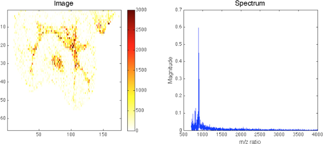
NMF component – main peak m/z 892.74.

The second spatial feature is not as crisp as the one found with ICA, but does have the same spectral peaks and a similar spectrum (Fig. 11).

Fig. 11.

NMF component – main peak m/z 1384.4827.

Like the ICA algorithm, NMF also isolates noise (Fig. 12). However, it produces two “noise” spectra for this dataset, rather than one as in ICA.

Fig. 12.

NMF component – noise spectrum.

NMF’s performance is very similar to that of ICA. It tends to have slightly cleaner spectra. Again, this is most likely a result of the segregation of spectral noise into separate components. The non-negative constraint of NMF ensures that results are purely additive, which makes the most sense from a physical perspective.

The main peaks of NMF components identify the three biological molecules: Sulfatide 20:0 (m/z 834.61), Sulfatide 24:0 (m/z 888.66), and Sulfatide 24:1 (m/z 890.66). The spectra containing these are very similar to those in ICA.

Discussion and Conclusions

Although all three methods isolated the same biological molecules, NMF and ICA produced components, with less noise in both the spectra and images. These algorithms require more computation time, but may be a better choice for IMS data exploration. The benefits of NMF versus ICA are not significant as far as spatial clarity and molecule separation are concerned.

The multivariate analysis techniques explained and explored here show excellent potential as methods for first examining an IMS dataset. They are able to rapidly identify and separate spatially significant and spectrally significant information. These initial interesting features can then guide a knowledgeable researcher in discovering relationships and biologically significant molecules in the dataset. Further research should be done with more datasets to better understand the effects of using different algorithms. The effectiveness of the different methods at isolating molecules and components in diseased versus healthy samples could also yield interesting results. If any one of the methods yielded a separate disease component, this could be helpful for other research applications.

References

- 1.Chaurand P, Schwartz SA, Reyzer ML, Caprioli RM. Imaging mass spectrometry: principles and potentials. Toxicol Pathol. 2005;33:92–101. doi: 10.1080/01926230590881862. [DOI] [PubMed] [Google Scholar]
- 2.Chen YF, Allegood J, Liu Y, Wang E, Cachon-Gonzalez B, Cox TM, Merrill AH, Sullards MC. Imaging MALDI mass spectrometry using an oscillating capillary nebulizer matrix coating system and its application to analysis of lipids in brain from a mouse model of Tay-Sachs/Sandhoff disease. Analytical Chemistry. 2008 Apr 15;80:2780–2788. doi: 10.1021/ac702350g. [DOI] [PubMed] [Google Scholar]
- 3.Muir ER, Ndiour IJ, Le Goasduff NA, Moffitt RA, Liu Y, Sullards MC, Merrill AH, Chen Y, Wang MD. Multivariate Analysis of Imaging Mass Spectrometry Data; Bioinformatics and Bioengineering, 2007. BIBE 2007. Proceedings of the 7th IEEE International Conference on; 2007. pp. 472–479. [Google Scholar]
- 4.Norris JL, Cornett DS, Mobley JA, Andersson M, Seeley EH, Chaurand P, Caprioli RM. Processing MALDI Mass Spectra to Improve Mass Spectral Direct Tissue Analysis. Int J Mass Spectrom. 2007 Feb 1;260:212–221. doi: 10.1016/j.ijms.2006.10.005. [DOI] [PMC free article] [PubMed] [Google Scholar]
- 5.Sjovall P, Lausmaa J, Johansson B. Mass spectrometric imaging of lipids in brain tissue. Analytical Chemistry. 2004 Aug 1;76:4271–4278. doi: 10.1021/ac049389p. [DOI] [PubMed] [Google Scholar]
- 6.Van de Plas R, De Moor B, Waelkens E. Imaging mass spectrometry based exploration of biochemical tissue composition using peak intensity weighted PCA. Life Science Systems and Applications Workshop, 2007. LISA 2007. IEEE/NIH. 2007:209–212. [Google Scholar]
- 7.McCombie G, Staab D, Stoeckli M, Knochenmuss R. Spatial and spectral correlations in MALDI mass spectrometry images by clustering and multivariate analysis. Analytical Chemistry. 2005 Oct 1;77:6118–6124. doi: 10.1021/ac051081q. [DOI] [PubMed] [Google Scholar]
- 8.Van de Plas R, Ojeda F, Dewil M, Van Den Bosch L, De Moor B, Waelkens E. Prospective exploration of biochemical tissue composition via imaging mass spectrometry guided by principal component analysis. Pac Symp Biocomput. 2007:458–469. [PubMed] [Google Scholar]
- 9.Hyvarinen A, Karhunen J, Oja E. Independent component analysis. New York: J. Wiley; 2001. [Google Scholar]
- 10.Scholz M, Gatzek S, Sterling A, Fiehn O, Selbig J. Metabolite fingerprinting: detecting biological features by independent component analysis. Bioinformatics. 2004 Oct 12;20:2447–2454. doi: 10.1093/bioinformatics/bth270. [DOI] [PubMed] [Google Scholar]
- 11.Wang GQ, Cai WS, Shao XG. A primary study on resolution of overlapping GC-MS signal using mean-field approach independent component analysis. Chemometrics and Intelligent Laboratory Systems. 2006 May 26;82:137–144. [Google Scholar]
- 12.Hyvarinen A, Oja E. A fast fixed-point algorithm for independent component analysis. Neural Computation. 1997 Oct 1;9:1483–1492. doi: 10.1142/S0129065700000028. [DOI] [PubMed] [Google Scholar]
- 13.Lee DD, Seung HS. Learning the parts of objects by non- negative matrix factorization. Nature. 1999 Oct 21;401:788–791. doi: 10.1038/44565. [DOI] [PubMed] [Google Scholar]
- 14.Lee DD, Seung HS. Algorithms for Non-negative Matrix Factorization. In: Leen TK, Dietterich TG, Tresp V, editors. Advances in Neural Information Processing Systems. Vol. 13. Cambridge, MA: MIT Press; 2001. pp. 556–562. [Google Scholar]
- 15.Fogel P, Young SS, Hawkins DM, Ledirac N. Inferential, robust non-negative matrix factorization analysis of microarray data. Bioinformatics. 2007 Jan 1;23:44–49. doi: 10.1093/bioinformatics/btl550. [DOI] [PubMed] [Google Scholar]
- 16.Gao Y, Church G. Improving molecular cancer class discovery through sparse non-negative matrix factorization. Bioinformatics. 2005 Nov 1;21:3970–3975. doi: 10.1093/bioinformatics/bti653. [DOI] [PubMed] [Google Scholar]
- 17.Gavert H, Hurri J, Sarela J, Hyvarinen A. The FastICA package for MATLAB. [Accessed: Aug 4, 2008]; [Online]. Available: http://www.cis.hut.fi/projects/ica/fastica/. [Google Scholar]
- 18.Hoyer P. nmfpack. [Accessed: Aug 4, 2008]; [Online]. Available: http://www.cs.helsinki.fi/u/phoyer/software.html. [Google Scholar]