Segmentation of organs‐at‐risks in head and neck CT images using convolutional neural networks

Abstract

Purpose

Accurate segmentation of organs‐at‐risks (OARs) is the key step for efficient planning of radiation therapy for head and neck (HaN) cancer treatment. In the work, we proposed the first deep learning‐based algorithm, for segmentation of OARs in HaN CT images, and compared its performance against state‐of‐the‐art automated segmentation algorithms, commercial software, and interobserver variability.

Methods

Convolutional neural networks (CNNs)—a concept from the field of deep learning—were used to study consistent intensity patterns of OARs from training CT images and to segment the OAR in a previously unseen test CT image. For CNN training, we extracted a representative number of positive intensity patches around voxels that belong to the OAR of interest in training CT images, and negative intensity patches around voxels that belong to the surrounding structures. These patches then passed through a sequence of CNN layers that captured local image features such as corners, end‐points, and edges, and combined them into more complex high‐order features that can efficiently describe the OAR. The trained network was applied to classify voxels in a region of interest in the test image where the corresponding OAR is expected to be located. We then smoothed the obtained classification results by using Markov random fields algorithm. We finally extracted the largest connected component of the smoothed voxels classified as the OAR by CNN, performed dilate–erode operations to remove cavities of the component, which resulted in segmentation of the OAR in the test image.

Results

The performance of CNNs was validated on segmentation of spinal cord, mandible, parotid glands, submandibular glands, larynx, pharynx, eye globes, optic nerves, and optic chiasm using 50 CT images. The obtained segmentation results varied from 37.4% Dice coefficient (DSC) for chiasm to 89.5% DSC for mandible. We also analyzed the performance of state‐of‐the‐art algorithms and commercial software reported in the literature, and observed that CNNs demonstrate similar or superior performance on segmentation of spinal cord, mandible, parotid glands, larynx, pharynx, eye globes, and optic nerves, but inferior performance on segmentation of submandibular glands and optic chiasm.

Conclusion

We concluded that convolution neural networks can accurately segment most of OARs using a representative database of 50 HaN CT images. At the same time, inclusion of additional information, for example, MR images, may be beneficial to some OARs with poorly visible boundaries.

1. Introduction

Head and neck (HaN) cancer including oral cavity, salivary glands, paranasal sinuses, and nasal cavity, nasopharynx, oropharynx, hypopharynx, and larynx cancers is among the most prevalent cancer types worldwide.¹ In the last decades, high‐precision radiation therapy such as intensity‐modulated radiation therapy (IMRT), volumetric‐modulated radiation therapy (VMAT), and proton therapy have been widely used for HaN cancer treatment due to their ability for highly conformal dose delivery. To minimize post‐treatment complications, organs‐at‐risks (OARs), such as brainstem, spinal cord, mandible, larynx, pharynx, parotid, and submandibular glands, and, in the case of nasopharyngeal cancer, eyes, optic nerves, and chiasm, must be accurately delineated. The complexity of OARs morphology and imperfection of imaging devices make manual delineation prone to errors and time consuming.² There is therefore a great demand for more accurate OAR delineation and for considerable reduction in the amount of manual labor in HaN treatment planning.³

Computed tomography (CT)‐based treatment planning remains to be the mainstay in current clinical practice for its high acquisition speed, high spatial accuracy and resolution, and the ability to provide relative electron density information. However, CT images have low contrast of soft tissues and are usually corrupted by metallic artifacts which limit applicability of intensity‐based segmentation algorithms. As the general appearance of OARs and surrounding tissues remains similar among CT images of different patients, there is a certain confidence that previously analyzed training images can be used to segment a new test image. The most straightforward approach is to align, that is, register, training images, so‐called atlases, to the test image and correspondingly propagate the training OAR annotations. Such atlasing has been receiving considerable attention in the literature on HaN segmentation.³ Nonrigid registration of three‐dimensional (3D) images is a relatively slow procedure, therefore early HaN segmentation methods registered a single atlas with annotation to the test image.^{4, 5, 6} This atlas was usually defined using an arbitrary training image, which negatively affected registration performance if the selected image was not representative.^{4, 6, 7} Such bias can be reduced when the atlas is defined using an artificial image with standard anatomy^{8, 9} or the average image constructed by merging several training images.^{5, 10, 11} It is also possible to choose a new atlas image for every segmentation according to its similarity to the test image.¹² A single atlas, however, cannot guarantee accurate segmentation results in the presence of pathologies and tumors when the morphology of OARs is not similar enough between the atlas and test image. Multiatlas segmentation is less sensitive to interpatient anatomy variability and produces more accurate segmentation results if a high number of atlas images are used.^{13, 14, 15} The registrations for all atlases are usually combined with simultaneous truth and performance level estimation (STAPLE),¹⁶ similarity and truth estimation (STEPS)¹⁶ and joint‐weighted voting¹⁷ techniques. When validated on HaN muscles, lymph nodes, spinal cord, and brainstem, multiatlas segmentation was shown to be slower but more accurate than single atlas segmenation.¹² Apart from atlas selection, the results strongly depend on the parameters of the applied registration algorithm. In the literature, registration of two HaN images was based on simple intensity‐,¹⁸ mutual information‐,^{4, 15, 19, 20, 21} and Gaussian local correlation coefficient‐based⁴ similarly measures, and optical flow,⁸ consistent volumes,²² scale‐invariant features,²³ locally affine block matching,^{5, 10, 16} demons,²⁴ fluid dynamics²⁵ radial basis function²⁶, and B‐splines^{11, 13, 15, 20} for controlling registration transformations. It was also concluded that HaN registration convergence improves considerably when anchor landmarks located at anatomically relevant regions such as vertebrae and mandible corners are used.^{20, 27, 28} Landmark‐assisted atlasing demonstrated better performance in comparison to standard atlasing on segmentation of lymph nodes,²⁰ brainstem,²⁷ and individual tongue muscles.²⁸

Alternative HaN segmentation approaches applied fast marching,²⁹ mass springs for lymph nodes modeling³⁰ parametrical shapes for eye globes and optical nerve modeling,³¹ active contours,³² deformable meshes,^{24, 33} principal component‐based shapes,^{11, 19} graph cut,^{13, 17} and superpixels.¹⁵ In general, shape‐based approaches demonstrated exceptional performance on segmentation of heart³⁴ and spine,^{35, 36, 37} and annotation of X‐ray head images.^{38, 39} Researchers also studied the performance of machine learning algorithms such as k‐nearest neighbors and support vector machines trained on intensity, gradient, texture contrast, texture homogeneity, texture energy, cluster tendency, Gabor and Sobel features.^{21, 24} The above mentioned algorithms covered the complete set of OARs in the HaN region including brainstem,^{4, 7, 8, 9, 10, 11, 12, 14, 16, 17, 18, 24, 25, 26, 27, 40, 41} cerebellum,^{9, 13, 14, 17, 25, 41} spinal cord,^{4, 13, 16, 18, 40, 41} mandible,^{4, 10, 18, 24, 42, 43, 44, 45} parotid glan‐ds,^{4, 7, 10, 11, 15, 16, 18, 21, 24, 33, 40, 44, 46} submandibular glands,^{4, 24, 46} pituitary gland,⁹ thyroid,^{13, 41, 47} eye globes,^{9, 13, 14, 17, 31, 40, 41} eye lenses,^{13, 14, 16, 17, 41} optic nerves,^{5, 9, 14, 26, 31, 41} optic chiasm,^{5, 9, 16, 26, 31} larynx,^{40, 46} pharyngeal constrictor muscle,^{46, 48} pterygoid muscles,⁴ tongue muscles,²⁸ and lymph nodes.^{4, 6, 12, 18, 19, 20, 24, 25, 29, 30, 32, 49} Despite the considerable attention, the demonstrated results are still not satisfactory for the clinical usage and automated methods cannot accurately segment OARs in the presence of tumors and severe pathologies.

In the work, we propose the first deep learning‐based algorithm for HaN CT image segmentation. Deep learning techniques such as convolutional neural networks (CNNs) have demonstrated impressive performance in computer vision and medical image analysis applications.⁵⁰ Being supervised, CNNs first study the appearance of objects of interest in a training set of segmented images. When a previously unseen test image arrives, CNNs mark the voxels that have an appearance similar to the corresponding OARs. The performance of CNNs was validated on segmentation of spinal cord, mandible, parotid glands, submandibular glands, larynx, pharynx, eye globes, optic nerves, and optic chiasm. The paper is organized as follows.

Section 2 presents the theoretical concept of CNNs and the way we used CNNs for image segmentation. In Section 3, we described a validation database of HaN CT images and the results of CNN‐based segmentation. We compared the results with state‐of‐the‐art in Section 4, and concluded in Section 5.

2. Methods

2.A. Convolutional neural networks

Convolutional neural network is a special kind of multilevel perceptron architecture, where an input image passes through a sequence of classification tests that can extract and recognize its consistent intensity patterns and finally make a prediction about the image according to these patterns. In contrast to alternative machine learning‐based algorithms, CNNs take spatial information into account so that neighboring pixels are analyzed together. This behavior combined with abilities for generalization makes CNNs superior to other approaches on a number of computer vision applications, such as handwritten text recognition, face detection and object classification.⁵¹ A CNN is organized as a set of different layers, where output of a current layer is used as an input for the next layer. A convolution layer—the main component of CNNs—serves to generate a predefined number of rectangular features computed from the output of the previous layer or the original image, if this convolution layer is positioned at the beginning of a CNN. As a result, convolution layers extract elementary features of the input such as edges and corners, which after passing through next layers are combined into more complex high‐order features. A convolutional layer is usually followed by a rectified linear units (ReLU), hyperbolic tangent, or sigmoid layer that introduces nonlinearity to the convolution layer response and reduces overfitting and vanishing or exploding gradient effects. A pooling layer then partitions the input into nonoverlapping rectangles and returns the maximum or average value of each rectangle. This makes CNNs more robust against local transformations of the input as pooling layers are invariant to small shift, rotation and scaling. Moreover, pooling considerably reduces the input size and consequently the number of network parameters, and therefore prevents CNN overfitting. Standard networks composed of convolution‐ReLU‐pooling layer sets are sometimes sensitive to initialization and require fine parameters tuning in order to avoid gradient explosions. The recent study has demonstrated that batch‐based normalization (bNorm) of each convolution layer makes networks less sensitive to input parameter initialization and increases network convergence more than 14 times.⁵² Finally, the robustness of the network can be improved by random removal of some neurons, which is performed using dropout layers.⁵³ After a sequence of convolution‐bNorm‐ReLU‐dropout‐pooling layer sets, the input image shrinks into a small set of high‐order features and finally passes through fully connected layers that generate the network output (Fig. 1).

Figure 1.

A schematic illustration of the convolutional neural network architecture. Three orthogonal cross‐sections around target voxel define the input of the network that consists of three stacks of convolution, ReLU, max‐pooling layer, and dropout layers, fully connected and softmax layers.

In order to use CNNs for image annotation, let us have a training set T of 3D images with an object (objects) of interest annotated. An image patch of each voxel that belongs to the object of interest contains some intensity patterns that make it distinguishable from the patches of other voxels in the image. The goal of a CNN is to correctly capture these patterns, and use them to identify object voxels in unseen images. As it was shown in the recent studies, CNNs trained on a set of tri‐planar patches, that is, square intensity neighborhoods extracted at three orthogonal cross‐sections and centered at the target voxel, exhibit similar segmentation performance but dramatic acceleration in comparison to CNNs trained on 3D patches.⁵⁴ We therefore designed a tri‐planar patch‐based network with three sets of convolution‐bNorm‐ReLU‐dropout‐pooling layers, a fully connected layer and a softmax layer that converts network output into classification prediction values (Fig. 1).

2.B. Detection of organs‐at‐risks

In the training set T of HaN CT images, experienced clinicians defined objects of interest as OARs including spinal cord, mandible, parotid glands, submandibular glands, eye globes, optic nerves, optic chiasm, larynx, and pharynx. The goal is to detect and segment these OARs in a previously unseen target image. Although initial OAR detection is not mandatory, it considerably reduces segmentation computational costs as only voxels that may geometrically belong to OARs are analyzed. For this aim, we automatically detect the patient's head, which is used as a reference point for approximation of OAR positions. Following the geometry of the human head, we observe that the image gradients computed at skull boundaries are, in general, oriented toward the brain center, which allow us to apply the existing algorithm developed for detection of spherical structures, such as femoral heads.⁵⁵ For every voxel $\mathbf{x}$ with gradient magnitude $|\mathrm{\nabla }{I}_{\mathbf{x}}|$ above a certain threshold, indicating that voxel x may belong to skull surface, we compute both positive$\mathrm{\nabla }{I}_{\mathbf{x}}$ and negative $-\mathrm{\nabla }{I}_{\mathbf{x}}$ gradient vectors. A high number of these gradient vectors intersect around the center of the skull, as a high number of gradients $\mathrm{\nabla }{I}_{\mathbf{x}}$ and $-\mathrm{\nabla }{I}_{\mathbf{x}}$ are oriented toward the head center (Fig. 2). We therefore search for the reference voxel where the number of intersected gradients is the highest, and define it as the head center. The regions of interest for each OAR are approximated according to this center point.

Figure 2.

The strongest gradients of the target CT image (first raw) intersect around the center of the patient's skull (second raw).

2.C. CNN‐based segmentation of head and neck CT images

To segment each object on a previously unseen test image, the corresponding CNN must be trained to recognize the intensity appearance of voxels that belong to the object and distinguish it from the intensity appearance of surrounding background voxels. During the network training phase for a selected object of interest $\mathcal{S}$, we extracted a set ${\mathcal{P}}_I^{+}$ of $\mathit{\kappa }$ voxels randomly sampled with repetitions from the set of voxels that belong to the binary mask that represents object $\mathcal{S}$ in image $I\in T$. A set ${\mathcal{P}}_I^{-}$ of the same cardinality of $\mathit{\kappa }$ voxels is randomly sampled with repetitions from voxels that do not belong to object $\mathcal{S}$ but are located not closer than $r$ mm from the nearest object voxel in image $I\in T$. We do not consider voxels that are located further than $R$ mm from object $\mathcal{S}$ because its position is restricted according to the patient anatomy and imaging protocol, and very distant voxels will therefore not be analyzed during segmentation and cannot enrich the corresponding CNN. For each voxel from ${\mathcal{P}}_I^{+}({\mathcal{P}}_I^{-})$, we extract tree orthogonal patches from image $I$ that define a positive (negative) training sample. A complete set of $\mathit{\kappa }·|T|$ positive and $\mathit{\kappa }·|T|$ negative training samples, generated for all images from $T$, is used by CNN for modeling the intensity appearance pattern that separates object $\mathcal{S}$ from background⁵⁶ (Fig. 3). The trained network is next applied to classify voxels in the region of interest of the test image where the corresponding OARs are expected to be located. The classification result of the network computed for a voxel $\mathbf{x}$ passes through the softmax layer to obtain the probability ${\mathcal{P}}_{\mathbf{x}}^{\mathcal{S}}$ that voxel x belongs to object $\mathcal{S}$.

Figure 3.

A schematic set of parameters and commands used to define convolutional neural network for segmentation of organ‐at‐risks in head‐and‐neck CT images. The parameters in bold correspond to the size of convolution and pooling layers.

2.D. Markov random fields and segmentation postprocessing

Segmentation with CNNs usually produces smooth probabilities ${\mathcal{P}}_{\mathbf{x}}^{\mathcal{S}}$ because voxels located close to each other have a similar intensity appearance. However, CNNs do not explicitly incorporate voxel connectivity information and the morphology of OARs. As the morphology of OARs strongly depends on the location of the tumor and is often poorly predictable, we rely on connectivity information and apply Markov random fields (MRF) to improve CNN results. According to the MRF formulation, the target 3D image can be described as a graph $\mathcal{G}=\{\mathcal{V},\mathit{\epsilon }\}$, where vertices $\mathcal{V}$ correspond to image voxels, and edges $\mathit{\epsilon }$ connect vertices that correspond to neighboring voxels. For each object $\mathcal{S}$, each vertex can be assigned label 1 if it belongs to $\mathcal{S}$, and assigned 0 otherwise. The label of a voxel depends on its similarity to object $\mathcal{S}$, that is, probability ${\mathcal{P}}_{\mathbf{x}}^{\mathcal{S}}$, and similarity to object $\mathcal{S}$ of its neighbors:

$$L^{\mathcal{S}}=\text{arg}\underset{l_{\mathbf{x}}}{min}\left(\sum _{\mathbf{x}\in \mathcal{V}}\mathit{\varphi }({\mathcal{P}}_{\mathbf{x}}^{\mathcal{S}},l_{\mathbf{x}})+\sum _{(\mathbf{x},\mathbf{y})\in \mathit{\epsilon }}{\mathit{\psi }}_{\mathbf{x},\mathbf{y}}\mathrm{\Delta }(l_{\mathbf{x}},l_{\mathbf{y}})\right),$$

where function $\mathit{\varphi }\left({\mathcal{P}}_{\mathbf{x}}^{\mathcal{S}},l_{\mathbf{x}}\right)=\left(l_{\mathbf{x}}==1\right)?1-{\mathcal{P}}_{\mathbf{x}}^{\mathcal{S}}:{\mathcal{P}}_{\mathbf{x}}^{\mathcal{S}}$ defines the cost of assigning label 1 to voxel $\mathbf{x}$ as $1-{\mathcal{P}}_{\mathbf{x}}^{\mathcal{S}}$, and the cost of assigning label 0 to voxel $\mathbf{x}$ as ${\mathcal{P}}_{\mathbf{x}}^{\mathcal{S}}$. Function ${\mathit{\psi }}_{\mathbf{x},\mathbf{y}}=\exp (-\frac{{({\mathcal{P}}_{\mathbf{x}}^{\mathcal{S}}-{\mathcal{P}}_{\mathbf{y}}^{\mathcal{S}})}^2}{2{\mathit{\sigma }}^2})$ measures similarity between probabilities ${\mathcal{P}}_{\mathbf{x}}^{\mathcal{S}}$ and ${\mathcal{P}}_{\mathbf{y}}^{\mathcal{S}}$ of voxels x and y, respectively, and $\mathrm{\Delta }(l_{\mathbf{x}},l_{\mathbf{y}})$ is an indicator function that equals 0 if labels $l_{\mathbf{x}}==l_{\mathbf{y}}$, and equals 1 otherwise. The first term of Equation 1 tries to assign voxel labels according to the probabilities ${\mathcal{P}}_{\mathbf{x}}^{\mathcal{S}}$ computed by the CNN, whereas the second term tries to make labels of all neighboring voxels, that is, labels of all voxels in the image, the same. Searching for the equilibrium between these two terms usually makes the resulting label mask smooth and suppresses both small groups of voxels with high probabilities ${\mathcal{P}}_{\mathbf{x}}^{\mathcal{S}}$ surrounded by voxels with low probabilities ${\mathcal{P}}_{\mathbf{x}}^{\mathcal{S}}$, and vice versa. For solving this MRF, we used a publicly available software FastPD, which can find the optimal MRF‐based labeling almost in real time.⁵⁷

Despite its effectiveness, MRF approach cannot suppress large groups of isolated voxels, and fill large cavities in resulting label maps $L^{\mathcal{S}}$. However, we know in advance that OARs represent solid connected structures with smooth boundaries, and should not be separated into several components and do not have internal cavities. We therefore extract the largest connected component of voxels $L^{\mathcal{S}}$ so that noise voxel groups with probability $l_{\mathbf{x}}>0.5$ are removed. A sequence of dilation operations is then used to fill all the cavities in the obtained largest component. The same number of erosion operations compensate for the overexpansion of the dilated component, which finally defines segmentation of object $\mathcal{S}$ in the test image. After performing CNN‐based voxel classification, MRF‐based smoothing, small component removal, and dilate–erode operations for all objects of interest, segmentation of the test image is complete.

3. Experiments and results

3.A. Image database

We collected 3D CT images of 50 patients scheduled for head and neck radiotherapy. All images were axially reconstructed and had an in‐plane resolution between 0.781 and 1.310 mm with the scan matrix of 512 × 512, whereas the slice thickness varied between 1.5 and 2.5 mm. Experienced radiologists annotated mandible in 48 images; optic nerves and right eye globe in 47 images; left parotid, left eye globe, and chiasm in 46 images; spinal cord, right parotid, and larynx in 45 images; pharynx in 39 images; and both submandibular glands in 31 images, which rounds to 563 objects to segment. Inclusion of certain OARs into the treatment planning procedure depended on the position of the tumor and image field of view.

3.B. Validation

We performed a five‐fold cross‐validation, where, for example, for segmenting the image with number 15, images with numbers 1–10 and 21–50 were used for CNN training. During the training phase, all voxels thatbelong to the reference segmentations of OARs were extracted. For each OAR mask and its surrounding structures, we randomly subsampled $\mathit{\kappa }=$ 25000 positive and $\mathit{\kappa }=$ 25000 negative patches of 27 × 27 × 3 size, that is, axial, sagittal, and coronal patches of 27 × 27 mm, that formed the training set of samples for the corresponding image. The negative samples were located not closer than $r=$ 2 mm and not further than $R=$ 40 mm from the surface of the corresponding OARs. According to the positive and negative samples from all training images, the networks were optimized using the stochastic gradient descent scheme, initialized with a learning rate of 0.0005 and momentum of 0.9. An additional gradient clipping procedure is used to prevent gradient explosions, which sometimes occur during CNN training. The training samples were separated into batches with 250 samples each, and all batches were analyzed in 25 epochs, that is, training procedure runs 25 times through all training samples. The binary masks obtained after performing CNN‐based voxel classification, small component removal, and dilate–erode operations were compared to reference segmentation masks by computing the true positive (TP) rate that is the number voxels classified as the target OAR in both reference and automated segmentation, and the false positive (FP) rate that is the number of voxels misclassified as the target OAR by automated segmentation, and false negative (FN) rate that is the number of OAR voxels misclassified as background by automated segmentation. In the case of spinal cord segmentation, we did not consider automatic segmentation on the slices depicting thoracic spine where the spinal cord is not segmented by the clinicians. The intuition is that the reference segmentation of spinal cord does not continue through the whole vertebral column, and stops at the slice where the cord is not affected anymore during the treatment. At the same time, automatic segmentation continues segmenting the spinal cord beyond this slice, which does not harm the treatment planning and shall not be straightforwardly considered as an error. The segmentation error was numerically measured using Dice coefficient (DSC) $=2TP/(2TP+FN+FP)$. The mean DSC varied from 37.4% for chiasm segmentation to 89.5% for mandible segmentation (Table 1 and Figs. 4 and 5).

Table 1.

Results of convolutional neural network‐based segmentation of organs‐at‐risks in head and neck CT images, given in terms of mean (± standard deviation) Dice coefficient (DSC)

Organ	DSC (%)
Spinal cord	87.0 ± 3.2
Mandible	89.5 ± 3.6
Parotid left	76.6 ± 6.1
Parotid right	77.9 ± 5.4
Submandibular left	69.7 ± 13.3
Submandibular right	73.0 ± 9.2
Larynx	85.6 ± 4.2
Pharynx	69.3 ± 6.3
Eye globe left	88.4 ± 2.7
Eye globe right	87.7 ± 3.7
Optic nerve left	63.9 ± 6.9
Optic nerve right	64.5 ± 7.5
Chiasm	37.4 ± 13.4

Figure 4.

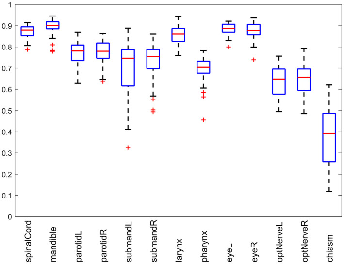
Box plot results of convolutional neural network‐based segmentation of organs‐at‐risks in head and neck CT images reported in terms of Dice coefficient.

Figure 5.

Segmentation results for three (a–c) selected head and neck CT image, shown in four axial cross‐sections. The reference segmentations are depicted in green and convolution neural network‐based segmentations are depicted in red.

3.C. Computation performance

The proposed algorithm uses two publicly available toolboxes: Computational Network Toolkit (CNTK)⁵⁶ and FastPD,⁵⁷ and a set of functions for pre‐ and postprocessing, which we implemented in C++ and executed on a personal computer with Intel Core i7 processor at 4.0 GHz and 32 GB of memory. A graphical processing unit (GPU) was used by CNTK for deep learning‐based segmentation. The training of the networks took 30 min per OARs, which rounds to 6.5 h for training 13 networks for all OARs. The analysis of one image took around 4 min, where only 1.5 min were used for deep learning classification of testing patches 2.5 min were used for reading‐writing of images and samples, OARs detection, image transformation, and postprocessing operations, whereas MRF refinement required less than a second.

4. Discussion

We presented the first attempt to use CNNs for segmentation of OARs from HaN CT images. As a number of automated and semiautomated methods have been proposed to address this problem, we compared our results with the current state‐of‐the‐art and devised conclusions about the potential of using CNN for HaN radiotherapy planning. Segmentation of an OAR strongly depends on its size, shape, clarity of boundaries, presence of pathologies, and overall visibility in the CT image modality. The comprehensive comparison should be based not only on the results of existing automated segmentation methods but also on the performance of commercially available software and interobserver variability. We summarize research published on the topic of HaN OARs segmentations, compare the reported results with the proposed framework performance and identify baselines and milestones for individual OARs. We also present the interobserver variability for some OARs reported in the literature, which is important for the estimation of the complexity of the segmentation problem. However, it is important to mention that this is not the direct comparison obtained on the same database, but the results of alternative automated methods, commercial software, and human performance reported on different databases.

4.A. Spinal cord segmentation

Radiation therapy can cause toxicity to the nervous system, if spinal cord is affected during the treatment. This can lead to self‐limited transient or progressive myelopathy, or, in rare cases, to lower motor neuron syndrome. As the spinal cord is poorly visible in CT images, clinicians usually segment the region encompassed by vertebral foramens that ensures some safe margins for spinal cord. Although the surface of cervical vertebrae is a guide for segmentation, identification of the exact boundaries of spinal cord in the test CT image is a challenging task. Existing automated segmentation methods reported Dice coefficient of 62%,¹⁶ 75%,¹⁶ 76%,⁴¹ 78%,⁴ 83%,¹⁸ and 85%.¹³ La Macchia et al.⁴⁵ measured the performance of commercial software on spinal cord segmentation and obtained Dice coefficient of 70% 81%, and 78% for VelocityAI 2.6.2, MIM 5.1.1, and ABAS 2.0 systems, respectively. To objectively estimate the complexity of the problem, it is important to mention that interobserver variability was reported to be of 77%,⁴⁸ 79%,^{40, 41} 80%⁵⁸ DSC 60%⁵⁹ in terms of conformity level, and 78%,⁶⁰ and 89%⁶¹ in terms of maximal volume difference. We can therefore conclude that the proposed CNN‐based spinal cord segmentation result of 87.0 ± 3.2% DSC compares favorably against the existing segmentation algorithms, commercial software, and interobserver variability (Fig. 5). This achievement can be explained by the fact that spinal cord has a very consistent intensity pattern that can be accurately modeled by machine learning approaches such as CNNs. On the other hand, atlas‐based algorithms are often too restricted by the registration regularization, so that the resulting transformation field is smooth and not distorted but, at the same time, atlasing cannot perfectly capture variable curvature of the spine, cervical vertebra sizes, etc.

4.B. Mandible segmentation

Irradiation of dental area can cause dental decay, postextraction osteoradionecrosis, and implant failure, therefore, the mandible has to be spared during the HaN radiotherapy procedure.⁴³ Mandible identification is facilitated by its relatively large size and rigid shape, whereas the fact that mandible has a better contrast in CT images in comparison to the surrounding soft structures simplifies its segmentation. The main challenge is the presence of severe image artifacts around the teeth due to metallic dental restorations. These artifacts hamper correct identification of mandible borders and often corrupt the appearance of the surrounding structures such as tongue, parotid, and submandibular glands. These artifacts were, in general, excluded from mandible segmentation, as CNNs were able to correctly model the composition of dark and bright voxel groups that usually characterize dental artifacts in CT images. Moreover, the teeth region where dental artifacts are manifested was not included into manual segmentation, which additionally supported automated segmentation. Automated mandible segmentation has received considerable attention in the research community, and the obtained results measured in terms of Dice coefficient were of 78%,⁶² 80%,⁴ 82%,^{10, 44} 86%,¹⁸ 90%,¹⁰ and 93%^{24, 42}, whereas existing commercial VelocityAI 2.6.2, MIM 5.1.1, and ABAS 2.0 software systems demonstrated Dice coefficient of 84% 86%, and 89%, respectively. The proposed CNN‐based algorithm segmented mandible with 89.5 ± 3.6% DSC, which is comparable with the best performing segmentation algorithms (Fig. 5, 2^nd and 3^rd rows). Moreover, the demonstrated results are similar to the semiautomatic segmentations with 89%⁴⁵ DSC, and interobserver variability of 87%⁵⁸ and 89%⁴⁰ DSC.

4.C. Parotid and submandibular gland segmentation

Xerostomia—changes in volume, consistency, and pH of saliva—is one of the main complications after HaN radiation therapy.⁶³ As around 60% and 30% of saliva is produced by parotid or submandibular glands, xerostomia is usually manifested when these glands are irradiated during treatment.⁶³ Segmentation of parotid or submandibular glands in CT images is challenging due to their irregular shapes and poorly visible boundaries that are additionally corrupted by dental artifacts. According to literature overview, automated segmentation results of 57%,¹⁶ 65%,¹⁶ 68%,¹⁰ 72%,⁷ 77%,³³ 79%,^{40, 44} 80%,^{4, 18, 46} 83%,^{4, 15, 24} 84%,¹¹ 85%¹⁰ DSC for parotid glands, and 70%,⁴ 80%,⁴⁶ and 83%²⁴ DSC for submandibular glands were reported. At the same time, VelocityAI 2.6.2, MIM 5.1.1, and ABAS 2.0 software systems demonstrated parotid gland segmentation performance of 73% 79%, and 79% DSC, respectively.⁴⁵ The agreement among radiologists is slightly better than between automated and manual segmentation and is reported to be of 76%,⁵⁸ 79%,⁴⁰ 85%,³³ and 90%⁴⁶ DSC, and 77%⁶¹ volume difference for parotid glands, and 91%⁴⁶ DSC and 77%⁶⁰ volume difference of submandibular glands. The results of the proposed algorithm are of 77.3 ± 5.8% DSC for both parotid glands, which is comparable with the average results of the existing segmentation methods and above average in comparison to the performance of the commercial software (Fig. 5). Manual segmentation results indicate that parotid glands may be challenging to annotate even for a human. Moreover, parotid glands are often affected by pathologies, which considerably reduces the reliability of segmentation. The results of the proposed algorithm are of 71.4 ± 11.6% DSC for submandibular glands, which is lower than the average performance of existing algorithms, and commercial software (Fig. 4, 2^nd and 3^rd rows). There are two reasons why CNNs are not as effective as atlas‐based segmentation for submandibular glands. First, the glands do not have very distinguishable intensity features that would make them different from the surrounding structures in contrast to spinal cord and mandible. Second, atlasing deformation is relatively restricted, and therefore, even if a gland cannot be perfectly recognized, atlasing can still roughly identify the gland positioning. At the same time, CNN relies purely on image intensities around glands, and therefore may sometimes get confused. The positive consequence of this property is that segmentation of abnormal submandibular gland is going to be more challenging for atlasing, as it cannot efficiently incorporate the tumor position. We also observe that submandibular gland segmentation accuracy strongly depends on the particular image database, and even human performance can vary dramatically.

4.D. Larynx and pharynx

Dysphagia or swallowing dysfunction is considered to be the second most commonly occurring complication of the HaN radiation therapy.⁶³ The manifestation of dysphagia has been shown to be consistently caused by irradiation of supraglottic larynx and pharyngeal constrictor muscles.⁶³ Although segmentation of larynx and pharynx is often required for treatment planning, automated segmentation of them has not been receiving as much attention as segmentation of spinal cord, mandible, and glands, due to highly variable intensity of larynx and poorly defined boundaries and complex shape of pharynx in CT images. To the best of our knowledge, the existing studies on the topic reported automated segmentation results of 58%⁴⁶ and 73%⁴⁸ DSC for larynx and 50%⁴⁶ and 64%⁴⁸ DSC for pharyngeal constrictor muscles. Commercial VelocityAI 2.6.2, MIM 5.1.1, and ABAS 2.0 software systems demonstrated better performance of 81% 83%, and 84% DSC, respectively, on larynx segmentation, and 63% 66%, and 65% DSC, respectively, on pharynx segmentation.⁴⁵ Clinicians demonstrated an agreement of 60%⁴⁸ and 83%⁴⁰ DSC for larynx segmentation. We obtained segmentation results of 85.6 ± 4.2% DSC for larynx and 69.3 ± 6.3% DSC for pharynx that is superior or comparable to the best performing automated segmentation and interobserver variability (Fig. 5, 2^nd–4^th rows). Designed CNNs were therefore able to correctly capture the appearance of laryngeal cartilages and pharyngeal area that is surrounded by cervical spine and airways.

4.E. Eyes, optical nerves and chiasm

In the case of nasopharyngeal cancer, tumors can be located in the close proximity to human vision system, irradiation of which can cause serious complications such as radiation‐induced optic neuropathy.⁶⁴ Modern HaN radiotherapy protocols therefore require preoperative annotation of eye globes, optical nerves, and chiasm. Eyes have well‐defined spherical shape and, despite poor visibility of the globe surface in CT images, can be accurately segmented with 80%^{13, 41} and 81%⁹ DSC using atlas‐ and model‐based algorithms. The optic nerves, which are thin elongated structures that start at the eyes and meet below the hypothalamus, can be automatically segmented with 38%,⁹ 58%,⁴¹ 42%,¹³ and 61%¹³ DSC. The optic nerve intersection, that is, optic chiasm, has a very small size and poorly visible boundaries and can be segmented automatically with relatively low accuracy of 39%²⁶ and 41%⁹ DSC. Similar to the results of automated segmentation, interobserver agreement is higher for eye globes, namely 86%^{26, 41} and 89%⁴⁰ DSC, lower for optic nerves, namely 51%,²⁶ 57%,⁴⁸ and 60%⁴¹ DSC, and the lowest for optic chiasm, namely 38%⁴⁸ and 41%²⁶ DSC. The proposed CNN‐based algorithm with 88.0 ± 3.2% DSC outperforms the existing state‐of‐the‐art algorithms for eye globe segmentation, with 64.2 ± 7.2% DSC similar to the best performing algorithm¹³ for optic nerve segmentation, but with 37.4 ± 13.4% DSC, which is worse than the existing algorithms for chiasm segmentation (Fig. 5, 1^st row).

4.F. Methodological comparison

As a supervised technique, CNNs considerably relie on the quality and representativeness of the training data. The richer the training dataset is, the more accurate and reliable segmentation is, which, however, does not affect computational time of CNN‐based segmentation. In contrast, the computational complexity of multi‐image atlasing linearly increases with the number of training images so that the target image may require hours to be segmented. The training phase of CNNs is relatively lengthy but happens only once and therefore does not affect segmentations of individual target images. For both CNNs and atlasing, segmentation accuracy is often lower for OARs located close to tumors. Indeed, the tumor presence changes the appearance and morphology of the OARs and the consistent appearance patterns learned by CNNs become less representative. This issue is more pronounced in the case of atlasing, as registering an image with no tumor at a specific location to an image with tumor at this location is extremely challenging. On the other hand, image artifacts and local intensity inhomogeneity are more destructive for CNNs than for atlasing. Similarly, as in the case of tumor positioning, patterns learned by CNNs become less representative, whereas artifacts and intensity inhomogeneity does not affect the morphology of OARs, and therefore altasing is still able to perform registration.

Finally, we want to estimate the contribution of the MRF‐based smoothing on framework performance. Having CNN‐based classifications, MRF smoothen the surface of the resulting binary masks and remove isolated misclassified voxels or groups of voxels. The performance improvement was therefore lower for objects with clearly visible boundaries, for example, mandible segmentation was improved by 0.24 Dice, and well‐defined shape, for example, left and right eye globe segmentations were improved by 0.45 and 0.03 Dice, respectively. At the same time, CNNs produced irregular segmentation for poorly visible left and right submandibular glands, therefore, the contribution of MRF was considerable and resulted in segmentation improvement by 3.73 and 3.93 Dice respectively. On average, MRF increased the Dice coefficient by 0.91 for all OARs and visually improved segmentation boundaries.

5. Conclusion

In this paper, we presented the first attempt of using deep learning concept of convolutional neural networks for segmentation of OARs in the head and neck CT images. We observed that CNNs demonstrated performance superior or comparable to the state‐of‐the‐art on segmentation of spinal cord, mandible, larynx, pharynx, eye globes, and optic nerves, and inferior performance on segmentation of parotid glands, submandibular glands, and optic chiasm. These results confirm that CNNs well‐generalize the intensity appearance of objects with recognizable boundaries, for example, spinal cord, mandible, pharynx, and eye globes. For the objects with poorly recognizable boundaries, for example, submandibular glands and optic chiasm, additional information may be required for CNN‐based segmentation. Following the clinical procedure, magnetic resonance images, which have better image contrast of soft tissues than CT image, can be included as an information source. However, this inclusion requires accurate multimodal registration of magnetic resonance to CT images, which is a very nontrivial task when images have different fields of view and resolution. Combining CT and magnetic resonance images may have potential but is not straightforward. In general, we confirm a high potential of deep learning for HaN image segmentation.

References

- 1. Torre LA, Bray F, Siegel RL, Ferlay J, Lortet‐Tieulent J, Jemal A. Global cancer statistics 2012. CA Cancer J Clin. 2015;65:87–108. [DOI] [PubMed] [Google Scholar]
- 2. Harari PM, Song S, Tomé WA. Emphasizing conformal avoidance versus target definition for IMRT planning in head‐and‐neck cancer. Int J Radiat Oncol Biol Phys. 2010;77:950–958. [DOI] [PMC free article] [PubMed] [Google Scholar]
- 3. Sharp G, Fritscher KD, Pekar V, et al. Vision 20/20: perspectives on automated image segmentation for radiotherapy. Med Phys. 2014;41:50902. [DOI] [PMC free article] [PubMed] [Google Scholar]
- 4. Han X, Hoogeman MS, Levendag PC, et al. Atlas‐based auto‐segmentation of head and neck CT images. Med Image Comput Comput‐Assist Interv MICCAI Int Conf Med Image Comput Comput‐Assist Interv. 2008;11:434–441. [DOI] [PubMed] [Google Scholar]
- 5. Commowick O, Grégoire V, Malandain G. Atlas‐based delineation of lymph node levels in head and neck computed tomography images. Radiother Oncol J Eur Soc Ther Radiol Oncol. 2008;87:281–289. [DOI] [PubMed] [Google Scholar]
- 6. Voet PWJ, Dirkx MLP, Teguh DN, Hoogeman MS, Levendag PC, Heijmen BJM. Does atlas‐based autosegmentation of neck levels require subsequent manual contour editing to avoid risk of severe target underdosage? a dosimetric analysis. Radiother Oncol J Eur Soc Ther Radiol Oncol. 2011;98:373–377. [DOI] [PubMed] [Google Scholar]
- 7. Daisne J‐F, Blumhofer A. Atlas‐based automatic segmentation of head and neck organs at risk and nodal target volumes: a clinical validation. Radiat Oncol Lond Engl. 2013;8:154. [DOI] [PMC free article] [PubMed] [Google Scholar]
- 8. Bondiau PY, Malandain G, Chanalet S, et al. Atlas‐based automatic segmentation of MR images: validation study on the brainstem in radiotherapy context. Int J Radiat Oncol Biol Phys. 2005;61:289–298. [DOI] [PubMed] [Google Scholar]
- 9. Isambert A, Dhermain F, Bidault F, et al. Evaluation of an atlas‐based automatic segmentation software for the delineation of brain organs at risk in a radiation therapy clinical context. Radiother Oncol J Eur Soc Ther Radiol Oncol. 2008;87:93–99. [DOI] [PubMed] [Google Scholar]
- 10. Sims R, Isambert A, Grégoire V, et al. A pre‐clinical assessment of an atlas‐based automatic segmentation tool for the head and neck. Radiother Oncol J Eur Soc Ther Radiol Oncol. 2009;93:474–478. [DOI] [PubMed] [Google Scholar]
- 11. Fritscher KD, Peroni M, Zaffino P, Spadea MF, Schubert R, Sharp G. Automatic segmentation of head and neck CT images for radiotherapy treatment planning using multiple atlases, statistical appearance models, and geodesic active contours. Med Phys. 2014;41:51910. [DOI] [PMC free article] [PubMed] [Google Scholar]
- 12. Teguh DN, Levendag PC, Voet PW, et al. Clinical validation of atlas‐based auto‐segmentation of multiple target volumes and normal tissue (swallowing/mastication) structures in the head and neck. Int J Radiat Oncol Biol Phys. 2011;81:950–957. [DOI] [PubMed] [Google Scholar]
- 13. Fortunati V, Verhaart RF, Van der Lijn F, et al. Tissue segmentation of head and neck CT images for treatment planning: a multiatlas approach combined with intensity modeling. Med Phys. 2013;40:71905. [DOI] [PubMed] [Google Scholar]
- 14. Verhaart RF, Fortunati V, Verduijn GM, et al. The relevance of MRI for patient modeling in head and neck hyperthermia treatment planning: a comparison of CT and CT‐MRI based tissue segmentation on simulated temperature. Med Phys. 2014;41:123302. [DOI] [PubMed] [Google Scholar]
- 15. Wachinger C, Fritscher K, Sharp G, Golland P. Contour‐driven atlas‐based segmentation. IEEE Trans Med Imaging. 2015;34:2492–2505. [DOI] [PMC free article] [PubMed] [Google Scholar]
- 16. Hoang Duc AK, Eminowicz G, Mendes R, et al. Validation of clinical acceptability of an atlas‐based segmentation algorithm for the delineation of organs at risk in head and neck cancer. Med Phys. 2015;42:5027–5034. [DOI] [PubMed] [Google Scholar]
- 17. Fortunati V, Verhaart RF, Niessen WJ, Veenland JF, Paulides MM, Van Walsum T. Automatic tissue segmentation of head and neck MR images for hyperthermia treatment planning. Phys Med Biol. 2015;60:6547–6562. [DOI] [PubMed] [Google Scholar]
- 18. Zhang T, Chi Y, Meldolesi E, Yan D. Automatic delineation of on‐line head‐and‐neck computed tomography images: toward on‐line adaptive radiotherapy. Int J Radiat Oncol Biol Phys. 2007;68:522–530. [DOI] [PubMed] [Google Scholar]
- 19. Chen A, Deeley MA, Niermann KJ, Moretti L, Dawant BM. Combining registration and active shape models for the automatic segmentation of the lymph node regions in head and neck CT images. Med Phys. 2010;37:6338–6346. [DOI] [PMC free article] [PubMed] [Google Scholar]
- 20. Teng C‐C, Shapiro LG, Kalet IJ. Head and neck lymph node region delineation with image registration. Biomed Eng OnLine. 2010;9:30. [DOI] [PMC free article] [PubMed] [Google Scholar]
- 21. Yang X, Wu N, Cheng G, et al. Automated segmentation of the parotid gland based on atlas registration and machine learning: a longitudinal MRI study in head‐and‐neck radiation therapy. Int J Radiat Oncol Biol Phys. 2014;90:1225–1233. [DOI] [PMC free article] [PubMed] [Google Scholar]
- 22. Schreibmann E, Xing L. Image registration with auto‐mapped control volumes. Med Phys. 2006;33:1165–1179. [DOI] [PubMed] [Google Scholar]
- 23. Chao M, Xie Y, Moros EG, Le Q‐T, Xing L. Image‐based modeling of tumor shrinkage in head and neck radiation therapy. Med Phys. 2010;37:2351–2358. [DOI] [PMC free article] [PubMed] [Google Scholar]
- 24. Qazi AA, Pekar V, Kim J, Xie J, Breen SL, Jaffray DA. Auto‐segmentation of normal and target structures in head and neck CT images: a feature‐driven model‐based approach. Med Phys. 2011;38:6160–6170. [DOI] [PubMed] [Google Scholar]
- 25. Commowick O, Arsigny V, Isambert A, et al. An efficient locally affine framework for the smooth registration of anatomical structures. Med Image Anal. 2008;12:427–441. [DOI] [PubMed] [Google Scholar]
- 26. Deeley MA, Chen A, Datteri R, et al. Comparison of manual and automatic segmentation methods for brain structures in the presence of space‐occupying lesions: a multi‐expert study. Phys Med Biol. 2011;56:4557–4577. [DOI] [PMC free article] [PubMed] [Google Scholar]
- 27. Leavens C, Vik T, Schulz H, et al. Validation of automatic landmark identification for atlas‐based segmentation for radiation treatment planning of the head‐and‐neck region. In Proc. SPIE 6914, Medical Imaging 2008: Image Processing. 2008:69143G. [Google Scholar]
- 28. Ibragimov B, Prince JL, Murano EZ, et al. Segmentation of tongue muscles from super‐resolution magnetic resonance images. Med Image Anal. 2015;20:198–207. [DOI] [PMC free article] [PubMed] [Google Scholar]
- 29. Yan J, Zhuang T, Zhao B, Schwartz LH. Lymph node segmentation from CT images using fast marching method. Comput Med Imaging Graph Off J Comput Med Imaging Soc. 2004;28:33–38. [DOI] [PubMed] [Google Scholar]
- 30. Dornheim J, Seim H, Preim B, Hertel I, Strauss G. Segmentation of neck lymph nodes in CT datasets with stable 3D mass‐spring models segmentation of neck lymph nodes. Acad Radiol. 2007;14:1389–1399. [DOI] [PubMed] [Google Scholar]
- 31. Bekes G, Máté E, Nyúl LG, Kuba A, Fidrich M. Geometrical model‐based segmentation of the organs of sight on CT images. Med Phys. 2008;35:735–743. [DOI] [PubMed] [Google Scholar]
- 32. Gorthi S, Duay V, Houhou N, et al. Segmentation of head and neck lymph node regions for radiotherapy planning using active contour‐based atlas registration. IEEE J Sel Top Signal Process. 2009;3:1. [Google Scholar]
- 33. Faggiano E, Fiorino C, Scalco E, et al. An automatic contour propagation method to follow parotid gland deformation during head‐and‐neck cancer tomotherapy. Phys Med Biol. 2011;56:775–791. [DOI] [PubMed] [Google Scholar]
- 34. Ibragimov B, Likar B, Pernus F, Vrtovec T. A game‐theoretic framework for landmark‐based image segmentation. IEEE Trans Med Imaging. 2012;31:1761–1776. [DOI] [PubMed] [Google Scholar]
- 35. Ibragimov B, Likar B, Pernuš F, Vrtovec T. Shape representation for efficient landmark‐based segmentation in 3‐d. IEEE Trans Med Imaging. 2014;33:861–874. [DOI] [PubMed] [Google Scholar]
- 36. Korez R, Ibragimov B, Likar B, Pernuš F, Vrtovec T. A framework for automated spine and vertebrae interpolation‐based detection and model‐based segmentation. IEEE Trans Med Imaging. 2015;34:1649–1662. [DOI] [PubMed] [Google Scholar]
- 37. Yao J, Burns JE, Forsberg D, et al. A multi‐center milestone study of clinical vertebral CT segmentation. Comput Med Imaging Graph Off J Comput Med Imaging Soc. 2016;49:16–28. [DOI] [PMC free article] [PubMed] [Google Scholar]
- 38. Wang CW, Huang CT, Hsieh MC, et al. Evaluation and comparison of anatomical landmark detection methods for cephalometric x‐ray images: a grand challenge. IEEE Trans Med Imaging. 2015;34:1890–1900. [DOI] [PubMed] [Google Scholar]
- 39. Wang CW, Huang CT, Lee JH, et al. A benchmark for comparison of dental radiography analysis algorithms. Med Image Anal. 2016;31:63–76. [DOI] [PubMed] [Google Scholar]
- 40. Mattiucci GC, Boldrini L, Chiloiro G, et al. Automatic delineation for replanning in nasopharynx radiotherapy: what is the agreement among experts to be considered as benchmark? Acta Oncol Stockh Swed. 2013;52:1417–1422. [DOI] [PubMed] [Google Scholar]
- 41. Verhaart RF, Fortunati V, Verduijn GM, Van Walsum T, Veenland JF, Paulides MM. CT‐based patient modeling for head and neck hyperthermia treatment planning: manual versus automatic normal‐tissue‐segmentation. Radiother Oncol J Eur Soc Ther Radiol Oncol. 2014;111:158–163. [DOI] [PubMed] [Google Scholar]
- 42. Pekar V, Allaire S, Kim J, Jaffray DA. Head and neck auto‐segmentation challenge. MIDAS J. 2009. [Google Scholar]
- 43. Thariat J, Ramus L, Maingon P, et al. Dentalmaps: automatic dental delineation for radiotherapy planning in head‐and‐neck cancer. Int J Radiat Oncol. 2012;82:1858–1865. [DOI] [PubMed] [Google Scholar]
- 44. Peroni M, Ciardo D, Spadea MF, et al. Automatic segmentation and online virtualCT in head‐and‐neck adaptive radiation therapy. Int J Radiat Oncol Biol Phys. 2012;84:e427–e433. [DOI] [PubMed] [Google Scholar]
- 45. La Macchia M, Fellin F, Amichetti M, et al. Systematic evaluation of three different commercial software solutions for automatic segmentation for adaptive therapy in head‐and‐neck, prostate and pleural cancer. Radiat Oncol Lond Engl. 2012;7:160. [DOI] [PMC free article] [PubMed] [Google Scholar]
- 46. Thomson D, Boylan C, Liptrot T, et al. Evaluation of an automatic segmentation algorithm for definition of head and neck organs at risk. Radiat Oncol. 2014;9:173. [DOI] [PMC free article] [PubMed] [Google Scholar]
- 47. Chen A, Niermann KJ, Deeley MA, Dawant BM. Evaluation of multiple‐atlas‐based strategies for segmentation of the thyroid gland in head and neck CT images for IMRT. Phys Med Biol. 2012;57:93–111. [DOI] [PMC free article] [PubMed] [Google Scholar]
- 48. Tao CJ, Yi JL, Chen NY, et al. Multi‐subject atlas‐based auto‐segmentation reduces interobserver variation and improves dosimetric parameter consistency for organs at risk in nasopharyngeal carcinoma: a multi‐institution clinical study. Radiother Oncol. 2015;115:407–411. [DOI] [PubMed] [Google Scholar]
- 49. Stapleford LJ, Lawson JD, Perkins C, et al. Evaluation of automatic atlas‐based lymph node segmentation for head‐and‐neck cancer. Int J Radiat Oncol Biol Phys. 2010;77:959–966. [DOI] [PubMed] [Google Scholar]
- 50. LeCun Y, Bengio Y, Hinton G. Deep learning. Nature. 2015;521:436–444. [DOI] [PubMed] [Google Scholar]
- 51. Goodfellow I, Bengio Y, Courville A. Deep Learning (Book in preparation for MIT Press, 2016). [Google Scholar]
- 52. Ioffe S, Szegedy C. Batch Normalization: Accelerating Deep Network Training by Reducing Internal Covariate Shift. ArXiv150203167 Cs (2015).
- 53. Srivastava N, Hinton G, Krizhevsky A, Sutskever I, Salakhutdinov R. Dropout: a simple way to prevent neural networks from overfitting. J Mach Learn Res. 2014;15:1929–1958. [Google Scholar]
- 54. Lai M. Deep Learning for Medical Image Segmentation. ArXiv150502000 Cs 2015.
- 55. Ibragimov B, Likar B, Pernuš F, Vrtovec T. Automated Measurement of Anterior and Posterior Acetabular Sector Angles. In Proc. SPIE 8315, Medical Imaging 2012: Computer‐Aided Diagnosis; 2012:83151U. [Google Scholar]
- 56. Agarwal A, Akchurin E, Basoglu C, et al. An Introduction to computational networks and the computational network toolkit. Microsoft Tech Rep MSR‐TR. 2014. ‐112 2014. [Google Scholar]
- 57. Komodakis N, Tziritas G. Approximate labeling via graph cuts based on linear programming. IEEE Trans Pattern Anal Mach Intell. 2007;29:1436–1453. [DOI] [PubMed] [Google Scholar]
- 58. Nelms BE, Tomé WA, Robinson G, Wheeler J. Variations in the contouring of organs at risk: test case from a patient with oropharyngeal cancer. Int J Radiat Oncol Biol Phys. 2012;82:368–378. [DOI] [PubMed] [Google Scholar]
- 59. Mukesh M, Benson R, Jena R, et al. Interobserver variation in clinical target volume and organs at risk segmentation in post‐parotidectomy radiotherapy: can segmentation protocols help? Br J Radiol. 2012;85:e530–e536. [DOI] [PMC free article] [PubMed] [Google Scholar]
- 60. Brouwer CL, Steenbakkers RJ, Van den Heuvel E, et al. 3D Variation in delineation of head and neck organs at risk. Radiat Oncol Lond Engl. 2012;7:32. [DOI] [PMC free article] [PubMed] [Google Scholar]
- 61. Geets X, Daisne JF, Arcangeli S, et al. Inter‐observer variability in the delineation of pharyngo‐laryngeal tumor, parotid glands and cervical spinal cord: comparison between CT‐scan and MRI. Radiother Oncol J Eur Soc Ther Radiol Oncol. 2005;77:25–31. [DOI] [PubMed] [Google Scholar]
- 62. Tsuji SY, Hwang A, Weinberg V, Yom SS, Quivey JM, Xia P. Dosimetric evaluation of automatic segmentation for adaptive imrt for head‐and‐neck cancer. Int J Radiat Oncol. 2010;77:707–714. [DOI] [PubMed] [Google Scholar]
- 63. Dirix P, Nuyts S. Evidence‐based organ‐sparing radiotherapy in head and neck cancer. Lancet Oncol. 2010;11:85–91. [DOI] [PubMed] [Google Scholar]
- 64. Mayo C, Martel MK, Marks LB, Flickinger J, Nam J, Kirkpatrick J. Radiation dose‐volume effects of optic nerves and chiasm. Int J Radiat Oncol Biol Phys. 2010;76:S28–S35. [DOI] [PubMed] [Google Scholar]