Assessing uncertainty in dynamic functional connectivity

Abstract

Functional connectivity (FC) – the study of the statistical association between time series from anatomically distinct regions [6, 7] – has become one of the primary areas of research in the field surrounding resting state functional magnetic resonance imaging (rs-fMRI). Although for many years researchers have implicitly assumed that FC was stationary across time in rs-fMRI, it has recently become increasingly clear that this is not the case and the ability to assess dynamic changes in FC is critical for better understanding of the inner workings of the human brain [10, 2]. Currently, the most common strategy for estimating these dynamic changes is to use the sliding-window technique. However, its greatest shortcoming is the inherent variation present in the estimate, even for null data, which is easily confused with true time-varying changes in connectivity [16]. This can have serious consequences as even spurious fluctuations caused by noise can easily be confused with an important signal. For these reasons, assessment of uncertainty in the sliding-window correlation estimates is of critical importance. Here we propose a new approach that combines the multivariate linear process bootstrap (MLPB) method and a sliding-window technique to assess the uncertainty in a dynamic FC estimate by providing its confidence bands. Both numerical results and an application to rs-fMRI study are presented, showing the efficacy of the proposed method.

1 Introduction

Functional connectivity (FC), the study of the statistical association between two or more anatomically distinct time-series ([6],[7]), has become one of the primary areas of research in the field surrounding functional magnetic resonance imaging (fMRI). Although researchers implicitly assumed that FC was stationary across time, particularly in resting-state fMRI (rs-fMRI), it has recently become increasingly clear that the ability to assess dynamic changes in FC is critical for a better understanding of the inner workings of the human brain [10, 2]. The association between changes in connectivity and various diseases has been described in a number of studies [5], and the hope is that this will provide the beginning of a new and deeper understanding of neurodegenerative diseases and neuropsychiatric disorders, such as Alzheimer’s disease [12] or autism [18]. The results also support the belief that changes in neural activity patterns associated with dynamically changing FC can provide greater understanding of the fundamental properties of brain networks in both healthy subjects and patients suffering from various mental disorders.

Despite the increased attention, the results of dynamic FC analyses are often difficult to interpret. This is due in part to the inherent low signal-to-noise ratio in the data, physiological artifacts, and variation over time in both the mean and variance of the blood-oxygen-level dependent (BOLD) signal. These issues conspire together to create problems with the interpretation of transient fluctuations in FC [10], and it is often difficult to determine whether they are in fact due to neuronal activity or simply a byproduct of random noise [16, 9]. In addition, a lack of clear analytical strategy and guidelines for proper interpretation of the results further contribute to this ambiguity. As a consequence, significant research and methodological developments are necessary to move the field forward.

A number of approaches have been proposed to assess dynamic FC in resting-state fMRI data, including independent component analysis, time-frequency coherence analysis [2], time series models [16], and change-point detection methods [3, 4, 19]. To date, the so-called sliding-window approach [1, 2, 8] has been the most common analysis strategy, and it is the focus of this work. This approach has a number of benefits, including the fact that it is appealingly simple in both application and intuition. However, in spite of these benefits, the approach has several drawbacks. These include the arbitrary choice of window length and the fact that all observations within the window are weighted equally [16]. However, its greatest shortcoming is possibly the inherent variation present in the estimate, even for null data, which is easily confused with true time-varying changes in connectivity [16, 9]. This can have serious consequences as even spurious fluctuations caused by noise can easily be confused with important signal.

For these reasons, the ability to assess the level of uncertainty in sliding-window correlation estimates is of critical importance. In particular, the introduction of confidence intervals for the correlation estimates could help identify, and screen for, changes in connectivity that are driven purely by random noise. One possible approach towards obtaining such intervals is to use the bootstrap procedure. Standard bootstrap methods are not readably applicable to time series data due to the dependence structure [13]. For this reason, in the past few years, new techniques have been proposed for bootstrapping dependent and stationary time series data (see [13] for a summary of these methods). To date, this work has primarily focused on estimation of the sample mean and does not consider statistics of order higher than two. To circumvent this problem, Jentsch and Politis [11] introduced the multivariate linear process bootstrap (MLPB) method. They employ a tapered covariance matrix estimator, which gives higher weights to observations in a close proximity and lower weights to observations farther apart. Application of this procedure results in a stable and consistent estimator of the covariance matrix arising from multivariate time series. These properties of an estimator are critical for accurate estimation of dynamic FC, and standard bootstrap methods do not share them.

In this work, we propose a new non-parametric model-free approach that combines the MLPB and a sliding-window technique in order to assess the uncertainty in dynamic FC estimates by providing confidence bands. Specifically, we divide time series into adjacent blocks. We use data within each block to generate bivariate time series bootstrap samples. We combine generated data from adjacent blocks into time series. Next, we define a moving time window of size w and use data within that window to calculate the correlation coefficient. Subsequently, the window is moved forward step-wise through time, and the procedure is repeated for each shift. As a result, a time-varying measure of correlation between brain regions is obtained as well as dynamically changing confidence bands. Our algorithm, denoted Dynamic Connectivity Bootstrap Confidence Bands (DCBootCB), provides a valid estimate of the confidence band for the sliding-window estimator of the correlation coefficient.

The properties of the proposed estimator are studied in a series of simulation studies. Our simulations provide evidence that the MLPB approach to bootstrapping correlated time series gives valid model-free time-varying connectivity estimates together with their associated confidence bands. In addition, they show that the theoretical properties of the proposed approach are supported by empirical evidence. We conclude by applying the DCBootCB algorithm to resting state fMRI data.

The article is organized as follows: Section 2 introduces a statistical framework of our problem; Section 3 presents our approach for estimating the time-varying functional connectivity and its confidence bands; Section 4 provides the description and the results of the simulation study; Section 5 presents an application of our method to rs-fMRI data; and Section 6 contains conclusions and a discussion.

2 Statistical framework

Our work is concerned with the principled estimation of confidence bands for the time-varying functional connectivity between two time series measured at uniformly sampled time points t = 1, . . . , T. Let a two dimensional time series be denoted by {y(t), t = 1, . . . , T} with y(t) = (y₁(t), y₂(t))^⊤, where ⊤ means transpose. Further, assume that:

$$\mathbf{y}(t)=\mu (t)+\epsilon (t)$$ (1)

where μ(t) is the mean of y(t) conditioned on all observations obtained up to time t, defined by E(y(t)|y(1), . . . , y(t − 1)), and ε(t) is the error term at time t with mean zero and covariance matrix also conditioned on all observations obtained up to time t given by:

$$\mathrm{\sum }(t)=\left(\begin{array}{cc}{\sigma }_{11}(t)& {\sigma }_{12}(t)\\ {\sigma }_{21}(t)& {\sigma }_{22}(t)\end{array}\right).$$ (2)

The diagonal terms of the matrix Σ(t) are the time-varying variances of the two time series y₁(t), y₂(t). The off-diagonal term is the covariance between the two time series y₁(t), y₂(t). All of these terms are conditioned on all observations obtained till time t. Equivalently, the conditional covariance matrix can be expressed as:

$$\mathrm{\sum }(t)=D(t)R(t)D(t)=D(t)\left(\begin{array}{cc}1& \rho (t)\\ \rho (t)& 1\end{array}\right)D(t)$$ (3)

where the conditional standard deviations of time series are represented in the diagonal matrix D(t); R(t) is the correlation matrix conditioned on all observations obtained till time t, and ρ(t) is the correlation coefficient conditioned on the observations collected up to time t, which is defined as:

$$\rho (t)=\frac{{\sigma }_{12}(t)}{\sqrt{{\sigma }_{11}(t){\sigma }_{22}(t)}}.$$ (4)

The main goal of this paper is to estimate the confidence bands for ρ(t) by applying a modified sliding-window technique. The general idea behind the basic sliding-window technique is based on calculating the correlation coefficient from the data contained within a window of fixed length w. By moving the window, the correlation coefficient can be computed at each time point. This can be expressed as follows:

$$\widehat{\rho }(t)=\frac{{\sum }_{k=t}^{t+w-1}(y_1(k)-{\mu }_1(k))(y_2(k)-{\mu }_2(k))}{\sqrt{{\sum }_{k=t}^{t+w-1}(y_1(k)-{\mu }_1(k)){\sum }_{k=t}^{t+w-1}(y_2(k)-{\mu }_2(k))}}$$ (5)

There are a number of potential drawbacks of using the sliding-window approach directly, including its inability to handle sudden changes, the equal weighting of all observations within a window, and the arbitrary selection of window length [16]. Due to these shortcomings, it is important to be able to critically evaluate the uncertainty present in the sliding-window estimate. However, the sliding-window technique does not provide valid and straightforward non-parametric estimates for the confidence bands. The most commonly used approach for computing the confidence interval for the correlation estimator is to use a parametric, asymptotic Fisher approximation for the correlation coefficient. However, as we show in this paper, this approach has a number of shortcomings in practice and is not valid for correlated time series.

3 Estimation of time-varying functional connectivity and its confidence bands

In this section, we introduce the DCBootCB algorithm for estimating the time-varying correlation coefficient and its confidence bands. In order to understand the DCBootCB algorithm, we begin by giving a brief summary of statistical concepts used in our study and the MLPB method proposed by Jentsch and Politis (2015) [11].

We start by providing short overview of a number of statistical concepts. A confidence interval at a given confidence level, for example 95%, implies that if the same population is sampled on many occasions and interval estimates are calculated each time, the resulting intervals would include the true population parameter in approximately 95 % of the cases.

The coverage probability is used to assess the empirical performance of a method that has been shown to behave well in theory. Specifically, in the simulation studies we estimate it by counting the number of timepoints in which the true parameter value is contained within the confidence interval. For example in the case of a 95% confidence interval, we expect that on average in 95% of the simulations the true parameter will be within the confidence interval limits. In our simulation study, for each time point, we calculate the percentage of times that the confidence interval covers the true parameter. A final estimate of the coverage probability over the whole time domain is calculated by averaging the pointwise coverage probabilities.

Finally, we introduce the terms non-zero coverage and non-static coverage to indicate the percentage of time when the confidence interval does not contain zero and a constant correlation value, respectively. Specifically, large non-zero coverage percentage signifies that the dFC is frequently significantly different from zero, whereas large non-static coverage percentage signifies that the dFC is frequently significantly different from the static correlation. The latter indicates that an assumption of static (non-time varying) correlation between two brain regions fails to account for a dynamically changing association between them.

Next we present a short overview of MLPB method. MLPB is a general bootstrap method that gives consistent estimates for statistics of orders two and higher, with both the sample autocovariance and the sample autocorrelation being special cases.

We begin by defining functions used in the MLPB algorithm, including the flat-top kernels and the tapered covariance matrix. The flat-top kernels are the tapered weight functions used in the covariance matrix estimation. They leave the diagonal elements unchanged and progressively decrease the impact on the covariance estimation of observations located farther away from the off-diagonal. McMurry and Politis (2010) [17] defined them formally as follows:

Definition 1

The tapered weight function κ is given by

$$\kappa (x)=\{\begin{array}{ll}1\hfill & if\mid x\mid \le 1\hfill \\ g(\mid x\mid )\hfill & if1<\mid x\mid \le c_{\kappa }\hfill \\ 0\hfill & if\mid x\mid >c_{\kappa }\hfill \end{array}$$ (6)

where g(·) is a function satisfying |g(x)| < 1 and c_k a constant satisfying c_k ≥ 1.

A trapezoid function, which is used in our approach, is an example of a tapered kernel function which meets the requirements of Definition 1. We follow the definition in [11]:

$$\kappa (x)=\{\begin{array}{ll}1\hfill & if\mid x\mid \le 1\hfill \\ 2-\mid x\mid \hfill & if1<\mid x\mid \le 2\hfill \\ 0\hfill & if\mid x\mid >2\hfill \end{array}$$ (7)

Jentsch and Politis [11] in their approach proposed to use a l-scale version of a flat top kernel, which is defined as ${\kappa }_l(x)=\kappa (\frac{x}{l})$ for some value of l > 0 [17]. In our approach, following the example presented in Jentsch and Politis [11] and the author’s guidelines on the selection of tuning parameters [11], we set l = 1. However, for consistency in notation with the original paper [11] we kept l as an index in the tapered covariance matrix estimator.

We next describe the use of the tapered covariance matrix estimator. Let X = {X₁, ..., X_dn}^⊤ be a dn-long vectorized version of the (d × n) data matrix, where n is the number of time points and d the number of time series (brain regions), in our case d = 2. Let Γ_dn be the covariance matrix of X, where Γ_dn(i, j) is the covariance between the i^th and j^th entry of X. We estimate Γ_dn using the sample autocovariance function $\widehat{C}(h)=\frac{1}{n}{\sum }_{t=\mathit{max}(1,1-h)}^{\mathit{min}(n,n-h)}({\underset{\_}{X}}_{t+h}-\underset{\_}{\overline{X}}){({\underset{\_}{X}}_t-\underset{\_}{\overline{X}})}^{\top }$. Following the work of [11] the estimator of Γ_dn can then be defined as:

$${\widehat{\mathrm{\Gamma }}}_{dn}=\left(\widehat{C}(i-j);i,j=1,\dots ,n\right)=\left({\widehat{\mathrm{\Gamma }}}_{dn}(i,j);i,j=1,\dots ,dn\right).$$

Jentsch and Politis[11] point out that an estimator in this form is not consistent. As a consequence, they proposed to instead use the tapered covariance matrix estimator defined as Γ̂_κ,l = (κ_l(i − j)Ĉ (i − j); i, j = 1, . . . , n) = (Γ̂_κ,l(i, j); i, j = 1, . . . , dn), where κ_l was specified in equation 7. To ensure positive definiteness of the obtained estimator of Γ_dn, Jentsch and Politis[11] first represented Γ̂_κ,l as a product of the variance and correlation matrices, and then decomposed the correlation matrix using its spectral factorization. To guarantee positive semidefinitness of Γ̂_κ,l matrix, they replaced the negative eigenvalues by a small positive constant and showed that the resulting estimate affects the convergence of the estimator only slightly. The procedure can be summarized by the following formula [11]: ${\widehat{\mathrm{\Gamma }}}_{\kappa ,l}^{\epsilon }={\widehat{V}}^{\frac{1}{2}}{\widehat{R}}_{\kappa ,l}^{\epsilon }{\widehat{V}}^{\frac{1}{2}}={\widehat{V}}^{\frac{1}{2}}S{D}^{\epsilon }S{\widehat{V}}^{\frac{1}{2}}$, where V̂ is the diagonal matrix of sample variances, ${\widehat{R}}_{\kappa ,l}^{\epsilon }$ is a correlation matrix with adjusted values, S is a (dn × dn) orthogonal matrix containing eigenvectors, and $D^{\epsilon }=\mathit{diag}(r_1^{\epsilon },\dots ,r_{dn}^{\epsilon })$ is a diagonal matrix of eigenvalues of ${\widehat{R}}_{\kappa ,l}^{\epsilon }$, where negative diagonal entries are adjusted according to the formula $r_i^{\epsilon }=\mathit{max}(r_i\epsilon n^{-\beta })$ with β and ε representing two tuning parameters. McMurry and Politis [17] found in simulation studies that β = 1 and ε = 1 perform well and affect the MLPB results only slightly. In our work, we made the same assumptions regarding the values of β and ε. Full description and further details of how to obtain estimator ${\widehat{\mathrm{\Gamma }}}_{\kappa ,l}^{\epsilon }$ of covariance matrix Γ_dn can be found in [11].

Up to this point, we have discussed how to obtain a proper estimate of the covariance matrix, which is needed in the MLPB algorithm. Next, the inverse Cholesky decomposition of the estimated covariance matrix is used to decorrelate the constructed vector X. The decorrelated vector is further centered and standardized. This newly constructed residual vector can be assumed to be independent and identically distributed (i.i.d.) with zero mean and unit variance. By randomly selecting these residuals with replacement, bootstrap samples are created. To obtain a bootstrap sample with covariance that is approximately the same as the covariance structure of the original data, the vector of (i.i.d.) residuals is multiplied by the Cholesky matrix itself. Formal description of the algorithm, originally presented in [11], is provided below.

MLPB bootstrap algorithm

• Step 1. Let X be the (d×n) data matrix consisting of ℝ^d-valued time series data X₁, . . . , X_n of sample size n. Compute the centered observations Y_t = X_t − X̄, where $\underset{\_}{\overline{X}}=\frac{1}{n}{\sum }_{t=1}^n{\underset{\_}{X}}_t$, let Y be the corresponding (d × n) matrix of centered observations and define Y = vec(Y) to be the dn-dimensional vectorized version of Y.

• Step 2. Compute $\underset{\_}{W}={({\widehat{\mathrm{\Gamma }}}_{\kappa ,l}^{\epsilon })}^{-\frac{1}{2}}\underset{\_}{Y}$, where ${({\widehat{\mathrm{\Gamma }}}_{\kappa ,l}^{\epsilon })}^{\frac{1}{2}}$ denotes the lower left triangular matrix L of the Cholesky decomposition ${\widehat{\mathrm{\Gamma }}}_{\kappa ,l}^{\epsilon }={\mathbf{LL}}^{\top }$.

• Step 3. Let Z be the standardized version of W, that is, $Z_i=\frac{W_i-\overline{W}}{{\widehat{\sigma }}_W}$, i = 1, . . ., dn where $\overline{W}=\frac{1}{dn}{\sum }_{t=1}^{dn}{W}_t$ and ${\widehat{\sigma }}_W^2=\frac{1}{dn}{\sum }_{t=1}^{dn}{(W_t-\overline{W})}^2$.

• Step 4. Generate ${\underset{\_}{Z}}^{★}={(Z_1^{★},\dots ,Z_{dn}^{★})}^{\top }$ by performing i.i.d. resampling from {Z₁, . . . , Z_dn}.

• Step 5. Compute ${\underset{\_}{Y}}^{★}={({\widehat{\mathrm{\Gamma }}}_{\kappa ,l}^{\epsilon })}^{\frac{1}{2}}{\underset{\_}{Z}}^{★}$ and let Y^* be the matrix obtained by placing this vector column-wise into a (d × n) matrix with columns denoted by ${\underset{\_}{Y}}_1^{★},\dots ,{\underset{\_}{Y}}_n^{★}$. Define X^* to be a (d × n) matrix consisting of columns ${\underset{\_}{X}}_t^{★}={\underset{\_}{Y}}_t^{★}+\overline{\underset{\_}{X}}$

  Next, we extend this algorithm to estimate the time-varying FC confidence bands. We begin by giving an intuitive description before providing the full DCBootCB algorithm.

In the first step, each time series of length n is divided into k adjacent blocks of length v (n = kv). Within each of the k blocks, we generate MLPB bootstrap samples as described above. Subsequently, adjacent blocks of bootstrap samples are combined into a single time series of length n, forming a bootstrap sample of the original time series. In the second step, we apply the sliding-window technique to the obtained bootstrap sample to estimate the dynamically changing correlation. Further, we use a kernel smoothing technique based on a Gaussian kernel to smooth its trajectory. The bootstrapping procedure is repeated B times, producing B estimates of the dynamically changing correlation coefficient trajectory. In the third step, we compute the 95% confidence bands using the empirical quantiles of the entire set of smoothed trajectories. Using the quantiles gives us simultaneous confidence bands, and we do not rely on the selection of constants or pointwise standard error estimation as is commonly done in parametric approaches to confidence band estimation.

The formal steps of the proposed algorithm are presented below. We use the following notation, X is a (2 × n) data matrix consisting of vectors X₁, X₂ of size n representing the fMRI time series from two ROIs, and v is an integer-valued block length.

DCBootCB algorithm

• Step 1. Partition the matrix X into (2 × k) adjacent blocks, where $k=\frac{n}{v}$.

• Step 2. Apply MLPB to draw a bootstrap sample within each adjacent block to obtain a single 2 × v bootstrap sample. Combine k adjacent blocks of bootstrap samples into a single (2 × n) data matrix X^*.

• Step 3. Let X_i,v be a 2 × v bootstrap block of v consecutive observations starting at time index i from matrix X^*. For each X_i,v estimate the correlation at time index i.

• Step 4. Use a Gaussian kernel smoothing technique to obtain the estimated correlation trajectories.

• Step 5. Repeat steps 2 and 3 B times.

• Step 6. Calculate the empirical quantiles at each time point to get 95% confidence bands.

We evaluate the properties of the DCBootCB algorithm in a series of simulation studies presented in Section 4 and apply it to resting-state fMRI data in Section 5.

4 Simulation study

In the following sections, we present in detail the data generating mechanism used in the simulations and summarize the obtained results.

4.1 Data generation

We generated a two-dimensional time series y(t) = (y₁(t), y₂(t))^⊤ of length T from a bivariate normal distribution with mean zero and covariance matrix defined in equation (3) with the correlation term ρ(t) varying over time. We achieved it by generating the random numbers using the statistical computing and graphics software R (http://www.r-project.org). We used the function mvrnorm() from the library MASS to generate the data from a multivariate normal distribution with the user-specified mean vectors and covariance matrices.

To investigate the empirical properties of the DCBootCB method, we considered five scenarios. In Scenarios 1, 4, and 5, we set the variance of time series y₁(t), y₂(t) equal to one, whereas in Scenarios 2 and 3, we assumed that the variances were equal to 2 and 3, respectively. The values of the time-varying correlation term ρ(t) and the length of the time series T were set as follows:

Scenarios

• S1The correlation is equal to zero for t = 1, . . . , T, which implies that the two time series are uncorrelated across time. Here the total number of time points T was allowed to vary between the values 150, 300 and 600.
• S2The correlation changes according to the function $\frac{1}{\sqrt{6}}\mathit{sin}\frac{t}{\mathrm{\Delta }}$ for $\mathrm{\Delta }=\frac{1024}{2^k}$ and k = 1, . . . , 4. This function represents a slowly varying periodic change in correlation. Here the total number of time points T equals 1000.
• S3The correlation changes according to a Gaussian kernel with mean μ = 300 and standard deviation σ = 25 * k for k = 1, . . . , 4. This function represents a short-lived non-zero correlation. Here the total number of time points T equals 1000.
• S4The correlation changes in 0.1 increments from 0 to 0.5 and back to 0 at times t = m * (l − 1) + 1, . . . , m * l, where l = 1, . . . , 11 and m = 50, 100, 200. Here the total number of time points T was allowed to take the values 550, 1100, and 2200.
• S5The correlation changes from 0 to 0.6 and back to 0.2 at times t = m*(l−1)+1, . . . , m*l, where l = 1, . . . , 3 and m = 50, 100, 200. Here the total number of time points T was allowed to take the values 150, 300, and 600.

For each scenario and setting, the simulations were repeated 250 times. For each simulated data set, we generated B = 1000 bootstrap samples. The width of the adjacent blocks for bootstrap samples was selected to equal 30 in order to increase the stability of the covariance matrix estimation. In each generated data set, we applied the sliding-window technique using two different window lengths, namely w = 30 and w = 45 time points. It allowed us to observe how sensitive our approach is to the selection of this parameter among commonly used window lengths. We based this choice on empirical studies, as well as analytical results presented in Leonardi et al. [15] which showed that the choice of window lengths should be between 30 and 60 seconds. When selecting the length of the sliding-window, it is important to choose a window which is not too large because it might diminish true signal in the data and not too small because it might introduce spurious fluctuations as shown by Leonardi et al. [15] and Lindquist et al. [16]. In the literature, there are other data-driven methods for selecting the length of the window, for example methods which are based on a time-frequency analysis[10], however, the price for data-driven selection is a higher computational cost. In this article, comparison of the length of the moving windows was not our main interest.

For each simulation, we calculated the proportion of time that the confidence interval contained the true value of correlation. We took an average over these proportions and obtained the average coverage of the true correlation function. We used this value as a summary of the results of each simulation scenario.

In addition, kernel smoothing is applied with a bandwidth equal to 30 to create functional estimates of the dynamic correlations. This choice of a bandwidth can be optimized, but in practice it has no major effect on the coverage probability.

To assess the uncertainty of the dynamic FC estimates obtained using the DCBootCB method, we created the empirical 95% confidence intervals and assessed their coverage of the true parameter across time for each simulation. In addition, we compared the performance of the proposed algorithm to the Fisher z-transformation approach. To the best of our knowledge, confidence intervals based on the Fisher z-transformation have not been used in neuroimaging studies. Details of the Fisher z-transformation are presented in Section 4.2 and the results of the simulation study in Section 4.3.

4.2 Fisher z-transformation

Fisher z-transformation is used to transform the estimated correlation coefficient r, defined in Eq. 5, using function f(·) such that f(r) is asymptotically normally distributed. We obtain the confidence intervals for the transformed quantity, f(r), and use an inverse transformation to arrive at the confidence intervals for the true correlation coefficient ρ. Fisher z-transformation of a sample correlation coefficient r is expressed as:

$$z_r=\frac{1}{2}\mathit{log}\left(\frac{1+r}{1-r}\right).$$ (8)

Its asymptotic standard error is $S{E}_{z_r}=\frac{1}{\sqrt{N-3}}$, where N is the number of time points. Using this information, we can provide the 95% confidence interval for the transformed correlation coefficient z_ρ as (z_r − 1.96 * SE_zr, z_r + 1.96 * SE_zr). Through simple calculations, we can convert the z_r estimate back to the correlation scale using the formula:

$$r=\frac{e^{2z_r}-1}{e^{2z_r}+1}.$$ (9)

As a result the confidence interval for the correlation coefficient is:

$$\left(\frac{e^{2(z_r-1.96\ast S{E}_{z_r})}-1}{e^{2(z_r-1.96\ast S{E}_{z_r})}+1},\frac{e^{2(z_r+1.96\ast S{E}_{z_r})}-1}{e^{2(z_r+1.96\ast S{E}_{z_r})}+1}\right)$$ (10)

In our simulation study, we use the number of time points within each window to obtain standard errors for the pointwise confidence intervals of the estimated correlation coefficient, i.e. N = w.

4.3 Simulations results

Here we summarize the results for each of the simulation scenarios. These range from the null correlation assumption (Scenario 1), through the smoothly varying correlation function (Scenarios 2 and 3), to the correlation function with jumps (Scenarios 4 and 5).

Scenario 1

Time series were generated to be uncorrelated over time. As a consequence, the estimated dynamic correlation is expected to fluctuate around zero. The top left panel of Figure 1 shows a sample result for a single simulation run. The DCBootCB-estimated confidence bands cover zero for most of the domain. The average coverage of the true correlation function for 150, 300, and 600 time points is 95.57%, 95.1%, and 95.6%, respectively, for a window size 30; and 95.6%, 96.1%, and 96.08%, respectively, for window size 45 (Table 1). Fisher’s approximation gives an average coverage of the true function of 99.4%, 99.7%, and 99.5% for window size 30; and 98.7%, 98.5%, and 98.8% for window size 45 (Table 1). Clearly, the average coverage estimated using the Fisher approximation is higher than the nominal level, indicating it is overly conservative in this setting. Thus, our results provide a lower bound.

Figure 1.

Results for a single simulation run of the time-varying functional connectivity for different scenarios. Blue line represents the true correlation between the two time series, black line the estimated correlation, the red lines the 95% confidence intervals based on the bootstrap samples (gray curves) and the green lines the 95% confidence intervals based on the Fisher approximation.

Table 1.

Summary statistics of empirical coverage of the nominal 95% confidence interval for a true correlation coefficient for simulation study Scenario 1-correlation equal to zero across time.

SIM. 1	window	T=150 aveg. (Q1, Q2, Q3)	T=300 aveg. (Q1, Q2, Q3)	T=600 aveg. (Q1, Q2, Q3)
DCBootCB	30	95.57 (99.38, 100, 100)	95.10 (91.51, 100, 100)	95.60 (92.65, 96.76, 100)
	45	95.61 (100, 100, 100)	96.13 (95.12, 100, 100)	96.09 (93.52, 99.19, 100)
Fisher approx.	30	99.42 (100, 100, 100)	99.74 (100, 100, 100)	99.45 (100, 100, 100)
	45	98.69 (100, 100, 100)	99.01(100, 100, 100)	98.82 (100, 100, 100)

Scenario 2

Time series were generated so that the correlation varied slowly in a periodic fashion at four different frequencies. The top middle panel and top right panel of Figure 1 show the results for a single simulation run for (1) a low frequency sine function (k = 1); and (2) a high frequency sine function (k = 4). The average coverage of the true correlation function for increasing frequencies is 95.1%, 95.1%, 94.2%, and 92.5% for window size 30; and 96%, 95.9%, 94.1%, and 88.9% for window size 45 (Table 2). The coverage for a high frequency sine function (k = 4) is lower than the nominal 95% for two reasons; first, fast-changing nature of the true association; and second, the oversmoothing caused by the length of the moving window. Fisher’s approximation gives an average coverage of 99.4%, 99.4%, 99.2%, and 95.7% for a window size 30; 99%, 98.9%, 98.1%, and 95.7% for a window size 45 (Table 2). Average coverage calculated using Fisher’s approximation is again much higher than the nominal level, showing that this method tends to be too conservative and thus, our results provide a lower bound. DCBootCB coverage is much closer to the nominal level.

Table 2.

Summary statistics of empirical coverage of the nominal 95% confidence interval for a true correlation coefficient for simulation study Scenarios 2 and 3.

ρ function	k	window size	Coverage in percent our method aveg. (Q1, Q2, Q3)	Coverage in percent Fisher aveg. (Q1, Q2, Q3)
sine	k=1	30	95.14 (92.99, 95.62, 97.58)	99.42 (99.28, 100, 100)
		45	96.02 (93.51, 96.65, 99.90)	99.03 (98.43, 100, 100)
	k=2	30	95.11 (92.89, 95.46, 98.14)	99.39 (99.59, 100, 100)
		45	95.91 (93.43, 96.75, 99.90)	98.92 (98.43, 100, 100)
	k=3	30	94.23 (91.78, 95.05, 97.32)	99.25(98.76, 100, 100)
		45	94.08 (90.99, 95.08, 98.19)	98.11 (96.47, 100, 100)
	k=4	30	92.55 (89.41, 93.09, 96.49)	98.76 (97.94, 100, 100)
		45	88.86 (84.50, 89.32, 94.24)	95.72 (93.32, 96.54, 99.63)
Gaussian	k=1	30	94.21 (91.48, 94.64, 97.19)	99.28 (98.87, 100, 100)
		45	94.16 (91.84, 94.87, 97.15)	97.92 (96.57, 98.33, 100)
	k=2	30	94.62 (92.38, 95.42, 97.43)	99.45 (99.38, 100, 100)
		45	95.02 (92.31, 95.61, 98.20)	98.54 (97.41, 100, 100)
	k=3	30	94.76 (92.74, 95.62, 97.53)	99.46 (99.38, 100, 100)
		45	95.47 (92.89, 95.97, 99.14)	98.80 (97.91, 100, 100)
	k=4	30	94.89 (92.69, 95.73, 97.84)	99.46 (99.38, 100, 100)
		45	95.60 (93.44, 96.18, 99.48)	98.89 (97.91, 100, 100)

Scenario 3

Time series were generated with the correlation changing according to the shape of a Gaussian kernel with four different standard deviation values. The correlation coefficient is different from zero in an interval located within approximately ± 3 standard deviations of t = 300. The left bottom panel of Figure 1 shows the results for a single simulation run for Gaussian kernel with high standard deviation. The average coverage for increasing value of standard deviation is 94.2%, 94.6%, 94.8%, and 94.9% for window size 30; and 94.1%, 95%, 95.5%, and 95.6% for window size 45 (Table 2). The average coverage calculated using DCBootCB is very close to the nominal level. Fisher’s approximation provides an average coverage of 99.3%, 99.4%, 99.5%, and 99.5% for window size 30; 97.9%, 98.5%, 98.8%, and 98.9% for window size 45 (Table 2). The average coverage calculated using Fisher’s approximation is again significantly higher than the nominal level.

Scenario 4

Time series were generated with the correlation changing at each eleventh time point by 0.1 starting from ρ = 0 to 0.5 and back to 0, i.e. in a piecewise constant pyramid shape function. The bottom middle panel of Figure 1 shows the results for a single simulation run. Sudden jumps cause higher fluctuations around the jumps edges. As a result DCBootCB-generated confidence intervals cover the true correlation curve along the constant parts and lie away from it at the jump points. This is expected, as we are approximating a discontinuous function with a smooth estimate. The average coverage of a true correlation function for 550, 1100, and 2200 time points is 87.6%, 87%, and 85.6%, respectively, for window size 30; and 88.1%, 88.7%, and 86.2%, respectively, for window size 45 (Table 3). Fisher’s approximation gives an average coverage of the true parameter of 94.4%, 92.5%, and 91% for window size 30; and 93.8%, 92.8%, and 90.4% for window size 45 (Table 3). The average coverage calculated using Fisher’s approximation is closer to the nominal level, but the confidence intervals are significantly wider.

Table 3.

Summary statistics of empirical coverage of the nominal 95% confidence interval for a true correlation coefficient for simulation study Scenario 4.

SIM. 4	window	T=550 aveg. (Q1, Q2, Q3)	T=1100 aveg. (Q1, Q2, Q3)	T=2200 aveg. (Q1, Q2, Q3)
DCBootCB	30	87.59 (89.30, 95.59, 95.97)	87.00 (85.74, 90.62, 93.37)	85.61 (83.53, 87.82, 90.64)
	45	88.11 (88.93, 98.72, 98.81)	88.66 (87.55, 92.95, 94.70)	86.20 (83.49, 88.75, 91.74)
Fisher approx.	30	94.39 (95.97, 95.97, 95.97)	92.54(93.37, 93.37, 93.37)	91.00 (91.02, 92.12, 92.12)
	45	93.83 (97.33, 98.81, 98.81)	92.86 (93.68, 94.7, 94.7)	90.38 (90.27, 92.53, 92.76)

Scenario 5

Time series were generated with the correlation function changing in a piecewise constant manner. The correlation was equal to zero for the first third of the signal, 0.6 for the middle third, and 0.2 for the last third. The bottom right panel of Figure 1 shows the results for a single simulation run. As in Scenario 4, the DCBootBC-generated confidence intervals covers the true correlation along the constant parts and performs worse at jump points. Again, this is expected as we are approximating discontinuous function with a smooth estimate. The average coverage for the setting consisting of 150, 300, and 600 time points is 69.6%, 84.4%, and 90.7%, respectively, for window size 30; and 45.3%, 77.5%, and 87.2%, respectively, for window size 45 (Table 4). The coverage is better for a longer time series, since the overlap of the discontinuity and the sliding-window is proportionally smaller than for the short time series. Fisher’s approximation gives an average coverage of a true parameter of 83.8%, 93%, and 96.4% for window size 30; and 54.2%, 81.5%, and 91.4% for window size 45 (Table 4). The average coverage calculated using Fisher’s approximation is closer to the nominal level, but again the confidence intervals are much wider.

Table 4.

Summary statistics of empirical coverage of the nominal 95% confidence interval for a true correlation coefficient for Scenario 5.

SIM. 5	window	T=150 aveg. (Q1, Q2, Q3)	T=300 aveg. (Q1, Q2, Q3)	T=600 aveg. (Q1, Q2, Q3)
DCBootCB	30	69.58 (59.50,71.90, 80.17 )	84.35 (80.90, 86.72, 90.41)	90.71 (88.79, 91.86, 94.40)
	45	45.33 (33.96, 45.28, 55.42)	75.45 (70.70, 77.73, 82.71)	87.21 (84.89, 88.85, 91.19 )
Fisher approx.	30	83.78 (77.69, 85.54, 91.74)	92.97 (90.77, 93.36, 96.31)	96.44 (95.27, 96.85, 98.42)
	45	54.24 (45.28, 53.77, 64.15)	81.45 (77.34, 83.01, 87.11)	91.44 (89.97, 92.09, 94.24)

Widths of the confidence intervals

Figure 2 displays the average width of DCBootCB confidence intervals (black curve) and Fisher’s approximation confidence intervals (red curves) for Scenarios 1, 3, and 5, respectively. The shape of the average width is similar for all three scenarios. The main difference between the curves is the width of coverage. DCBootCB confidence intervals are on average narrower. It is worth noticing that the confidence intervals are wider at the beginning and at the end of the estimated dFC. This feature is not uncommon in kernel smoothing, as the number of points within a kernel window is smaller than in the middle of the interval. In the smoothing literature this effect is commonly known as a “boundary effect”. The average width of the Fisher’s approximation confidence intervals is approximately 25% greater than the width of the DCBootCB confidence intervals. For Scenario 3 (middle panel of Figure 2), the average width of the confidence interval decreases as the value of correlation function increases. This result is expected and follows the theoretical properties of the correlation coefficient. Similar dependency can be observed on the right panel of Figure 2.

Figure 2.

Average width of the time varying confidence interval for DCBootCB (black curve) and Fisher’s approximation(red curve), when: the left panel - the true correlation coefficient equals zero(Scenario 1); the middle panel - the true correlation coefficient is Gaussian kernelshaped (Scenario 3); the right panel - the true correlation coefficient is pyramid-shaped (Scenario 4).

Estimation Accuracy

To assess the estimation accuracy of the DCBootCB approach and the regular sliding-window method, we measured the mean square error (MSE) between estimated dynamically changing correlation and the true value of the correlation for both methods. Although the main interest of the paper is to provide an algorithm to estimate confidence intervals for the sliding-window estimate of dFC, the estimate of dFC which we get as a result of applying DCBootCB algorithm has a smaller MSE compared to the sliding-window method. Results for each scenario are presented in Figures 3 to 7.

Figure 3.

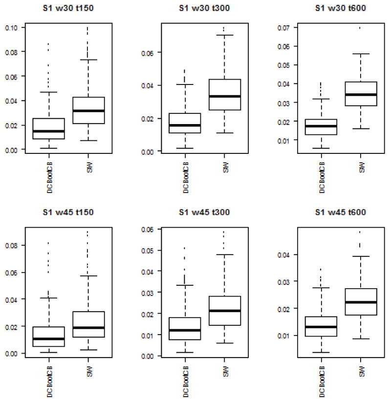
Boxplots of the MSE between estimated dFC and the true value of correlation for dFC calculated using DCBootCB algorithm and regular sliding-window technique for Scenario 1 - constant correlation across time.

Figure 7.

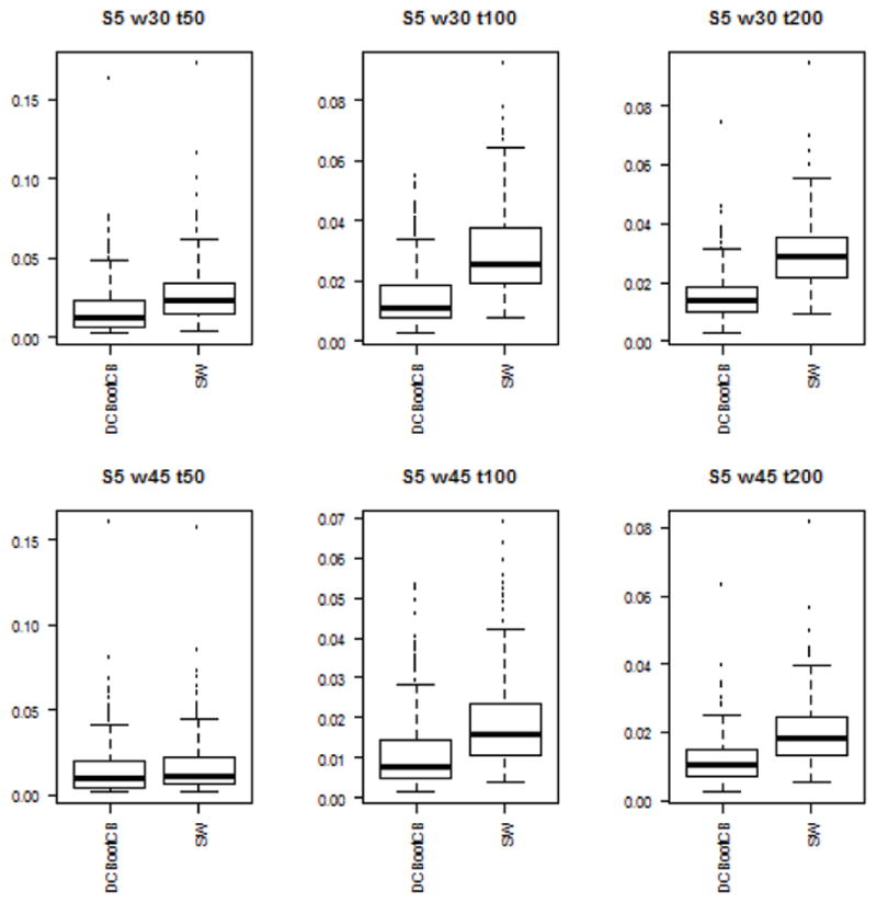
Boxplots of the MSE between estimated dFC and the true value of correlation for dFC calculated using DCBootCB algorithm and regular sliding-window technique for Scenario 5 - piecewise constant pyramid.

Summary

For the majority of the simulation scenarios considered, the DCBootCB method provides appropriate coverage of the true correlation function. The empirical coverage is very close to the nominal value. However, the proposed algorithm does not perform well in the case of step functions. This behavior was expected, as we are attempting to estimate the discontinuous function using smooth estimates. Fisher’s approximation does a better job in terms of coverage in the discontinuous correlation function case, at the cost of a significant increase in the width of the confidence interval. In addition, in Scenarios 1, 2 and 3, Fisher’s approximation gives an average coverage as great as 99.5%, illustrating that Fisher’s approximation tends to be overtly conservative.

5 Kirby 21 data application

We applied the DCBootCB algorithm to the “Multimodal MRI Reproducibility Resource” study [14], also known as the Kirby 21 dataset (http://www.nitrc.org/projects/multimodal). A detailed description of the study and data preprocessing steps can be found in Lindquist et al.[16]. Here, we use two repeated resting-state fMRI scans separated by a short break from 20 healthy adult volunteers. Each scan lasted 7 minutes resulting in 210 observations per subject per scanning session. Data was extracted from the six regions of interest defined in Chang and Glover [2], including the posterior cingulate cortex (PCC), the parietal cortex (Region 1), the frontal operculum (Region 2), the temporal cortex (Region 3), the orbitofrontal cortex (Region 4), and the anterior cingulate cortex (Region 5). The latter five regions were chosen due to the fact they showed high variability with the PCC during resting state. In Figure 8, we show examples of the original time series (left panels) and the dynamic connectivity estimates (right panels). The blue line depicts the estimate of dFC, the green line depicts the static correlation, and the red lines represent the confidence intervals. Specifically, we present the data from the PCC and the right interior frontal operculum for subject 2 during scan 2 and for subject 16 during scan 2, respectively. The dFC for subject 2 shows small changes across time, while the dFC for subject 16 shows higher variability across time. To summarize the dynamic behavior of FC for each subject, region, and scan, we calculated the non-static coverage, which is the percentage of time when the confidence interval does not contain the static correlation. When the CI covers the static correlation there is less evidence that the correlation coefficient changes dynamically over time. The results are shown in Figure 9 for each subject, region, and scan. The non-static coverage in Figure 9 exhibits high variability across subjects, regions, and scans, indicating that the assumption of a static correlation is not viable. In addition, we calculated the non-zero coverage(the proportion of the time points where the 95% CI does not contain zero), which indicates a significant association between two brain regions. Due to the dynamic nature of connectivity, the significance of association between two brain regions may vary across time. This property can be observed in Figure 10, where two heatmaps show the proportion of the non-zero coverage for each subject, region, and scan. For a number of pairwise associations, the value is high (dark blue) indicating that the assumption of a constant zero correlation is not appropriate. We also note high non-zero coverage variability across subjects, regions, and scans.

Figure 8.

Left panels show raw time series and right panels estimated dynamic correlations between the PCC and the right interior parietal cortex for subject 2 undergoing scan 2 (small changes in FC) and for subject 16 undergoing scan 2 (large changes in FC). The green line on the right panel represents the static correlation.

Figure 9.

The proportion of the time interval where the dynamic correlations 95% CI does not cover the static correlation between the PCC and 5 ROIs for each subject, region and scan.

Figure 10.

The proportion of the time interval where the dynamic correlations 95% CI does not cover the zero correlation between the PCC and 5 ROIs for each subject, region and scan.

As a further illustration, we present results from the second scan for subjects 2 and 16 (see Figures 9 and 10). For subject 2, the non-static coverage between the PCC and each of the five other regions implied by a 95% CI is equal to 0%. This implies that a static correlation is sufficient to describe their associations. In contrast, the non-zero coverage is on average equal to 56% and varies between 22.10% and 98.9%. For example, the non-zero coverage between PCC and the right inferior frontal operculum (ROI2) is 47% and between PCC and the right inferior orbitofrontal cortex (ROI4) is 98.9%.

For subject 16, the results were quite different. Here the non-static coverage is on average equal to 18.3% and varies between 0% and 56.9%. For example, the non-static coverage between PCC and the right inferior frontal operculum (ROI2) is 56.9% and between PCC and the right inferior orbitofrontal cortex (ROI4) is 15.5%. Hence, a static correlation is not sufficient to describe the association between these two particular brain regions. The nonzero coverage is on average equal to 23.6% and varies between 0% and 48.6%. For example, the non-zero coverage between PCC and the right inferior frontal operculum (ROI2) is 47.5% and between PCC and the right inferior orbitofrontal cortex (ROI4) is 48.6%.

Application of DCBootCB to the Kirby 21 data set demonstrates that the estimated dynamic correlation is extremely variable and that providing only point estimates of the correlation can be misleading. Uncertainty estimation enables us to decrease the chance of making false positive statements about either non-zero association or static behavior of the connectivity.

6 Discussion

The most common approach towards assessing the dynamic nature of FC has been the sliding-window technique. In this paper, we studied the properties of this method. Our main contribution was to introduce a method for obtaining non-parametric estimation of the confidence bands for the dynamically changing correlation coefficient. To do so, we utilized the MLPB method, which was designed specifically to generate valid bootstrap samples for multivariate correlated time series. We computed the confidence intervals to determine if there was evidence of a time-varying statistical association between two brain regions and to provide a summary measure of the degree to which it varies. To the best of our knowledge, such an approach has never been implemented in a study of connectivity using fMRI data.

The DCBootCB method requires specification of three tuning parameters: (1) the number of sampling points used for the correlation estimation; (2) the size of the smoothing window; and (3) the width of the adjacent blocks in the bootstrap algorithm. We based our choice of the sliding-window size on published empirical results. The most common width of the window was either 30 or 45 time points, and it has been shown that application of the much larger window length does not appropriately capture the dynamically changing signal. Similarly, the smoothing window size was selected to be 30 time points. The width of the adjacent blocks was equal to 30 time points in the bootstrap algorithm to guarantee the stability of the covariance matrix estimation. In future work, we will explore the effect of different block sizes.

In a series of simulation studies, we showed that the proposed confidence bands behave well. We considered situations of no association between the two time-series, gradually changing association, and step-wise constant association. Our simulation results lead us to conclude that the MLPB approach to bootstrapping correlated time series provides a valid model-free, time-varying connectivity estimates together with associated confidence bands. We showed that point estimates for the correlation coefficient alone are not sufficient to assess connectivity, and it is necessary to also include uncertainty measures. In addition, our simulation studies show that the theoretical results are supported by empirical evidence. It is expected that when the correlation goes up, the width of confidence intervals will get narrower.

We compared confidence bands obtained by the DCBootCB algorithm with the Fisher asymptotic results. The precision of coverage of a true correlation coefficient was much better for the DCBootCB algorithm. We found that the Fisher asymptotic approximation tends to overestimate the coverage of confidence bands for dynamically changing correlation. The proposed algorithm has some difficulties with discontinuous functions. This is illustrated in simulation Scenarios 4 and 5. The main problem appears on the boundaries between the step-wise constant pieces. Even though this is a limitation of the DCBootCB algorithm, in practice, resting state dynamic correlation tends to change gradually, which was mimicked in simulation Scenarios 2 and 3.

We applied the DCBootCB algorithm to the Kirby-21 resting state data. We focused on assessing dynamic correlation between the PCC located in the default-mode network, and 5 ROIs known from the literature to display a high degree of variability with the PCC across time. On the one hand, results obtained in the analysis of the Kirby-21 data confirmed the high variability between regions and subjects in the same scan. On the other hand, we found high variability between scans performed on the same subject casting doubt on the reproducibility of the intra-subject dynamic correlation patterns.

In conclusion, we addressed one of the main issues associated with applying the sliding-window technique to estimate functional connectivity – the lack of assessment of uncertainty. Unfortunately, much of the functional connectivity research is focused exclusively on the connectivity estimation without proper confidence band estimation. The introduced DCBootCB algorithm provides a mechanism to estimate the uncertainty using confidence bands that are not readily available in other cases. We also showed in a simulation study that the properties of the proposed algorithm are better in terms of coverage than Fisher’s asymptotic approach.

Figure 4.

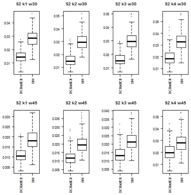
Boxplots of the MSE between estimated dFC and the true value of correlation for dFC calculated using DCBootCB algorithm and regular sliding-window technique for Scenario 2 - sine function.

Figure 5.

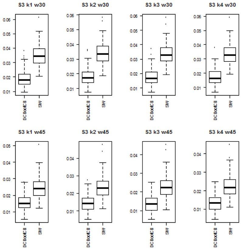
Boxplots of the MSE between estimated dFC and the true value of correlation for dFC calculated using DCBootCB algorithm and regular sliding-window technique for Scenario 3 - Gaussian kernel.

Figure 6.

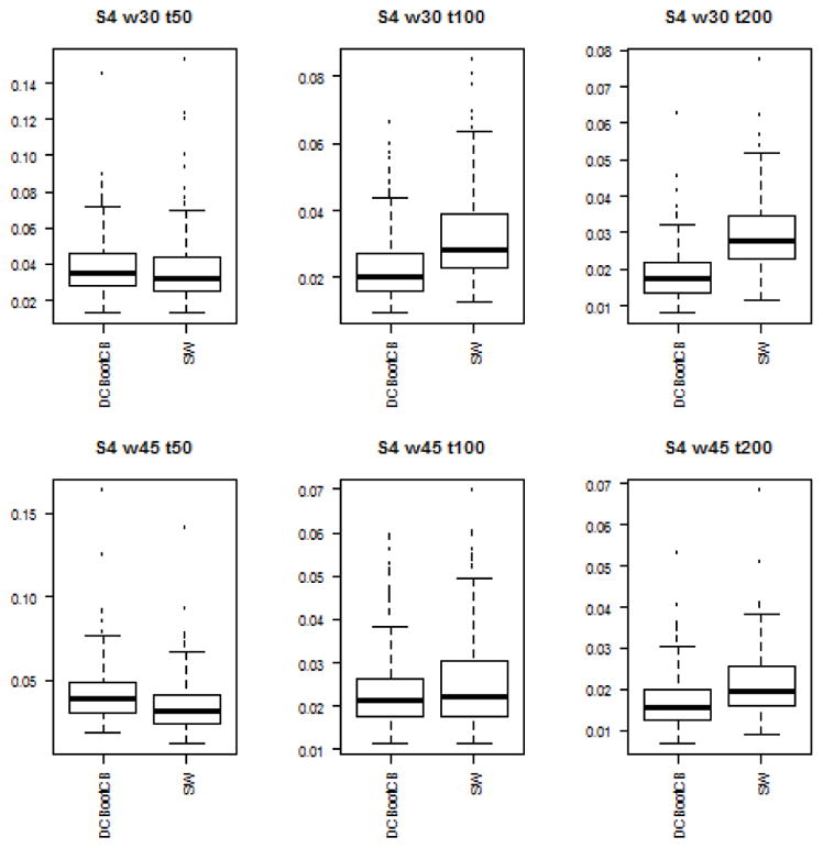
Boxplots of the MSE between estimated dFC and the true value of correlation for dFC calculated using DCBootCB algorithm and regular sliding-window technique for Scenario 4 - step-wise constant correlation across time.

References

- 1.Allen Elena A, Damaraju Eswar, Plis Sergey M, Erhardt Erik B, Eichele Tom, Calhoun Vince D. Tracking whole-brain connectivity dynamics in the resting state. Cerebral cortex. 2012:bhs352. doi: 10.1093/cercor/bhs352. [DOI] [PMC free article] [PubMed] [Google Scholar]
- 2.Chang Catie, Glover Gary H. Time–frequency dynamics of resting-state brain connectivity measured with fmri. Neuroimage. 2010;50(1):81–98. doi: 10.1016/j.neuroimage.2009.12.011. [DOI] [PMC free article] [PubMed] [Google Scholar]
- 3.Cribben Ivor, Haraldsdottir Ragnheidur, Atlas Lauren Y, Wager Tor D, Lindquist Martin A. Dynamic connectivity regression: determining state-related changes in brain connectivity. Neuroimage. 2012;61(4):907–920. doi: 10.1016/j.neuroimage.2012.03.070. [DOI] [PMC free article] [PubMed] [Google Scholar]
- 4.Cribben Ivor, Wager Tor D, Lindquist Martin A. Detecting functional connectivity change points for single-subject fmri data. Frontiers in computational neuroscience. 2013;7 doi: 10.3389/fncom.2013.00143. [DOI] [PMC free article] [PubMed] [Google Scholar]
- 5.Filippini Nicola, MacIntosh Bradley J, Hough Morgan G, Goodwin Guy M, Frisoni Giovanni B, Smith Stephen M, et al. Distinct patterns of brain activity in young carriers of the apoe-e4 allele. Proceedings of the National Academy of Sciences. 2009;106(17):7209–7214. doi: 10.1073/pnas.0811879106. [DOI] [PMC free article] [PubMed] [Google Scholar]
- 6.Friston Karl J. Functional and effective connectivity in neuroimaging: a synthesis. Human brain mapping. 1994;2(1–2):56–78. [Google Scholar]
- 7.Friston Karl J. Functional and effective connectivity: a review. Brain connectivity. 2011;1(1):13–36. doi: 10.1089/brain.2011.0008. [DOI] [PubMed] [Google Scholar]
- 8.Handwerker Daniel A, Roopchansingh Vinai, Gonzalez-Castillo Javier, Bandettini Peter A. Periodic changes in fmri connectivity. Neuroimage. 2012;63(3):1712–1719. doi: 10.1016/j.neuroimage.2012.06.078. [DOI] [PMC free article] [PubMed] [Google Scholar]
- 9.Hindriks Rikkert, Adhikari Mohit H, Murayama Yusuke, Ganzetti Marco, Mantini Dante, Logothetis Nikos K, Deco Gustavo. Can sliding-window correlations reveal dynamic functional connectivity in resting-state fmri? NeuroImage. 2016;127:242–256. doi: 10.1016/j.neuroimage.2015.11.055. [DOI] [PMC free article] [PubMed] [Google Scholar]
- 10.Matthew Hutchison R, Womelsdorf Thilo, Allen Elena A, Bandettini Peter A, Calhoun Vince D, Corbetta, et al. Dynamic functional connectivity: promise, issues, and interpretations. Neuroimage. 2013;80:360–378. doi: 10.1016/j.neuroimage.2013.05.079. [DOI] [PMC free article] [PubMed] [Google Scholar]
- 11.Jentsch Carsten, Politis Dimitris N, et al. Covariance matrix estimation and linear process bootstrap for multivariate time series of possibly increasing dimension. The Annals of Statistics. 2015;43(3):1117–1140. [Google Scholar]
- 12.Jones David T, Vemuri Prashanthi, Murphy Matthew C, Gunter Jeffrey L, Senjem Matthew L, Machulda, et al. Non-stationarity in the resting brains modular architecture. PloS one. 2012;7(6):e39731. doi: 10.1371/journal.pone.0039731. [DOI] [PMC free article] [PubMed] [Google Scholar]
- 13.Kreiss Jens-Peter, Paparoditis Efstathios. Bootstrap methods for dependent data: A review. Journal of the Korean Statistical Society. 2011;40(4):357–378. [Google Scholar]
- 14.Landman Bennett A, Huang Alan J, Gifford Aliya, Vikram Deepti S, Lim Issel Anne L, Farrell Jonathan AD, et al. Multi-parametric neuroimaging reproducibility: A 3-t resource study. NeuroImage. 2011;54(4):2854–2866. doi: 10.1016/j.neuroimage.2010.11.047. [DOI] [PMC free article] [PubMed] [Google Scholar]
- 15.Leonardi Nora, Van De Ville Dimitri. On spurious and real fluctuations of dynamic functional connectivity during rest. Neuroimage. 2015;104:430–436. doi: 10.1016/j.neuroimage.2014.09.007. [DOI] [PubMed] [Google Scholar]
- 16.Lindquist Martin A, Xu Yuting, Nebel Mary Beth, Caffo Brain S. Evaluating dynamic bivariate correlations in resting-state fmri: A comparison study and a new approach. NeuroImage. 2014;101:531–546. doi: 10.1016/j.neuroimage.2014.06.052. [DOI] [PMC free article] [PubMed] [Google Scholar]
- 17.McMurry Timothy L, Politis Dimitris N. Banded and tapered estimates for autocovariance matrices and the linear process bootstrap. Journal of Time Series Analysis. 2010;31(6):471–482. [Google Scholar]
- 18.Starck Tuomo, Nikkinen Juha, Rahko Jukka, Remes Jukka, Hurtig Tuula, Haapsamo Helena, et al. Resting state fmri reveals a default mode dissociation between retrosplenial and medial prefrontal subnetworks in asd despite motion scrubbing. Frontiers in human neuroscience. 2013;7 doi: 10.3389/fnhum.2013.00802. [DOI] [PMC free article] [PubMed] [Google Scholar]
- 19.Xu Yuting, Lindquist Martin A. Dynamic connectivity detection: an algorithm for determining functional connectivity change points in fmri data. Frontiers in neuroscience. 2015;9 doi: 10.3389/fnins.2015.00285. [DOI] [PMC free article] [PubMed] [Google Scholar]