A low-cost, scalable, current-sensing digital headstage for high channel count μECoG

Abstract

Objective

High channel count electrode arrays allow for the monitoring of large-scale neural activity at high spatial resolution. Implantable arrays featuring many recording sites require compact, high bandwidth front-end electronics. In the present study, we investigated the use of a small, light weight, and low cost digital current-sensing integrated circuit for acquiring cortical surface signals from a 61-channel micro-electrocorticographic (μECoG) array.

Approach

We recorded both acute and chronic μECoG signal from rat auditory cortex using our novel digital current-sensing headstage. For direct comparison, separate recordings were made in the same anesthetized preparations using an analog voltage headstage. A model of electrode impedance explained the transformation between current- and voltage-sensed signals, and was used to reconstruct cortical potential. We evaluated the digital headstage using several metrics of the baseline and response signals.

Main results

The digital current headstage recorded neural signal with similar spatiotemporal statistics and auditory frequency tuning compared to the voltage signal. The signal-to-noise ratio of auditory evoked responses (AERs) was significantly stronger in the current signal. Stimulus decoding based on true and reconstructed voltage signals were not significantly different. Recordings from an implanted system showed AERs that were detectable and decodable for 52 days. The reconstruction filter mitigated the thermal current noise of the electrode impedance and enhanced overall SNR.

Significance

We developed and validated a novel approach to headstage acquisition that used current-input circuits to independently digitize 61 channels of μECoG measurements of the cortical field. These low-cost circuits, intended to measure photo-currents in digital imaging, not only provided a signal representing the local cortical field with virtually the same sensitivity and specificity as a traditional voltage headstage but also resulted in a small, light headstage that can easily be scaled to record from hundreds of channels.

1. Introduction

With the growing use of high channel count multielectrode arrays in neural recordings [1–10] it is desirable that front-end electronics achieve a balance between high quality multichannel amplification and minimal headstage footprint. In addition, the ever-growing number of recording sites demands strategies for sharing multiple sources of information on a reduced number of communication channels. Analog (time-division) multiplexing has been a key element in multiple electrophysiology systems [3, 11–14], enabling the use of a single high quality analog to digital converter (ADC) among multiple electrode channels. The miniaturization of high rate ADCs with MHz bandwidth has allowed digitization of the multiplexed signal within the headstage circuit [15]. On-board digitization improves the recording fidelity as the serialized digital words are largely immune to transmission errors, setting the final signal-to-noise ratio (SNR) at the headstage level. A digital interface also shifts much of the burden of recording to the headstage electronics, which allows for simple, portable data acquisition (DAQ) electronics and promotes generalized interface software [16].

An alternative approach to digitizing a multiplexed signal would be to directly amplify and digitize multiple sources in parallel. To leverage existing solutions, we considered another class of sensing modalities, digital radiography, with sensor counts and signal throughput that far exceed modern electrophysiology [17, 18]. Digital radiography, like digital photography, replaces photo-sensitive film with a grid of photosensitive semiconductor elements such as charge-coupled devices (CCDs) or photo-diodes multiplexed through thin-film transistors (TFTs). Parallel, high speed digitization of the electronically transduced light levels is necessary to support short-latency imaging with mega-pixel dimensions. Additionally, the price per channel of imaging circuits is much lower than digital electrophysiology systems, due partly to mass production for medical and security scanners.

Transimpedance (current) amplifiers are commonly used in electrophysiology for measuring minute, localized currents such as in patch clamping [19] and amperometry [20]. When measuring extracellular fields, however, it is customary to use voltage amplifiers that have high input impedance (reducing the current in the electrode) rather than current amplifiers with virtually zero input impedance. It is well known with voltage-controlled neural stimulation that the electrode-electrolyte interface impedance creates a complex-valued load that transforms the resulting current in a time- and frequency-dependent manner [21, 22]. A voltage pulse must be pre-compensated to deliver the desired current pulse [23]. In the context of neural recordings, current at the electrode will transform the cortical potential signal in a frequency-dependent manner [24]. We found that the impedance transformation was well characterized and corrected by an invertible linear time-invariant filter model that recovered an accurate potential signal with improved signal to noise properties.

We introduce in the present study a novel approach to on-board digitization of neural signals that bypasses analog multiplexing altogether. We used a parallel, ultra-low noise current-sensing ADC incorporated in a commercially available integrated circuit (IC). The headstage provided a digital interface to a 61-channel flexible μECoG electrode array using a 2mm gauge micro high-definition multimedia interface (micro-HDMI) cable. The use of a single IC allowed for a very small-volume, low-mass headstage that is easily implantable, and multiple circuits can be chained together making it easily scalable for higher channel count systems. We validated the current-sensed neural signal from anesthetized rat auditory cortex by comparison with voltage-sensed signals from replicated recordings in the same animals. We also present results from an awake freely-moving animal implanted with a current-sensing system for 52 days. Although there was little difference in the stimulus related content of the current and voltage signals, we found that correcting for the electrode transformation had favorable signal-to-noise properties.

2. Methods

2.1. Headstage and electrode design

2.1.1. Digital current-sensing headstage

The current-sensing headstage was designed around a Texas Instruments (TI) DDC264 current-sensing ADC. The DDC circuit (Figure 1) measured electrical charge through transimpedance amplifiers with capacitive feedback (Figure 2, current-sensing amplifier), a configuration called an integrating amplifier since the voltage output is related to the integral of the current input

Figure 1.

Digital μECoG recording system. Cortical current sensed by a 61-channel flexible printed circuit board (flex-PCB) electrode was digitized at the headstage by a DDC 264 current-input, analog to digital converter from Texas Instruments (TI). The headstage interfaced with the electrode using a high-density, low-profile zero insertion force (ZIF) connector. Digital command and signal lines were carried by an ultra-flexible, 2 mm thick micro-HDMI cable. A translation stage was implemented on an ICE 40 FPGA (Lattice Semiconductor) to mimic the Intan RHD2000 series digital interface and interact with the Open Ephys acquisition system. Future updated software and hardware in the Open Ephys system would eliminate the need for an intermediate translation FPGA. (Open Ephys imagery used with permission.)

Figure 2.

The effect of electrode-electrolyte interface (EEI) impedance on transimpedance sensing. (a) The cortical potential field was measured through a current-sensing transimpedance amplifier (upper-right) and a voltage-sensing buffer amplifier (lower-right). The impedance of the EEI had virtually no effect on the potential at the input of the high-impedance voltage-sensing circuit. Conversely, the electrode caused a significant transformation on the potential at the input of the low input-impedance current-sensing circuit. The EEI was modeled as a simplified Randles circuit having finite and real DC impedance. (b) A model 1/f² LFP power spectrum in its natural current-sensed form is shaped by the squared-inverse of the impedance spectrum |Z(f)|⁻². The electrode impedance also generates thermal noise with power proportional to ℛ{Z⁻¹(f)}. Rebalancing the LFP and noise spectra using the electrode impedance simultaneously recreates the 1/f² LFP spectrum and decreases the noise power. Rebalancing the current-sensed signal also enhances the signal to noise ratio in the bandwidths corresponding to the 1/f capacitive effect of the electrode.

$$V_o(t)=V_{\mathit{off}}-\frac{1}{C_f}{\int }_0^t{I}_i(u)du.$$

The circuit accumulated charge over one sampling period and current was estimated as the net charge divided by the period. Each input channel used dual transimpedance amplifiers that alternated at each sampling period between integrating charge and buffering an output for digital quantization.

The parallel ADCs quantized at 20 bits with a maximum rate of 6 kS/s and average noise of 0.72 fC RMS (equivalent to 4.3 pA RMS for a 167 μs integration time). We mounted the 9.1×9.1 mm² DDC circuit on a 21×14 mm² printed circuit board mapping digital outputs to a μHDMI connector. Analog inputs were connected to a 61-channel flexible-PCB electrode [14] through a 61-pin zero insertion force (ZIF) connector (Figure 1). The total mass of the headstage was 1.4 g.

To interface with the Open Ephys acquisition system (www.open-ephys.org), we developed a front-end to back-end translation system on a field programmable gate array (ICE40 FPGA, Lattice Semiconductor). The translating FPGA mimicked the Intan RHD2000 series digital interface at the back-end, allowing the Open Ephys hardware to command and receive digital samples from the DDC headstage front-end. A custom PCB was also developed to adapt the FPGA IO to the HDMI front-end and SPI (Omnetics PZN-12) back-end cables, as well as to power the FPGA and DDC circuits.

2.1.2. Analog voltage headstage

The voltage-sensing headstage, previously described in [25] and [14], used analog multiplexing circuits (Analog Devices ADG726) to combine 60 electrode channels (excluding the unexposed electrode) into four analog channels. The multiplexed signals were then digitized at 250 kS/s by a National Instruments multicard PXI system with 18-bit ADCs. With an oversampling factor of 8 and 16:1 multiplexing, the final sampling rate per electrode channel was 1953 S/s.

2.1.3. Flexible μECoG electrode

Cortical fields were sensed by a 61-channel flexible printed circuit board (flex-PCB) μECoG electrode described previously in [26] and [14]. The 27 μm thick array was arranged as an 8×8 grid with three corners missing (the last corner contains an electrode left covered by the soldermask outer layer). Each contact was a 200 μm diameter disk of electroless nickel immersion gold finish, and the total brain recording area was 3.25×3.25 mm².

2.2. Surgical procedure for awake and anesthetized recordings

All animal procedures were performed in accordance with National Institutes of Health standards and were conducted under a protocol approved by the New York University School of Medicine Institutional Animal Care and Use Committee. Adult male Sprague-Dawley rats (n=3) were anesthetized with ketamine (40 mg/kg, intramuscular injection) and dexmedetomidine (0.125 mg/kg, intramuscular injection), and the head was secured in a custom head-mount that left the ears unobstructed. The skull was exposed with a longitudinal incision and five bone screws were inserted into the skull. After reflecting the right temporalis, a 5×5 mm² craniotomy was made, and a sterilized electrode array was placed subdurally over auditory cortex using vasculature landmarks. For the recovery procedure, the array was placed epidurally and the craniotomy was covered in a 1.5 percent solution of warm agarose. After the agarose solidified, the craniotomy was encapuslated in cement (Grip Cement, Dentsply Caulk). After the array was secured, silver wire was soldered between the headstage and bone screws to be used as ground and reference. Finally, the entire headstage was covered in cement and the animal was left to fully recover before electrophysiological recordings began.

2.3. Electrophysiological recording and stimulus presentation

Electrophysiological recordings were made in a sound-attenuation chamber. Responses to 50 ms tone pips of 13 frequencies (0.5–32 kHz, 0.5 octave spacing, 2 ms cosine-squared ramps, 70 dB SPL) were recorded at each electrode site. Tones were presented in a pseudorandom sequence at a rate of 1.25 Hz to the contralateral ear using a calibrated free-field speaker (MF1 Multi-Field Magnetic Speaker, Tucker-Davis Technologies). Analog voltage recordings were made at the maximum sampling rate of 1953 S/s. Digital current recordings were made at 5000 S/s.

2.3.1. Noise reference recordings

Reference recordings were made using one of two methods in order to measure the noise contributed by the combined electrode and headstage systems. In one setup, the electrode was placed in a bath of saline and the headstage ground was connected to the bath by a gold or silver wire, creating a closed circuit through the electrode. Reference recordings were also made in one of the acute preparations shortly after the animal had been euthanized.

2.4. Signal and noise effects of electrode-electrolyte impedance

Metals in contact with an electrolytic solution form a complex-valued, frequency-dependent impedance. In typical neural recording electronics, extracellular potential is buffered by active amplification in a non-inverting operational amplifier (e.g., the op-amp in unity-gain mode in Figure 2(a). With a sufficiently high amplifier input impedance that exceeds the electrode impedance by several orders of magnitude, very little current moves into or out of the amplifier and the potentials on both sides of the electrode are virtually equal [24].

By contrast, the current-input ADC amplifiers have transimpedance configuration that maintains a virtual reference potential at the input terminals. As a consequence, the entire potential difference between the electrode and the reference is “dropped” as current across the electrode, transforming the potential signal in the process. The frequency dependent relationship between the true cortical potential and the sensed current is given by Ohm’s law: V_c(f) = I_in(f)Z_e(f).

We adopted a simplified Randles equivalent circuit model of electrode impedance that includes a capacitance C_dl representing the reactance of the electrical double layer and a resistance R_ct capturing the ability to pass Faradaic current through redox reactions [21]. A series resistance R_s includes the impedance of the tissue between the recording electrode and a reference electrode, which is (to a good approximation) real valued [27, 28]. (Due to its large size, the reference electrode’s impedance was assumed to be much lower than the μECoG electrode and was excluded from the model.) The transfer function of this equivalent circuit model is

$$Z(s)=\frac{s(R_s{R}_{ct}{C}_{dl})+R_s+R_{ct}}{s(R_{ct}{C}_{dl})+1}.$$ (1)

Figure 2(a) depicts an electrode impedance model using circuit values obtained from in vivo electrode impedance spectroscopy of a flex-PCB electrode made in a separate experiment.

A second consequence of the current-input circuit is its sensitivity to thermal noise generated by the electrode impedance [29–31]. The frequency distribution of thermally generated current in an impedance element is proportional to the real part admittance (conductance). In the case of electrode impedance modeled by Eq 1, the DC noise level proportional to (R_s+R_ct)⁻¹ will rise with frequency until it reaches a level proportional to $R_s^{-1}$.

The effects of electrode impedance on a “1/f” local field potential (LFP) power spectrum [32, 33] are illustrated in Figure 2(b). An LFP spectrum proportional to [1+(f/f₀)²]⁻¹ has been shaped by an impedance transfer function, which is the squared inverse of the spectrum in Figure 2(a), to form the power spectrum of the current-sensed field. The current spectrum has been scaled to match the actual variance of recorded current signals; the potential spectrum is presented on the same scale for clarity. On the same plot, we show the theoretical noise spectrum of the Randles circuit at a rat’s temperature of 37 °C. At higher frequencies, the power of the thermal noise reaches the power of the model cortical signal, with deleterious effects on the SNR integrated to large bandwidths (Figure 2(b), right).

2.4.1. Signal conditioning based on impedance transformation

If the Fourier transform of the impedance spectrum [ℱ⁻¹Z_e] (t) exists, then a reconstruction of the pre-electrode potential can be recovered by convolving this function with the measured current: v^(r) = i^(m) * z_e. Although such a transformation would attenuate the current signal, SNR properties would be enhanced (note, for example, the rebalanced signal, noise and SNR spectra in Figure 2(b) as well as the theoretical justification in Appendix Appendix A). To obtain an impedance spectrum that is absolutely integrable, we used the simplified Randles equivalent circuit of Eq 1. By using real-valued resistance in parallel with a true capacitive element, the model electrode has a rational frequency response that can be efficiently implemented as an order-one infinite impulse response (IIR) filter.

We estimated the values of the circuit elements by expressing the magnitude impedance in terms of a transfer function that related the power spectral densities of the current and voltage recordings: S_v(f)/S_i(f) = |Z_e(f)|². Although the two signals were not recorded simultaneously, we assumed that the average power of the cortical potential did not change over the course of the experiments. All spectra were resampled onto a log-constant frequency grid to avoid over-fitting higher frequencies, and circuit elements were found on a site-by-site basis to optimize the squared-error loss between the model impedance magnitude and the square root of the ratio of power spectra. Optimization was performed by the Levenberg-Marquadt method implemented in the Scientific Python library [34]. Impedance filters were then screened for irregular fits yielding a pole less than 0.1 Hz or a zero less than 1 Hz, whereupon the pole and zero were replaced with local median values. See Supplemental Figure 1 for examples of measured spectral ratios and the impedance spectra of the model circuit. Goodness of fit was measured by the fraction of variance unexplained (FVU), which is the ratio of the variance of the model’s residual to that of the raw spectrum. Variances were measured under the logarithm, to better represent a dynamic range of multiple orders of magnitude.

2.5. Neural signal analysis

2.5.1. Bandpass and impedance filters

The measured signals from each device (current and voltage) were filtered offline in order to reconstruct an estimate of the complementary signal. Digital impedance filters were formed from the estimated analog impedance filters by the bilinear transform method of frequency-warping $s\to 2f_s\frac{1-z^{-1}}{1+z^{-1}}$, where f_s is the sampling frequency of the signal to be transformed [35]. Subsequent bandpass filtering was performed offline using 6th order zero-phase digital Butterworth filters.

2.5.2. Spectral analysis

All power spectral densities (PSDs) were estimated using Thomson’s multitaper method derived from an orthonormal set of signal tapers {v_k(N,NW)} called Slepian functions that optimally span a lowpass subspace of (digital) bandwidth 2W in N-dimensional signal space [36, 37]. Uncorrelated spectral coefficients were computed with a limited number of tapers (K ≤ 2NW − 1) and averaged to find a final spectral estimator Ŝ_x(f):

$$\begin{array}{l}{y}_k(f)=\sum _{t}x(t)v_k(t)e^{-i2\pi ft}\\ {\widehat{S}}_x(f)=\frac{1}{K}\sum _{k=1}^K{\mid y_k(f)\mid }^2.\end{array}$$ (2)

A bandwidth resolution of 2W = 1 Hz and window size of 10 seconds was used for all spectra. To further reduce variance, spectral estimates were averaged over non-overlapping blocks of recording. In some recordings, line-noise artifacts were removed by linear interpolation in a ±W frequency window around the spectral line. Frequency-indexed signal-to-noise ratios (SNRs) were defined in both a frequency-resolved manner by taking the point-by-point ratio of physiological and noise PSDs, and a bandpass manner by finding the ratio of cumulative power at frequency f in the physiological and noise PSDs respectively.

High resolution spectrograms were estimated by computing complex-demodulates of signal strips analyzed by Eq 2 [38, 39]. The time-frequency function was composed by expanding the spectral coefficients y_k(f) onto the baseband signal space spanned by the Slepian functions

$$s(t,f)={\left|\sum _k{v}_k(t)y_k(f)\right|}^2.$$

A window size of 100 ms was used with a bandwidth 2W = 100 Hz. Complex demodulates were computed for overlapping windows staggered by 5 ms, and magnitudes were averaged to form the full spectrogram.

2.5.3. Spatial covariance

We organized measurements of the spatial random field x(s) using the semivariogram function, which reflects the variance of the difference between electrode signals as a function of distance

$$\gamma (h)=\frac{1}{2}\mathit{var}\{x_s-x_{s-h}\}=C_x(0)-C_x(h)$$ (3)

where C_x is the spatial covariance function of x. We modeled the random field as a mixture of two components. A spatially varying component η had covariance described by the Matérn function

$$C^{(m)}(h)\propto {(h/\theta )}^{\nu }{\mathcal{K}}_{\nu }(h/\theta )$$

where 𝒦_ν is the modified Bessel function of the second kind with order ν [40, 41]. The Matérn function is normalized to decrease from one to zero monotonically with distance. The spatial scale θ acts as a characteristic length, and the unit-less shape parameter ν controls the smoothness, or predictability, of the field within a radius of θ. As ν → 0, the covariance function corresponds to spatially white noise (C(h) ∝ δ(h)) and as ν → ∞, the covariance is Gaussian. A value of ν = 0.5 corresponds to an exponential covariance function [14, 42].

Additionally, we included a lumped process z for spatially homogeneous components with variance κ (e.g. line noise or other common artifact, and widely distributed electrophysiological rhythms). The process z only affects the marginal signal variance C_x(0) = C_η(0) + κ. Thus, the semivariogram (Eq 3) converges to zero variance for small spatial separations. However, since the component is spatially homogeneous (var{z_s − z_s−h} ≈ 0), the semivariance of the difference between signals at a large distance is less than the theoretical maximum of C_x(0) (the marginal variance).

The empirical semivariogram was computed by normalizing channels to have unit-variance and averaging the semivariance between all pairwise combinations of electrode sites at each possible lag h: 𝒟_h = {i, j : ||s_i − s_j|| = h}

$$\widehat{\gamma }(h)=\frac{1}{2\mid {\mathcal{D}}_h\mid }\sum _{i,j\in {\mathcal{D}}_h}{\langle {\mid x_i-x_j\mid }^2\rangle }_t$$

where 〈·〉_t indicates expectation over short blocks of time. To minimize serial correlations of the semivariance, signals were first whitened per channel with an autoregressive model. The asymptotic value of 1 − κ was estimated by the 98th percentile of the empirical semivariogram, and the model γ(h;Θ) = (1 − κ) [1 − C^(m)(h;Θ)] was optimized for Θ = {θ, ν} using the Levenberg-Marquadt method with iteratively defined residual weights equal to w_h = |𝒟_h|/γ(h;Θ) [43]. The full model of covariance for the field x(s) was

$${\widehat{C}}_x(h)=(1-\kappa )C^{(m)}(h;\mathbf{\Theta })+\kappa h>0.$$

Confidence intervals for parameters were inferred by performing 1000 estimations for bootstrap resampled pairwise semivariance. The spatial power spectrum of the random field η in one dimension was calculated from the Fourier transform of the Matérn covariance

$$f_{\eta }(k)\propto {\left[{\theta }^{-2}+{(2\pi k)}^2\right]}^{-\nu -\frac{1}{2}}.$$

Spatial half-band width k_B was defined as the −20 dB point in the spatial power spectrum. The corresponding critical sampling density was determined by the inverse of the full bandwidth Δ_x = (2k_B)⁻¹.

2.5.4. Evoked-response scoring

Middle-latency tone-evoked responses were windowed to a 50 ms post-tone period and each length-M response vector was scored by its Mahalanobis distance (MD) from a sample of baseline (unstimulated ECoG). The mean μ and covariance Σ were estimated from the baseline sample, taking care to regularize the generally ill-conditioned Σ through convex mixture of the sample covariance matrix with the identity [44]. The MD of an evoked response r is defined as

$$d^2(r)={(r-\mu )}^T{\mathrm{\sum }}^{-1}(r-\mu ).$$

An electrode’s best frequency was operationally defined as the tone frequency that evoked the largest mass of MD scores. The evoked signal-to-noise ratio (ESNR) was previously defined [14] by normalizing the square of the average best frequency MD score by the average squared self-distance of the baseline samples.

An important property of the MD is that it is invariant to any invertible (finite) linear transformation of the samples. Therefore, the MD based ESNR is (approximately) invariant to the impedance IIR filter.

To determine whether a site was responsive to tones, we computed Hotelling’s T² statistic [45] comparing the 30×13 (trials × tones) matrix of MD scores to a matrix of pseudo-scores computed on inter-stimulus signal. A site was deemed responsive at the p < 0.01 level.

2.5.5. Coregistration of array placement

We corrected for displacement between electrode positions by seeking a geometric transformation of the sensor locations that would maximize the cross-correlation of the 13-dimensional spatial fields derived from the average MD of evoked-responses to auditory tones. Holding the voltage-sensed recording fixed, a rotation and two-dimensional displacement of the current-sensed recording were found to maximize the sum of cross-correlations for all 13 response fields.

2.5.6. Tone classification

To predict the frequency of stimulation tones, we employed a supervised linear classifier based on the linear discriminants of compressed neural timeseries [46–48]. The method is described in detail in [14]. In brief, we formed feature vectors from concatenating the length-M post-tone timeseries of P responsive sites for each of N = 390 trials (13 frequencies × 30 repetitions). Singular value decomposition (SVD) was used to compress the feature vectors to an optimal rank R ≤ N (discovered through a cross-validated grid search), and linear discriminant analysis (LDA) was used to maximally separate the R-dimensional samples in a 12-dimensional projection. The classifier pipeline was implemented with the scikit-learn Python library [49].

Decoder results were tabulated in a normalized confusion matrix H_i,j representing the proportion of decoder predictions of frequency j given true stimulation with frequency i. In addition to accuracy ( $\frac{1}{13}\text{tr}H$), we computed the prediction error representing the average size of the misclassification in octaves:

$$e=\frac{1}{13}\sum _{i,j}\frac{1}{2}{H}_{i,j}\mid i-j\mid .$$

Accuracy and error values were bootstrapped by computing 10000 replicate confusion matrices formed by sampling decoder output with replacement within each class. We used generalized linear models to compare decode performance across different factors. Logistic regression was used to model prediction accuracy. Trial-by-trial decode errors take on discrete values and tend to be more dispersed for higher average error. Therefore, Poisson regression was used to model magnitude decoding error. The likelihood ratio test (LRT) was used to assess statistical significance of model factors relative to simplified models. Model results were adjusted for overdispersion by scaling relative to the Pearson χ² statistic of the simplified model [50]. Generalized linear models were implemented using the StatsModels library in Python [51]

3. Results

3.1. Neural recordings and impedance estimation

Stimulus-evoked responses were recorded on 108/120 sites (90%) using the current-sensing headstage, and 114/120 sites (95%) using the voltage-sensing headstage in two acute preparations. Figure 3 displays 1.5 second segments of μECoG recorded with either the current (Figure 3(a)) or voltage (Figure 3(b)) headstage. In both recordings, strongly evoked activity was observed in locations that varied with tone frequency. Normalized spectrograms of best frequency responses from an electrode with similar low-frequency tuning (Figure 3(c,d)) show that both signals followed similar time-frequency distributions, and that the current sensing headstage recorded larger response-to-background contrast at higher frequencies (Figure 3(e,f)).

Figure 3.

μECoG recorded from two headstages. Current (a) and voltage (b) signals from the same 8 electrode sites are shown during the same 1.5 second window in the auditory stimulation sequence. Tone presentation periods are marked in color below the time axis. Timeseries were bandpass filtered from 2–300 Hz. Auditory evoked responses on the scale of nano-amps were sensed with the digital headstage. The time course of the current responses resembled the first derivative in time of the cortical potential, due to the mainly capacitive nature of the electrode impedance in this bandpass. (c–f) The time-frequency distribution of response power from a similarly tuned electrode site showed high response-to-background contrast over a larger band of frequencies in the current-sensed signal. (c–d) Auditory tuning curves formed by the Mahalanobis distance of the current and voltage responses at site (3, 4). (e–f) Spectrograms of the 2 kHz auditory evoked responses (i.e.. shaded segments in (a–b)) from the current and voltage signals.

Power spectral densities confirmed the predicted increase in thermal noise due to the frequency-dependent electrode impedance (Figure 4). The noise floor of the current signal increased monotonically with frequency after ~ 10 Hz and intercepted the power level of the physiological signal at frequencies > 600 Hz. (The power spike at the Nyquist frequency of 2.5 kHz was due to offsets between the alternating samples from dual transimpedance amplifiers for each channel).

Figure 4.

Spectral content of measured and reconstructed signals. (a) The PSDs of the current-based recordings are shown as measured (solid, left ordinate) and as reconstructed (dashed, right ordinate). The gray spectra were calculated from noise recordings that included instrumentation noise and thermal noise from the electrode. Due to thermal noise, current noise increased with frequency. (b) PSDs of voltage-based recordings: as measured (solid, left ordinate), and as reconstructed (dashed, right ordinate). (Note that reconstructed amplitudes are only estimated in (a–b)). (c) Frequency-by-frequency SNR was calculated as the ratio of physiological and noise spectra. Only SNR of the measured signals are presented (the reconstructed SNR is mathematically identical). (d) SNR as a function of integrated band power. While the current-based signal had a larger gap between physiological and noise spectra in bands of physiological interest, the rising noise floor quickly diminishes wide-band SNR. Applying the voltage-reconstructing transform greatly mitigated the decline in SNR. (e) Integrated SNR of signals in common LFP bands: δ 1–4 Hz; θ 4–8 Hz; β 12–30 Hz; γ 30–100 Hz; high frequency included 100–950 Hz. The current based signal had significantly higher SNR in bands above δ, but only reconstructed voltage was significantly higher in the 100–950 Hz band. Conversely, reconstructed current had lower SNR above the β band. (Tukey’s honest significant difference test was performed for 1-way ANOVAs significant at p < 0.05).

The impedance transfer function model represented the ratio of voltage to current PSDs with very low error (Table 1 and Supplemental Figure 1). PSDs of reconstructed voltage and current signals closely matched their measured counterparts (by design). Similarly, the SNR-by-bandwidth measure of the current-sensed signal was greatly enhanced after correcting for the impedance transformation (as predicted, comparing Figures 4(d) and 2(b)). See Supplemental Figure 2 comparing timeseries from all measured and reconstructed signals.

Table 1.

Modified Randles Circuit Parameters (mean ± SEM) FVU: fraction of variance unexplained by model.

	Rct (MΩ)	Rs (kΩ)	Cdl (nF)	FVU
E1	10.0 ± 0.67	121 ± 10.0	20.5 ± 1.52	0.01 ± 0.00
E2	18.1 ± 1.76	211 ± 39.1	6.38 ± 0.47	0.02 ± 0.01

We also measured total SNR in common LFP bands (Figure 4(e)) and found that the current-based signal maintained a significantly higher sensitivity in beta and gamma bands (p < 0.001 Tukey’s HSD). However, only the impedance-corrected current signal maintained a significantly higher SNR for the 100–950 Hz band (p < 0.001). The estimated current signal, created by inverse-impedance filtering the voltage recording, showed degraded sensitivity in the gamma band and higher (p < 0.05).

3.1.1. Covariance of the random field

As a complementary analysis to the timeseries statistics, we analyzed the spatial random field of the two types of signals. Unlike the temporal nature of the signal, we did not anticipate that the electrode impedance should affect the spatial distribution. We compared models of spatial covariance fit to empirical semivariograms calculated from non-stimulated sections of 10–100 Hz bandpass signals (Figure 5). The model included a constant component accounting for spatially homogeneous processes that would reduce the asymptotic error between signals at long distances. The spatially varying component was modeled by the two-parameter Matérn covariance function.

Figure 5.

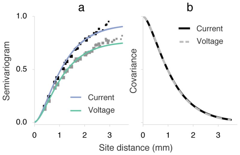
Spatial covariance of the current and voltage signals. (a) Empirical semivariograms (black squares: current; gray squares: voltage) indicate one half the mean squared-error difference between signals as a function of distance. Small values at short distances represent very little difference between signals. The theoretical maximum, equal to the overall signal variance, was normalized to unity. The size of squares corresponds to the mass of electrode pairs found at a distance. The semivariance model combined spatially varying and homogeneous field components. The lower asymptotic value of the voltage semivariogram indicated a larger proportion of the spatially homogeneous component. (b) The estimated Matérn covariance model (i.e. shared variance between sites) of the spatially varying components are shown, rescaled from 0–1. The two covariance functions are virtually identical between signals, suggesting that the random field was consistently measured with both modalities. The critical sampling density for this random field was estimated to be roughly 560 μm.

The empirical semivariograms portrayed spatial fields with distinct properties. In particular, only 7% of current signal variance was accounted for by spatially redundant signal power, compared with 23% for voltage (indicated by the parameter κ). In other words, a greater share of the voltage signal was approximately constant in space, indicated by a lower apparent asymptote for semivariance (Figure 5(a)). The spatially varying process, while accounting for different proportions of the signal variance, was consistent between the recordings. The Matérn function parameters, estimated through bootstrap resampling of the semivariance pairs, were virtually identical (Table 2, Figure 5(b)). The half-band widths k_B of Fourier transforms of the bootstrapped Matérn covariance estimates suggests critical sampling densities between 539–578 μm for voltage and 536–589 μm for current.

Table 2.

Matérn function parameters: bootstrapped median and 95% confidence interval.

Signal	θ (mm)	ν (unitless)	κ	FVU
i(t)	0.65 (0.64, 0.77)	1.03 (1.01, 1.32)	0.07	0.22
v(t)	0.65 (0.64, 0.73)	1.08 (1.06, 1.28)	0.23	0.30

3.2. Auditory coding of the evoked responses

We compared the sensitivity of each headstage to auditory cortical stimulus encoding by measuring the similarity in the spatial fields of evoked responses. Electrode placement-replacement error was corrected by a three-parameter coregistration described in Section 2.5.5. We found that the current and voltage signals capture essentially similar neural coding. After spatial alignment to account for electrode movement as depicted in Figure 6(a), the average cross-correlation of the tuning curves over 13 tones was 0.90.

Figure 6.

Reconstruction of evoked potential signals. (a) Tonotopic maps from voltage and current recordings. To compare the reconstruction quality from separate electrode placements in the same animal, the voltage and current recording grids were aligned to maximize the total cross-correlation of the frequency tuning spatial fields. The two frames indicate the estimated shift in array coverage from the voltage recording (solid frame) to the current recording (dashed frame). Following alignment, the average cross-correlation between tuning curves was 0.90. (b) Average best-frequency evoked responses are shown for all signal forms at the site with minimum voltage reconstruction error (0.69%). (c) Correlation coefficients for current (median 0.75) and voltage (median 0.98) suggested accurate reconstructions of response waveform shapes. (d) Reconstruction errors for current (median 29.1%) and voltage (median 11.1%) signals indicated parity of the overall response amplitudes.

Using the same array alignment, we assessed the effect of the impedance transform in terms of evoked-response waveform similarity. While the distribution of power by frequency over long periods was matched by design in the current-to-voltage reconstruction (and vice-versa), we also found that transient evoked responses were accurately reconstructed. Figure 6(b) depicts voltage- and current-domain average best-frequency responses for the coregistered array sites having minimum voltage reconstruction error, defined as ε = 100||v_m − v_r||²/||v_m||². The high normalized correlation between reconstructions (voltage median: 0.98, current median: 0.75) indicated recovery of the appropriate waveform shape, while the low reconstruction error (voltage median: 11.1%, current median: 29.1%) also indicated correct estimation of the amplitudes (Figure 6(c)).

The second anesthetized recording had a larger placement difference with linear translation distances between 1–2 electrode spacings. The tuning field correlation in this case was 0.72, and median voltage reconstruction error and correlation were 22.6% and 0.96, respectively.

3.3. Evoked response signal-to-noise

We measured evoked response SNR (ESNR) for responsive sites over the 2–300 Hz bandpass (Figure 7(a)). The current-sensing headstage provided a significantly higher ratio of evoked response energy to average background energy (t = 3.55, p < 0.001, paired Student’s t-test for N = 105 electrode sites). Similarly, the reconstructed voltage signal improved ESNR beyond the measured current signal (t = 13.5, p < 0.001, paired Student’s t-test), while the reconstructed current ESNR deteriorated relative to the measured voltage (t = −15.1, p < 0.001, paired Student’s t-test). The ESNR values of both signals were consistent with results from previous acute experiments [14]. Example best-frequency responses of sites scoring at 20th and 80th percentiles of ESNR are shown in Figure 7(a). The most immediate difference between recordings is the relatively low amplitude and narrow distribution of current baseline signal. We compared the distributions of baseline signal at matched electrodes and found the current baseline was significantly more peaked, with a median excess kurtosis of 4.7, than the distribution of voltage baseline, with a median excess kurtosis of 0.52 (W = 296, p < 0.001 Wilcoxon signed-rank test).

Figure 7.

Evoked SNR (ESNR) measured the statistical divergence of response signal from the inter-stimulus baseline signal for 105 matched electrode sites (53 and 52 electrodes from two rats). (a) Distributions of ESNR over a wide band (2–300 Hz) showed greater response sensitivity in the current based signal, with a further enhancement in the reconstructed voltage signal. Example evoked responses at best frequency were drawn from recording sites scoring at the 20th and 80th percentile of ESNR for both measured signals. (b) ESNR was computed in 40 Hz bands between 0 and 900 Hz (mean: solid traces; S.E.M.: margins). Lines were broken where the median ESNR was not significantly greater than a controlled SNR measured from baseline windows (Mann-Whitney U tests per frequency with false discovery rate limited to 0.05). Both recording devices were sensitive to evoked power over a large band, and the current signal was most sensitive for every band except the last (860–900 Hz). (For narrowband signal, ESNR was virtually equal between measured and reconstructed data; only raw data ESNR is shown.)

We computed a frequency-resolved comparison of ESNR on 40 Hz bandpasses centered between 20 Hz and 880 Hz in 30 steps (Figure 7(b)). The current-sensing headstage had improved ESNR at every bandpass except 860–900 Hz (p < 0.05, paired Student’s t-test with Bonferroni correction for 30 tests), including a plateau of high sensitivity extending ^~300 Hz greater than the voltage-sensing headstage. In the narrowband sense, the ESNR of reconstructed signals was virtually identical to that of measured signals due to similar proportions of thermal noise and the approximate invariance of the Mahalanobis distance to IIR filtering.

3.4. Decoding

We trained a linear classifier to decode tone frequency from neural responses in the 2–600 Hz bandpass. All signals yielded accuracy and error that outperformed the uniform chance levels of 7.69% and 2.15 octaves, respectively (Figure 8). The uncorrected current produced decoding with less accuracy and precision than the voltage based decoding, possibly due to higher proportions of measurement noise, Figure 4(d). Once the impedance correction was applied to reconstruct a voltage signal, decoding accuracy and error were indistinguishable from the original voltage decoding (χ₁ = 1.42, p = 0.23, LRT of logistical regressions, χ₁ = 2.34, p = 0.13, LRT of Poisson regressions, 8(b)). It should be noted that the decoding metrics of each signal met or exceeded the average accuracy of 52% and error of 0.53 octaves expected for a subdural ketamine preparation in rat auditory cortex [14].

Figure 8.

Error and accuracy for predicting 13 tones over 790 trials (390 trials classified separately each of 2 rats). (a) Confusion matrices pooled over two experiments show predictions highly concentrated along the diagonal, displaying a large proportion of correct and nearly correct classifications. (b) For all signals, measures of decoder error (left) and accuracy (right) were very distinct from chance levels (2.15 octaves and 7.69%, respectively). Transforming current to voltage improved the accuracy and error to levels indistinguishable from the measured voltage signal. Conference intervals of accuracy and error were estimated from 10000 bootstrap replicates of confusion matrices. Statistical inference was based on generalized linear models of the influence of signal type on decoder output (see Methods).

3.5. Chronic recordings

We implanted one rat with a 61 channel flex-PCB electrode connected to a current headstage, making five recordings over the course of 52 days. After this point the tone-evoked responses were no longer decodable beyond the level of uniform chance. Figure 9(a) shows normalized and averaged evoked responses at the best frequency of an example site. Evoked SNR was level at a median of 1.37 dB for the first 28 days (Figure 9(c)), and at all days was significantly greater than a control value measured with pre-stimulus windows (p < 0.05 paired Student’s t-test with Bonferroni correction for 5 tests). Tone frequency was decoded from the awake current recordings at 18.5% average accuracy (7.69% chance) and 1.55 octaves average error (2.15 octaves chance, Figure 9(d)).

Figure 9.

Evoked response waveforms and statistics over 52 days of an implanted current headstage. (a) Evoked responses of “raw” current recordings and signals conditioned with a lowpass impedance filter emphasizing electrode capacitance. The signal amplitude from each recording was normalized to have unit variance. Vertical bars indicate the time of tone presentation and span ±σ. (b) RMS current decreased appreciably over the course of the implant, likely reflecting rising electrode impedance. Mean RMS current on day 9 was 160 pA; by day 52 RMS current was bimodal with mean RMS current of 87.4 pA and 9.02 pA within each cluster of sites. The grayscale of sites is ordered by RMS current on day 9. (c) Evoked SNR levels were consistent with previous flex-PCB implants, but degraded by the later recordings. Circles and error bars indicate means and standard deviations over channels for each recording day. ESNR of the conditioned signal was significantly higher when controlling for varying levels per day. (d) Decoding accuracy and error were better than uniform chance and also degraded over the lifetime of the implant, consistent with previous flex-PCB results. Circles and error bars indicate means and 95% confidence intervals derived from bootstrapped samples of the decoder output. Dashed lines are logistic regressions of accuracy and Poisson regressions of error. Conditioning the signal was only a significant factor in the model of accuracy.

Given the improvements in ESNR and decoding seen in the anesthetized data when making an impedance transform, we attempted a similar conditioning of the awake data. Lacking an estimate of the electrode impedance spectrum, we made a simplification of Eq 1 having the form H(s) = (1+s/2πf₀)⁻¹. This system preserved the 1/s capacitor characteristic and finite DC impedance of the original model. We chose a corner frequency of f₀ = 15 Hz, which demonstrated improved response sensitivity and decoding performance. Although the conditioning filter was formally equivalent to an additional lowpass filter, it led to a significant increase in evoked SNR independent of the per-day variation (χ₁ = 6.11, p < 0.05, LRT, Figure 9(c)). Signal conditioning also led to significantly higher decoder accuracy (Figure 9(d)), independent of a regression over implant duration (χ₁ = 4.58, p < 0.05, LRT). However, the apparent decrease in decoder error was not significant in a Poisson regression of decoder error over implant duration (χ₁ = 3.71, p = 0.054, LRT).

By day 52, the RMS current level in the 2–100 Hz bandpass had lowered considerably from levels observed one week after implantation. 70% of sites (43 sites) had, on average, a 45% reduction in signal power. Signal power on the remaining 18 sites was reduced by 95%, likely due to a radical increase of electrode impedance related to metal corrosion of electrode sites and interconnects (Figure 9(b)). The divergence of signal power among these electrode sites appeared to begin after the 28th day of recording, consistent with in-vitro findings [52].

4. Discussion

We presented a digital headstage designed for μECoG recordings based on highly integrated charge-integrating amplifiers (Texas Instruments DDC264). The commercially available circuit was built for parallel readout of photo-currents in imaging systems with millions of sensors. By adapting the circuit for electrophysiology, we were able to independently amplify and digitize 61 channels of cortical current with a sampling rate sufficient for typical LFP bands as well as high-gamma and broadband activity. The capability of lightweight imaging circuits to digitize a large number of channels in parallel is a potent, scalable resource for developing compact, implantable headstage electronics able to acquire hundreds of electrode sites, or that can be used with small animals such as mice and gerbils. Although the use of current-input amplifiers is unconventional for extracellular field recordings, we demonstrated the compatibility of the current signal with voltage signals recorded in the same animals.

In all measures of signal content, the current-sensed signal represented the spatial and temporal dynamics of the cortical electric field in a virtually equivalent manner as the voltage-sensed signal. Auditory frequency-tuning curves, determined from evoked responses having different temporal shape, nonetheless had high average cross-correlation between recordings after correcting for alignment (ρ = 0.90 and ρ = 0.72 in two animals). As seen in Figure 6, the tonotopic maps built from the center of mass of electrode tuning curves were visually very similar. The two sensing modalities also appeared to equally represent the distribution of baseline signal power over varying spatial scales. Our model of the locally varying spatial random field covariance was indistinguishable between the two signals (Figure 5).

The digital headstage showed comparable or improved performance in measures of sensitivity to stimulus-driven electrophysiological responses. Evoked SNR was significantly higher on the same electrode sites when recording current versus voltage and, in the wide-band, the reconstructed voltage sensitivity was higher still (Figure 7). Decoding of measured and reconstructed voltage signals had comparable accuracy and precision (Figure 8).

Given the improved sensitivity and the apparently equal spatial specificity, it was surprising that current-based stimulus decoding was less accurate and precise than voltage-based. We hypothesized that the modes of the principal components analysis (i.e. SVD) step favored a lower frequency balance that better represented the voltage response signal. However, attempts to equalize the frequency distribution of the response by using time-frequency resolved features (e.g. [47]) and by autoregressive whitening led to worse prediction for all signals in roughly the same proportion. It is probable that the higher proportion of colored measurement noise in the natural current signal confounded the typical behavior of SVD to separate signal and white-noise subspaces. Transforming the current signal simultaneously matched the voltage frequency distribution and whitened the thermal noise spectrum, and indeed led to stimulus prediction that was not significantly different than prediction from the true voltage signal.

Results from the chronic awake recordings suggested that current sensing had similar sensitivity to tone-evoked responses as voltage sensing, but stimulus decoding was less accurate and precise than expected from previous results, echoing the anesthetized results in the present work (see [14] for comparable metrics of awake recordings). Conditioning the awake recordings with a heuristic impedance-like filter did improve evoked SNR and decoding accuracy, but it is likely that a proper model of impedance measured in vivo would improve results further. Based on subsequent work examing long term reliability of flexible printed circuit board electrodes, we presume that the relatively short duration of the implant was related to known failure modes of the soldermask-insulated electrode. For in vitro soak testing, metal in the contact and/or the insulated traces was observed to corrode, resulting in very high electrode impedance or even open circuits [52]. An abrupt rise in electrode impedance is consistent with the depressed signal amplitude observed in the last two awake recordings, and the typical lifetime of 30–45 days matches the onset of a low-amplitude subset of channels in our recordings (Figure 9(b)).

The digital headstage used very low noise current-input transimpedance amplifiers to record minute (^~240 pA RMS) currents driven by the local cortical potential field. As a result of the transimpedance configuration, we observed that both the signal and the noise were greatly affected by the impedance of the electrode-electrolyte interface. The current signal was linearly transformed with respect to the potential that would have been sensed with a voltage buffering amplifier, which amounted to a straightforward reshaping of the signal spectrum. By estimating the components of a simplified Randle’s equivalent circuit model, we compensated the current spectrum and reconstructed the original potential signal Figures 4 and 6.

One possible “current-domain” utilization of this headstage is a more direct measurement of the electrical sources attributable to transmembrane currents, known as current source density (CSD) [53, 54]. The extracellular current density field is typically estimated using simplifying assumptions about the volume conductor, allowing linear measurements of potential to be related to current via first difference estimates of the potential gradient [55]. Estimating CSD, which is the divergence of the current density field, requires a second differencing operation to approximate the Laplacian of the potential field in one direction. The possibility of directly measuring extracellular current would reduce CSD estimation to a single difference operation, which would increase the number of locations sampled by one and reduce sensitivity to measurement error by eliminating one differencing operation.

Despite the very low electron noise floor of the DDC (^~2.5–4.5 pA RMS), in vivo noise was dominated by Johnson-Nyquist thermal fluctuation generated by the electrode-electrolyte impedance (Supplemental Figure 3). This noise source was more powerful at higher frequencies at which the admittance of the capacitive impedance was higher. As predicted formally by Chebyshev’s integral inequality (Appendix A), we observed that the signal to noise ratio of band power could be improved, extending the wide-band range of the headstage to include the ”high gamma” band associated with multiunit action potentials [56, 57] (Figure 4).

We estimated an exact current-to-voltage transform by taking advantage of frequency distributions of signals recorded in the same brain. It would also have been possible to estimate a reconstruction filter based on in vivo electrode impedance spectroscopy. This approach would be especially useful for an implanted current-sensing device, since electrode impedance evolves over the lifetime of an implant [58]. On the other hand, in vitro electrode impedance characterization would not be representative of the neural-electrode interface [59], and would therefore lead to mis-estimation of filter poles and zeros. More accurate models of electrode impedance (including, e.g., a constant phase element) lead to fractional order transfer functions that may be approximated by higher order rational polynomials [60, 61]. We opted for a simple correction requiring fewer estimated terms.

Indeed, a much simpler alternative that we employed for awake recordings was to only consider the capacitive nature of the electrode, which led to a 1/s (integrating) reconstruction filter. The integrator did not estimate the true potential amplitude, but the amplitude response was monotonic decreasing and, depending on signal and noise spectra, would enhance SNR. For stability, a parallel resistor was simulated to create a non-zero pole. Using this approach to condition the awake recordings led to increased SNR and decoding accuracy of tone evoked responses (Figure 9(c,d)).

Current-input circuits for medical imaging are a promising basis for implantable headstages, especially for smaller rodent models, given that the assembled headstage weighed only 1.4 g. The 64-channel DDC circuit had a small footprint (9.1×9.1 mm²), comparable to the lower channel count QFN packaged RHD2132 32-channel amplifier from Intan Technologies. There are also other similar current sensing integrated circuits available that have increased channel counts and density. A packaged 256-channel DDC circuit (DDC2256A, Texas Instruments) is 14 mm × 16 mm. A similar 256-channel current sensing IC available in bare die format is 17.5×7 mm² (AFE2256, Texas Instruments), which is identical in channel density to the 64-channel Intan RHD2164 (7.3×4.2 mm² bare die). These 256-channel acquisition ICs are an order of magnitude lower cost than comparable voltage-sensing ICs. Given a high density electrode interconnect scheme–such as a hybrid rigid-flex circuit that directly routes flex-PCB electrode wires into a rigid PCB–256 independent channels could be digitized on a headstage with roughly the same dimensions as our 21×14 mm² headstage (Figure 1). We used a dedicated FPGA to enable data acquisition via Open Ephys, but this stage could easily be integrated into the headstage electronics, or could be eliminated entirely with hardware and software changes in the Open Ephys system.

In some respects, however, DDC264 circuit we used was not optimized off-the-shelf for chronic electrophysiology. The power consumption, at 5.5 mW/channel is relatively high for neural recording circuits, compared to 0.83 mW/channel for 30 kS/s with the Intan RHD2164. State of the art research voltage amplifiers can consume as little as 50 μW/channel [62] or less [63]. However, a newer 256-channel current-sensing IC (AFE2256, Texas Instruments) consumes 1.3 mW/channel when sampling at 50 kS/s and power consumption may be further decreased by reducing the sampling rate. Additionally, the DDC bandwidth is suitable for ECoG/LFP rather than isolated units, and the dynamic range is set almost exclusively for positive current rather than for naturally AC neural signals. However, these limitations are improved in newer commercially available current-input ADCs. An updated 256 channel DDC samples at 17 kS/s with 24 bit resolution and the Medical Analog Front-End (AFE2256, Texas Instruments) provides 256 channels sampled at up to 50 kS/s utilizing noise-reducing correlated double sampling [31]. The AFE current-sensing ICs can also be configured to sense equal amounts of positive and negative currents, ideal for AC neural signals.

5. Conclusion

We have demonstrated the effectiveness of current sensing front end electronics as a tool for cortical field recording. Current recordings of auditory cortex matched voltage recordings in comprehensive comparisons of stimulus related activity, as well as statistics of the baseline signal. Compared to specialized front end electronics manufactured for electrophysiology, current-input ADCs are produced in very high volume for use in medicine and security. Intensive development in these sectors has led to remarkably low noise, high density, scalable acquisition circuits that are available at low cost. Large scale sampling of neural activity is crucial for understanding the underlying mechanisms of perception and decision making in awake, behaving animals. Current-input acquisition systems are a promising basis for chronic implants with up to 1024 independently digitized channels and with low enough mass and area to accommodate small rodent models.

Appendix A. SNR always improves after electrode impedance compensation

The electrode impedance was observed to filter the measured field current i(t) relative to the pre-electrode field potential v(t) due to the frequency dependent relationship I(f) = Z⁻¹(f)V (f). We applied an estimated impedance filter to produce a reconstructed voltage signal with spectral density V^(r)(f) = |Z(f)|² I^(m)(f). We can consider the signal and noise to be uncorrelated such that the total spectral density function is equal to signal plus noise:

$$V^{(r)}(f)={\mid Z(f)\mid }^2(S^{(m)}(f)+n^{(m)}(f))$$ (A.1)

Frequency-by-frequency SNR, defined as ϕ(f) = S(f)/n(f) is of course unaffected by reconstruction, since the impedance term appears equally in the numerator and denominator. However, the impedance transform does affect the SNR measured over a bandwidth, defined as a function of band W

$$\rho (W)=\frac{{\int }_0^{W}S(f)df}{{\int }_0^{W}n(f)df}.$$

Given the different autocorrelation structures of the signal and noise processes, the convolution kernel representing the impedance filter may change the output variances in different proportions.

We can make a general statement about the expected change in SNR over a bandwidth by considering Chebyshev’s integral inequality

$$\frac{1}{W}{\int }_0^{W}g(f)h(f)df⋛\frac{1}{W^2}{\int }_0^{W}g(f)df{\int }_0^{W}h(f)df.$$

One of the inequalities holds depending on the monotonicity of the functions g and h. The integral of the product is greater when g and h have the same monotonicity; the integral is lower when they are opposite.

The Johnson-Nyquist model of thermal current noise in an electrode has power spectral density proportional to conductance, being the real part of admittance: Re{Z⁻¹} = Re{Z}/|Z|². Due to capacitor-like properties of electrodes, conductance increases with frequency until a limit determined by the conductivity of tissue in series with the electrode.

A real function U(f) may be assumed to apply for the real part impedance spectrum of a general electrode (modulo thermodynamic constants) such that the monotonically non-decreasing noise is n^(m)(f) = |Z(f)|⁻²U(f). After multiplying the non-increasing impedance transfer function as in Eq. A.1, the integrated reconstruction noise can be upper-bounded according to Chebyshev’s inequality

$$\begin{array}{l}{\sigma }_n^{(r)}={\int }_0^{W}U(f)df\\ \le W^{-1}{\int }_0^W{\mid Z(f)\mid }^{2}df{\int }_0^W{\mid Z(f)\mid }^{-2}U(f)df\\ =K{\sigma }_n^{(m)}.\end{array}$$

where $K=W^{-1}{\int }_0^W{\mid Z(f)\mid }^{2}df$. The cortical field spectrum is generally a non-increasing function. Thus, by a similar construction, the band power of the reconstructed voltage signal would satisfy the inequality $K{\sigma }_s^{(m)}\le {\sigma }_s^{(r)}$ with the same constant. All quantities being positive, we can combine the inequalities to show that reconstructed SNR is lower-bounded by the SNR of the measured signal:

$$\begin{array}{l}K{\sigma }_s^{(m)}{\sigma }_n^{(r)}\le K{\sigma }_n^{(m)}{\sigma }_s^{(r)}\\ {\rho }^{(m)}=\frac{{\sigma }_s^{(m)}}{{\sigma }_n^{(m)}}\le \frac{{\sigma }_s^{(r)}}{{\sigma }_n^{(r)}}={\rho }^{(r)}.\end{array}$$

References

- 1.Nicolelis MAL, Dimitrov D, Carmena JM, Crist R, Lehew G, Kralik JD, Wise SP. Chronic multisite, multielectrode recordings in macaque monkeys. Proceedings of the National Academy of Sciences. 2003 Sep;100(19):11041–11046. doi: 10.1073/pnas.1934665100. [DOI] [PMC free article] [PubMed] [Google Scholar]
- 2.Dzirasa Kafui, Fuentes Romulo, Kumar Sunil, Potes Juan M, Nicolelis Miguel AL. Chronic in vivo multi-circuit neurophysiological recordings in mice. Journal of Neuroscience Methods. 2011 Jan;195(1):36–46. doi: 10.1016/j.jneumeth.2010.11.014. [DOI] [PMC free article] [PubMed] [Google Scholar]
- 3.Berenyi A, Somogyvari Z, Nagy AJ, Roux L, Long JD, Fujisawa S, Stark E, Leonardo A, Harris TD, Buzsaki G. Large-scale high-density (up to 512 channels) recording of local circuits in behaving animals. Journal of Neurophysiology. 2013 Dec;111(5):1132–1149. doi: 10.1152/jn.00785.2013. [DOI] [PMC free article] [PubMed] [Google Scholar]
- 4.Lewis CM, Bosman CA, Fries P. Recording of brain activity across spatial scales. Current Opinion in Neurobiology. 2015 Jun;32:68–77. doi: 10.1016/j.conb.2014.12.007. [DOI] [PubMed] [Google Scholar]
- 5.Schwarz David A, Lebedev Mikhail A, Hanson Timothy L, Dimitrov Dragan F, Lehew Gary, Meloy Jim, Rajangam Sankaranarayani, Subramanian Vivek, Ifft Peter J, Li Zheng, Ramakrishnan Arjun, Tate Andrew, Zhuang Katie Z, Nicolelis Miguel AL. Chronic wireless recordings of large-scale brain activity in freely moving rhesus monkeys. Nature Methods. 2014 Apr;11(6):670–676. doi: 10.1038/nmeth.2936. [DOI] [PMC free article] [PubMed] [Google Scholar]
- 6.Khodagholy Dion, Gelinas Jennifer N, Thesen Thomas, Doyle Werner, Devinsky Orrin, Malliaras George G, Buzsáki György. NeuroGrid: recording action potentials from the surface of the brain. Nature Neuroscience. 2014 Dec;18(2):310–315. doi: 10.1038/nn.3905. [DOI] [PMC free article] [PubMed] [Google Scholar]
- 7.Fukushima Makoto, Saunders Richard C, Mullarkey Matthew, Doyle Alexandra M, Mishkin Mortimer, Fujii Naotaka. An electrocorticographic electrode array for simultaneous recording from medial lateral, and intrasulcal surface of the cortex in macaque monkeys. Journal of Neuroscience Methods. 2014 Aug;233:155–165. doi: 10.1016/j.jneumeth.2014.06.022. [DOI] [PMC free article] [PubMed] [Google Scholar]
- 8.Bastos André Moraes, Vezoli Julien, Bosman Conrado Arturo, Schoffelen Jan-Mathijs, Oostenveld Robert, Dowdall Jarrod Robert, De Weerd Peter, Kennedy Henry, Fries Pascal. Visual areas exert feedforward and feedback influences through distinct frequency channels. Neuron. 2015;85(2):390– 401. doi: 10.1016/j.neuron.2014.12.018. [DOI] [PubMed] [Google Scholar]
- 9.Orsborn Amy L, Wang Charles, Chiang Ken, Maharbiz Michel M, Viventi Jonathan, Pesaran Bijan. Semi-chronic chamber system for simultaneous subdural electrocorticography local field potentials, and spike recordings. 2015 7th International IEEE/EMBS Conference on Neural Engineering (NER); apr 2015.Institute of Electrical and Electronics Engineers (IEEE); [Google Scholar]
- 10.Moses David A, Mesgarani Nima, Leonard Matthew K, Chang Edward F. Neural speech recognition: continuous phoneme decoding using spatiotemporal representations of human cortical activity. J Neural Eng. 2016 Aug;13(5):056004. doi: 10.1088/1741-2560/13/5/056004. [DOI] [PMC free article] [PubMed] [Google Scholar]
- 11.Harrison Reid R. A Versatile Integrated Circuit for the Acquisition of Biopotentials. 2007 IEEE Custom Integrated Circuits Conference; Institute of Electrical and Electronics Engineers (IEEE); 2007. [Google Scholar]
- 12.Du Jiangang, Blanche Timothy J, Harrison Reid R, Lester Henry A, Masmanidis Sotiris C. Multiplexed High Density Electrophysiology with Nanofabricated Neural Probes. PLoS ONE. 2011 Oct;6(10):e26204. doi: 10.1371/journal.pone.0026204. [DOI] [PMC free article] [PubMed] [Google Scholar]
- 13.Viventi Jonathan, Kim Dae-Hyeong, Vigeland Leif, Frechette Eric S, Blanco Justin A, Kim Yun-Soung, Avrin Andrew E, Tiruvadi Vineet R, Hwang Suk-Won, Vanleer Ann C, Wulsin Drausin F, Davis Kathryn, Gelber Casey E, Palmer Larry, Van der Spiegel Jan, Wu Jian, Xiao Jianliang, Huang Yonggang, Contreras Diego, Rogers John A, Litt Brian. Flexible foldable, actively multiplexed, high-density electrode array for mapping brain activity in vivo. Nature Neuroscience. 2011 Nov;14(12):1599–1605. doi: 10.1038/nn.2973. [DOI] [PMC free article] [PubMed] [Google Scholar]
- 14.Insanally Michele, Trumpis Michael, Wang Charles, Chiang Chia-Han, Woods Virginia, Palopoli-Trojani Kay, Bossi Silvia, Froemke Robert C, Viventi Jonathan. A low-cost multiplexed μECoG system for high-density recordings in freely moving rodents. J Neural Eng. 2016 Mar;13(2):026030. doi: 10.1088/1741-2560/13/2/026030. [DOI] [PMC free article] [PubMed] [Google Scholar]
- 15.Harrison RR. The Design of Integrated Circuits to Observe Brain Activity. Proceedings of the IEEE. 2008 Jul;96(7):1203–1216. [Google Scholar]
- 16.Siegle Joshua H, Hale Gregory J, Newman Jonathan P, Voigts Jakob. Neural ensemble communities: open-source approaches to hardware for large-scale electrophysiology. Current Opinion in Neurobiology. 2015 Jun;32:53–59. doi: 10.1016/j.conb.2014.11.004. [DOI] [PMC free article] [PubMed] [Google Scholar]
- 17.Körner Markus, Weber Christof H, Wirth Stefan, Pfeifer Klaus-Jürgen, Reiser Maximilian F, Treitl Marcus. Advances in Digital Radiography: Physical Principles and System Overview. RadioGraphics. 2007 May;27(3):675–686. doi: 10.1148/rg.273065075. [DOI] [PubMed] [Google Scholar]
- 18.Lança Luís, Silva Augusto. Digital radiography detectors – A technical overview: Part 1. Radiography. 2009 Feb;15(1):58–62. [Google Scholar]
- 19.Sakmann B, Neher E. Patch Clamp Techniques for Studying Ionic Channels in Excitable Membranes. Annual Review of Physiology. 1984 Oct;46(1):455–472. doi: 10.1146/annurev.ph.46.030184.002323. [DOI] [PubMed] [Google Scholar]
- 20.Mosharov Eugene V, Sulzer David. Analysis of exocytotic events recorded by amperometry. Nature Methods. 2005 Sep;2(9):651–658. doi: 10.1038/nmeth782. [DOI] [PubMed] [Google Scholar]
- 21.Stieglitz Thomas. Series on Bioengineering and Biomedical Engineering. World Scientific Pub Co Pte Lt; Feb, 2004. Electrode Materials For Recording And Stimulation; pp. 475–516. [Google Scholar]
- 22.Kumsa Doe W, Bhadra Narendra, Hudak Eric M, Kelley Shawn C, Untereker Darrel F, Thomas Mortimer J. Electron transfer processes occurring on platinum neural stimulating electrodes: a tutorial on thei(Ve) profile. J Neural Eng. 2016 Aug;13(5):052001. doi: 10.1088/1741-2560/13/5/052001. [DOI] [PubMed] [Google Scholar]
- 23.Merrill Daniel R. Implantable Neural Prostheses 2. Springer Science + Business Media; 2010. The Electrochemistry of Charge Injection at the Electrode/Tissue Interface; pp. 85–138. [Google Scholar]
- 24.Nelson Matthew J, Pouget Pierre, Nilsen Erik A, Patten Craig D, Schall Jeffrey D. Review of signal distortion through metal microelectrode recording circuits and filters. Journal of Neuroscience Methods. 2008 Mar;169(1):141–157. doi: 10.1016/j.jneumeth.2007.12.010. [DOI] [PMC free article] [PubMed] [Google Scholar]
- 25.JuiChihWang Michael Trumpis, Insanally Michele, Froemke Robert, Viventi Jonathan. A low-cost multiplexed electrophysiology system for chronic μECoG recordings in rodents. 2014 36th Annual International Conference of the IEEE Engineering in Medicine and Biology Society; Institute of Electrical & Electronics Engineers (IEEE); Aug, 2014. [DOI] [PMC free article] [PubMed] [Google Scholar]
- 26.Woods Virginia, Wang Charles, Bossi Silvia, Insanally Michele, Trumpis Michael, Froemke Robert, Viventi Jonathan. A low-cost 61-channel μECoG array for use in rodents. 2015 7th International IEEE/EMBS Conference on Neural Engineering (NER); apr 2015.Institute of Electrical & Electronics Engineers (IEEE); [Google Scholar]
- 27.Logothetis Nikos K, Kayser Christoph, Oeltermann Axel. In Vivo Measurement of Cortical Impedance Spectrum in Monkeys: Implications for Signal Propagation. Neuron. 2007 Sep;55(5):809–823. doi: 10.1016/j.neuron.2007.07.027. [DOI] [PubMed] [Google Scholar]
- 28.Gabriel S, Lau RW, Gabriel C. The dielectric properties of biological tissues: II. Measurements in the frequency range 10 Hz to 20 GHz. Physics in Medicine and Biology. 1996 Nov;41(11):2251–2269. doi: 10.1088/0031-9155/41/11/002. [DOI] [PubMed] [Google Scholar]
- 29.Hochstetler Spencer E, Puopolo Michelino, Gustincich Stefano, Raviola Elio, Mark Wightman R. Real-Time Amperometric Measurements of Zeptomole Quantities of Dopamine Released from Neurons. Analytical Chemistry. 2000 Feb;72(3):489–496. doi: 10.1021/ac991119x. [DOI] [PubMed] [Google Scholar]
- 30.Larsen Simon T, Heien Michael L, Taboryski Rafael. Amperometric Noise at Thin Film Band Electrodes. Analytical Chemistry. 2012 Sep;84(18):7744–7749. doi: 10.1021/ac301136x. [DOI] [PubMed] [Google Scholar]
- 31.Crescentini Marco, Bennati Marco, Carminati Marco, Tartagni Marco. Noise Limits of CMOS Current Interfaces for Biosensors: A Review. IEEE Trans Biomed Circuits Syst. 2014 Apr;8(2):278–292. doi: 10.1109/TBCAS.2013.2262998. [DOI] [PubMed] [Google Scholar]
- 32.Bédard Claude, Destexhe Alain. Macroscopic Models of Local Field Potentials and the Apparent 1/f Noise in Brain Activity. Biophysical Journal. 2009 Apr;96(7):2589–2603. doi: 10.1016/j.bpj.2008.12.3951. [DOI] [PMC free article] [PubMed] [Google Scholar]
- 33.Milstein Joshua, Mormann Florian, Fried Itzhak, Koch Christof. Neuronal Shot Noise and Brownian 1/f2 Behavior in the Local Field Potential. PLoS ONE. 2009 Feb;4(2):e4338. doi: 10.1371/journal.pone.0004338. [DOI] [PMC free article] [PubMed] [Google Scholar]
- 34.Jones Eric, Oliphant Travis, Peterson Pearu, et al. SciPy: Open source scientific tools for Python, 2001. [Online; accessed 2016-09-23]. [Google Scholar]
- 35.Oppenheim Alan V, Schafer Ronald W, Buck John R. Discrete-time Signal Processing. 2. Prentice-Hall, Inc; Upper Saddle River, NJ, USA: 1999. [Google Scholar]
- 36.Thomson DJ. Spectrum estimation and harmonic analysis. Proceedings of the IEEE. 1982;70(9):1055–1096. [Google Scholar]
- 37.Mitra PP, Pesaran B. Analysis of Dynamic Brain Imaging Data. Biophysical Journal. 1999 Feb;76(2):691–708. doi: 10.1016/S0006-3495(99)77236-X. [DOI] [PMC free article] [PubMed] [Google Scholar]
- 38.Thomson David J. Multitaper Analysis of Nonstationary and Nonlinear Time Series Data. In: Fitzgerald WJ, Smith RL, Walden AT, Young PC, editors. Nonlinear and Nonstationary Signal Processing. chapter 11. Cambridge University Press; 2001. pp. 317–394. [Google Scholar]
- 39.Raghavachari Sridhar, Kahana Michael J, Rizzuto Daniel S, Caplan Jeremy B, Kirschen Matthew P, Bourgeois Blaise, Madsen Joseph R, Lisman John E. Gating of Human Theta Oscillations by a Working Memory Task. Journal of Neuroscience. 2001;21(9):3175–3183. doi: 10.1523/JNEUROSCI.21-09-03175.2001. [DOI] [PMC free article] [PubMed] [Google Scholar]
- 40.Gelfand Alan, Diggle Peter, Fuentes Montserrat, Guttorp Peter., editors. Handbook of Spatial Statistics. CRC Press; Mar, 2010. [Google Scholar]
- 41.Rasmussen Carl Edward. Gaussian processes for machine learning. MIT Press; 2006. [Google Scholar]
- 42.Destexhe A, Contreras D, Steriade M. Cortically-induced coherence of a thalamic-generated oscillation. Neuroscience. 1999 May;92(2):427–443. doi: 10.1016/s0306-4522(99)00024-x. [DOI] [PubMed] [Google Scholar]
- 43.Zimmerman Dale L, Stein Michael. Classical Geostatistical Methods. In: Gelfand Alan E, Diggle Peter, Guttorp Peter, Fuentes Montserrat., editors. Handbook of Spatial Statistics. chapter 3. CRC Press; Boca Raton, FL: 2010. pp. 29–44. [Google Scholar]
- 44.Ledoit Olivier, Wolf Michael. A well-conditioned estimator for large-dimensional covariance matrices. Journal of Multivariate Analysis. 2004 Feb;88(2):365–411. [Google Scholar]
- 45.Kotchoubey B, Lang S, Bostanov V, Birbaumer N. Is there a mind? Electrophysiology of unconscious patients. News Physiol Sci. 2002 Feb;17:38–42. doi: 10.1152/physiologyonline.2002.17.1.38. [DOI] [PubMed] [Google Scholar]
- 46.Markowitz DA, Wong YT, Gray CM, Pesaran B. Optimizing the decoding of movement goals from local field potentials in macaque cortex. J Neurosci. 2011 Dec;31:18412–22. doi: 10.1523/JNEUROSCI.4165-11.2011. [DOI] [PMC free article] [PubMed] [Google Scholar]
- 47.Smith Elliot, Kellis Spencer, House Paul, Greger Bradley. Decoding stimulus identity from multi-unit activity and local field potentials along the ventral auditory stream in the awake primate: implications for cortical neural prostheses. J Neural Eng. 2013 Jan;10(1):016010. doi: 10.1088/1741-2560/10/1/016010. [DOI] [PMC free article] [PubMed] [Google Scholar]
- 48.Cogan Gregory B, Thesen Thomas, Carlson Chad, Doyle Werner, Devinsky Orrin, Pesaran Bijan. Sensory–motor transformations for speech occur bilaterally. Nature. 2014 Jan;507(7490):94–98. doi: 10.1038/nature12935. [DOI] [PMC free article] [PubMed] [Google Scholar]
- 49.Pedregosa F, Varoquaux G, Gramfort A, Michel V, Thirion B, Grisel O, Blondel M, Prettenhofer P, Weiss R, Dubourg V, Vanderplas J, Passos A, Cournapeau D, Brucher M, Perrot M, Duchesnay E. Scikit-learn: Machine Learning in Python. Journal of Machine Learning Research. 2011;12:2825–2830. [Google Scholar]
- 50.McCullagh P, Nelder John A. Generalized linear models. 2. Vol. 37. Chapman and Hall; New York;London: 1989. p. 37. [Google Scholar]
- 51.Seabold JS, Perktold J. Statsmodels: Econometric and Statistical Modeling with Python. Proceedings of the 9th Python in Science Conference; 2010. [Google Scholar]
- 52.Palopoli-Trojani Kay, Woods Virginia, Chiang Ken Chia-Han, Trumpis Michael, Viventi Jonathan. In Vitro Assessment of Long-Term Reliability of Low-Cost μECoG Arrays. 2016 38th Annual International Conference of the IEEE Engineering in Medicine and Biology Society; aug 2016; Institute of Electrical & Electronics Engineers (IEEE); [DOI] [PubMed] [Google Scholar]
- 53.Mitzdorf U. Evoked potentials and current source densities in the cat visual cortex. Electroencephalography and Clinical Neurophysiology. 1985 Sep;61(3):S179. [Google Scholar]
- 54.Schroeder C. A spatiotemporal profile of visual system activation revealed by current source density analysis in the awake macaque. Cerebral Cortex. 1998 Oct;8(7):575–592. doi: 10.1093/cercor/8.7.575. [DOI] [PubMed] [Google Scholar]
- 55.Anastassiou Costas A, Perin Rodrigo, Buzsáki György, Markram Henry, Koch Christof. Cell type-and activity-dependent extracellular correlates of intracellular spiking. Journal of neurophysiology. 2015;114(1):608–623. doi: 10.1152/jn.00628.2014. [DOI] [PMC free article] [PubMed] [Google Scholar]
- 56.Ray Supratim, Maunsell John HR. Different Origins of Gamma Rhythm and High-Gamma Activity in Macaque Visual Cortex. PLoS Biology. 2011 Apr;9(4):e1000610. doi: 10.1371/journal.pbio.1000610. [DOI] [PMC free article] [PubMed] [Google Scholar]
- 57.Miller Kai J, Honey Christopher J, Hermes Dora, Rao Rajesh PN, denNijs Marcel, Ojemann Jeffrey G. Broadband changes in the cortical surface potential track activation of functionally diverse neuronal populations. NeuroImage. 2014 Jan;85:711–720. doi: 10.1016/j.neuroimage.2013.08.070. [DOI] [PMC free article] [PubMed] [Google Scholar]
- 58.Williams Justin C, Hippensteel Joseph A, Dilgen John, Shain William, Kipke Daryl R. Complex impedance spectroscopy for monitoring tissue responses to inserted neural implants. J Neural Eng. 2007 Nov;4(4):410–423. doi: 10.1088/1741-2560/4/4/007. [DOI] [PubMed] [Google Scholar]
- 59.Ludwig Kip A, Uram Jeffrey D, Yang Junyan, Martin David C, Kipke Daryl R. Chronic neural recordings using silicon microelectrode arrays electrochemically deposited with a poly(3,4-ethylenedioxythiophene) (PEDOT) film. J Neural Eng. 2006 Mar;3(1):59–70. doi: 10.1088/1741-2560/3/1/007. [DOI] [PubMed] [Google Scholar]
- 60.Tsirimokou Georgia, Psychalinos Costas. Ultra-low voltage fractional-order differentiator and integrator topologies: an application for handling noisy ECGs. Analog Integrated Circuits and Signal Processing. 2014 Sep;81(2):393–405. [Google Scholar]
- 61.Krishna BT, Reddy KVVS. Active and Passive Realization of Fractance Device of Order 1/2. Active and Passive Electronic Components. 2008;2008:1–5. [Google Scholar]
- 62.Song YK, Borton DA, Park S, Patterson WR, Bull CW, Laiwalla F, Mislow J, Simeral JD, Donoghue JP, Nurmikko AV. Active microelectronic neurosensor arrays for implantable brain communication interfaces. IEEE Transactions on Neural Systems and Rehabilitation Engineering. 2009 Aug;17(4):339–345. doi: 10.1109/TNSRE.2009.2024310. [DOI] [PMC free article] [PubMed] [Google Scholar]
- 63.Biederman W, Yeager DJ, Narevsky N, Leverett J, Neely R, Carmena JM, Alon E, Rabaey JM. A 4.78 mm 2 fully-integrated neuromodulation soc combining 64 acquisition channels with digital compression and simultaneous dual stimulation. IEEE Journal of Solid-State Circuits. 2015 Apr;50(4):1038–1047. [Google Scholar]
Associated Data
This section collects any data citations, data availability statements, or supplementary materials included in this article.