Correlated fluorescence microscopy and cryo-electron tomography of virus-infected or transfected mammalian cells

Abstract

Correlative light and electron microscopy (CLEM) combines spatiotemporal information from fluorescence light microscopy (fLM) with high-resolution structural data from cryo-electron tomography (cryo-ET). These technologies provide opportunities to bridge knowledge gaps between cell and structural biology. Here we describe our protocol for correlated cryo-fLM, cryo-electron microscopy (cryo-EM), and cryo-ET (i.e., cryo-CLEM) of virus-infected or transfected mammalian cells. Mammalian-derived cells are cultured on EM substrates, using optimized conditions that ensure that the cells are spread thinly across the substrate and are not physically disrupted. The cells are then screened by fLM and vitrified before acquisition of cryo-fLM and cryo-ET images, which is followed by data processing. A complete session from grid preparation through data collection and processing takes 5–15 d for an individual experienced in cryo-EM.

INTRODUCTION

The first reported CLEM experiments were performed in the early 1960s and assessed the development of type 5 adenovirus in HEp-2 and HeLa cells^1,2. The experimental results defined the structural changes to the nucleus that occur due to infection with type 5 adenovirus and illustrated how the structure of the virus was affected by the preservation and fixation methods used. However, because the methodologies were not readily transferrable to other systems, and access to microscopes was limited, little progress was made in studies of viral replication using CLEM techniques.

As a substitute, indirect correlations have been made between live or fixed cell fluorescence images and high-resolution transmission electron microscope (TEM) images and structures. Fixation of cells is known to disrupt the integrity of cell membranes, and cell physiology, thus obscuring the native context of the viral replication event being imaged. Live-cell imaging occurs on the order of minutes before sample vitrification, and thus relocating the regions of interest (ROIs) once in the TEM can be highly inaccurate. This is because the cells either grow and shift positions on the grid, or are perturbed on the carbon substrate during the blotting process.

However, in the intervening years, cell biologists, molecular biologists, virologists, and structural biologists have made substantial technical advances that make widespread adoption of CLEM more feasible. Such advances include the following: strategies for manipulating and preserving cells and viruses; design of macro-molecular-complex-specific fluorescent labels; and engineering of new microscope hardware and software^3–12. Developments in, and strategies for, cryo-CLEM have been reviewed previously in Briegel et al.¹³. These technological advances have generated renewed interest in examining many of the processes associated with viral replication using CLEM and, more recently, cryo-CLEM approaches. The development of the cryo-fLM stage has made possible the direct correlation of the same vitrified, close-to-native-state fluorescently labeled sample at both the light microscope and TEM levels. The ability to instantaneously vitrify whole cells at a given time point and to image fluorescently labeled virus under cryo conditions, while static, offers a genuine and accurate cellular context in which to study the stages of virus–host cell interactions. Direct methods for structural cell biology were also hampered by a lack of non-physiology-altering labeling methods.

Now, with the development of a variety of CLEM imaging techniques, structural cell biology no longer exists apart from physiology, a situation in which only indirect inferences to physiological data were possible.

Development and overview of the protocol

We previously used live-cell fluorescence imaging before vitrification to identify fluorescently tagged ROIs within the cell¹⁴. Although this approach is useful for targeting cells expressing the labeled protein, it is difficult to obtain exact coordinates for CLEM because cells can grow and move on the grid between the live-cell imaging and freezing steps. Similarly, we have demonstrated the utility of native immunogold labeling of cell surface proteins and viral glycoproteins for cryo-EM and cryo-ET applications¹⁵. However, this technique relies on indirect labeling and is applicable only to cell and viral surface proteins. By incorporating cryo-based fluorescence imaging into our workflow, we have been able to increase the spatial precision with which we can locate tagged molecules, both on and in the cell.

Here we present a detailed cryo-CLEM protocol for native-state structural analysis of virus-infected or transfected mammalian cells, the stages of which are summarized in Figure 1. In particular, we take advantage of fluorescence labeling techniques to better locate points of interest in or on the cell. For cryo-CLEM studies of mammalian cells, samples are prepared by culturing cells of interest on carbon-coated gold or nickel EM grids (Steps 8–14). This is followed by infection or transfection of the cultured cells with fluorescently tagged viruses or viral cDNA, respectively (Step 15). The specimens are incubated and monitored by live-cell fluorescence microscopy for a specified period of time post infection or transfection, and are then plunge-frozen in liquid ethane (Steps 16–27). Cryo-fLM data are collected using either an inverted or upright light microscope outfitted with a liquid-nitrogen-cooled cryo-stage¹³ (Steps 28–36). Once cryo-fLM imaging is complete, the specimen is transferred to the cryo-electron microscope for EM-level data collection. We use SerialEM¹⁶ under low-dose conditions for grid mapping (Steps 37–40), correlation functions (Steps 41–45), intermediate magnification image montaging (Steps 46–47), and tilt series data collection (Steps 48–51) with the electron microscope. Once suitable positions are identified, low-dose higher-magnification image montages of specific cells are acquired in order to select fields for cryo-ET tilt series acquisition. Tilt series images are acquired with SerialEM software and processed into tomograms using eTomo (Steps 55–59). Subvolumes can be aligned, classified, and averaged using the PEET package or EMAN2 (Step 64). Alternatively, the tilt series 2D images and the 3D volumes can be ported into any other available software package, such as Relion¹⁷, pyTom¹⁸, jsubtomo¹⁹, Bsoft²⁰, or Dynamo²¹.

Figure 1.

Flowchart of the steps for CLEM of mammalian cells. The protocol begins with the selection of the mammalian cells, the culturing of the cells on EM substrates, the infection or transfection protocol, and specimen evaluation by light microscopy. Next, the samples are plunge-frozen with an automated vitrification system. The frozen grids are then imaged and mapped by cryo-fLM and cryo-TEM instruments. Map coordinates from cryo-fLM and cryo-TEM are combined for correlation purposes to facilitate cryo-EM data collection. From the correlation map(s) and images, intermediate-magnification montages and cryo-ET data are acquired. The imaging data are then evaluated for further image processing, to include segmentation, quantification, and subvolume analysis.

To successfully implement this protocol, the investigator should be comfortable with the following: cell culture techniques; the generation of fluorescent fusion proteins or other labeling schemes; and the operation of both fluorescence microscopes and TEMs. It should be noted that within the field of cryo-EM the procedures and instrumentation used for CLEM and cryo-CLEM may vary and are dependent on the biological questions to be addressed^22,23. In this protocol, we describe the CLEM and cryo-CLEM approaches that we have adapted for use on specific biological targets of interest to us, and with the hardware and software available to us^14,15. However, the streamlined procedures for sample preparation and generation of multiscale image maps for correlation should be applicable to a broad range of cryo-CLEM experiments.

Applications of the method

Cryo-CLEM methods have been used to identify viruses in virus-infected cells to understand mechanisms associated with HIV-1 entry and herpes-simplex virus type 1 (HSV-1) transport in neurons, and to develop improved correlation workflows^24–26. In addition, (cryo-)CLEM procedures were used to determine the arrangement of HIV-1 particles anchored to cell plasma membranes via tetherin, a host cellular restriction factor that inhibits enveloped virus release¹⁴. Cryo-CLEM of prokaryotes has also been described^22,27–29 and sections of this protocol that describe imaging and analysis parameters are also relevant to studies of these systems. With further development of cryo-CLEM technologies^13,24,26 and macromolecular-labeling strategies^30–32, we anticipate that CLEM and cryo-CLEM methods will be routinely used for investigations of virus replication and broader topics in structural cell biology.

Comparison with other methods

Other methods for studying the viral replication cycle within cells typically include immunolabeled, thin-sectioned cells as an ultrastructural complement to live-cell imaging. The amount of chemical fixation and processing required for making these samples electron-dense can alter membranes and obscure the finer cytoskeletal details required for interpretation. Furthermore, although immuno-EM techniques can effectively label and provide localization information about the virus, the method is unable to provide a comparable level of resolution for 3D assemblies afforded by using cryo-ET and subvolume averaging.

Limitations of the protocol

The electron beam of an intermediate voltage TEM is unable to penetrate sample thicknesses >~1 μm (ref. 33). Thus, whole-cell cryo-CLEM methods are best suited to specimens in which cryo-EM imaging can be targeted to regions <~750 nm thick, such as the thin lamella or other protrusions of vitrified cells. Thicker regions, such as the cell interior surrounding the nucleus, can be investigated using several other complementary techniques, including sectioning-based approaches such as cryo-ultramicrotomy (i.e., CEMOVIS)^33,34 and cryo-focused ion beam milling^35,36, or through scanning TEM-tomography approaches³⁷. With the sectioning methods, additional experimental steps will be required so that the correlations to the fluorescent markers remain viable³⁸. Another limitation of (cryo-)CLEM is the inability to precisely localize very small (<200-nm) molecules within a cell. Refined strategies for registration of both large and small fiducials have been proposed^26,39. Localization, therefore, is limited by the precision of fiducial registration, whereas resolution is limited by the 200-nm diffraction limit. To this end, super-resolution cryo-light microscopy is currently under development^29,40,41.

Experimental design

Sample preparation: choice of substrate

Choice of substrate is critical for cells to grow, adhere, and spread well. Because standard copper EM grids are toxic to cells, most cell culture is done using gold EM grids. It is standard practice for most experiments to use gold NH2 London Finder grids with Quantifoil holey carbon film. The grids are very malleable and must be handled with extreme care. Alternatively, 200-mesh gold Quantifoil grids that are sturdier can be used if adequate fiducials are used for localization^26,39. The selection of hole size and spacing will depend on the magnification used for data collection. The diameter of the holes present on the Quantifoil film should be at least 2 μm to permit an imaging area (between 1.5 × 1.29–3.14 × 2.36 μm) that is large enough for tilt series acquisition, and spacing between holes should be either 1 or 2 μm.

Sample preparation: choice of cell line

Choice of cell line is also a critical consideration in regard to optimal cell thickness for supporting large imaging areas, as well as to permissivity of infection. This step may require some optimization, as different cell types have different growth and adhesion characteristics (see Supplementary Table 1 for suggested seeding densities). The cells should be adherent and spread readily across the substrate. In some cases, we may apply extracellular matrix proteins, namely collagen, poly-L-lysine, or fibronectin, to the surface of the grid to improve cell distribution and spreading. Relative cell thickness can be determined beforehand using either live-cell or fixed-immunostained approaches (Fig. 2) to validate the utility of the biological specimen for cryo-CLEM analyses. In our case, we use confocal microscopy to capture serial optical sections of cells of variable thickness at a suitable resolution to resolve immunostained viral and cellular components.

Figure 2.

Use of fLM to determine cross-sectional cell thickness and cell permissivity to RSV. (a) Extended-focus images of six cell lines infected with RSV and immunostained for the RSV fusion protein (red), nucleocapsid protein (green), and nucleus (DAPI, blue). Colocalization of viral proteins indicates that the cells are actively producing virus for imaging. (b) Single-axial section through the middle of each cell shown in (a). The XZ view in b illustrates the relative thickness of the cultured cells and shows that the cells will be thin enough at the periphery for TEM imaging. Spinning-disk confocal and laser-scanning confocal images are shown. Scale bars, (a) 10 μm, (b) 1 μm. NPC, Niemann–Pick type C.

Sample vitrification

Several automated cryo-plunge units are commercially available, as well as various homemade manual units. Here we describe blotting and plunge-freezing using the Gatan CryoPlunge3 system with GentleBlot blotters. GentleBlot blotters are engineered to require less pneumatic force than other models, which can tear or disrupt the thin carbon film on the grids. They allow the pressure on the specimen to be adjusted (from −1.0 to 0 mm). Blotting can also be rapidly optimized for single- or double-sided approaches. Our system works reproducibly with both blotters set to 0 mm using Whatman no. 1 filter paper custom-punched for these blotters. Blotters are rotated manually between grids up to four times, after which the filter paper must be changed to prevent saturation from media, buffers, and the relative humidity of the unit. We use 10-nm gold as fiducials for alignment of tilt series images and 100–200 nm TetraSpeck or FluoSpheres as registration fiducials. These can be combined at the proper ratio and applied to the grids just before blotting.

Cryo-fLM and Cryo-TEM

Cryo-fLM imaging typically requires the use of a liquid-nitrogen-cooled stage to keep the sample below the vitrification temperature. Several cryo-CLEM stages are commercially available: the Linkam BCS196 cryobiology stage (Linkam)²³, the Instec CLM77K or CLM77Ki (inverted)⁴², and the FEI cryostage 2 (refs. 43,44). These cryostages may be engineered to be mounted to a number of commercially available upright or inverted microscopes. The drawback to these setups is that they necessitate the use of long (or extra-long)-working- distance objectives, resulting in a theoretical resolution limit of ~400 nm²³. Alternatively, an integrated light and electron microscope can be used, which combines both cryo-fLM and cryo-EM imaging sources in the column of the TEM⁴⁵. The Leica cryo-CLEM system⁴⁶ has the advantage of using a unique ceramic-tipped, short-working-distance objective with a resolution limit of ~200 nm. Our decision to use the Leica cryo-CLEM system was also driven by the seamless nature of the hardware and software, which facilitates the direct registration of coordinates between the two imaging platforms and eliminates time-consuming generation of LM–TEM overlay images before collecting high- resolution cryo-ET data. Alternatively, external Matlab scripts have been developed for this purpose^26,39.

We recommend testing a number of cryo-fLM configurations to determine which will perform best with the selected cell types, macromolecular targets, and fluorophores. There are a few critical points about the system that should be considered.

• It is essential that the temperature of the unit remain well below the ice transition temperature (approximately −150 °C) during the processes associated with specimen imaging and transfer; otherwise, crystalline ice artifacts will ruin the specimen.

• Care should be taken in the selection of the microscope objective lens because of its impact on the resolution of the cryo-fLM data, specifically for correlation and colocalization information. Currently, most objective lenses for cryo-fLM are long- or extra- long-working-distance air objectives, to avoid heat transfer to the specimen.

• It is also advisable that the cryo-fLM stage be motorized and automated to improve the speed of data acquisition, in order to limit the time that each cryo-specimen remains at room humidity levels.

• The cryo-fLM software should be sufficiently extensible to facilitate the acquisition and transfer of a grid map and coordinates to the cryo-EM data collection software.

Multiscale cryo-TEM imaging

Once the grid is transferred into the TEM, a grid map is acquired at ~100× in order to correlate directly with the map from the cryo-fLM. Through a series of manipulations of coordinate text files (Steps 41–45), coordinates and points of interest from the cryo-fLM and cryo-TEM maps will be correlated. Intermediate magnification (10,000×) montage maps are routinely acquired because they provide context for the condition of the cell of interest. Projection imaging at this magnification reveals whether the cell membranes are healthy and intact before lengthy tilt series acquisition. These maps can also be used for finer correlations with cryo-fLM maps. In addition, we use these maps for creating figures that explain the context of the structural data. Tilt series data acquisition can then be targeted to regions where cryo-fLM maps indicate appropriate levels of fluorescently tagged protein expression or individual virus fusion events. Preferences used for tilt series collection, such as the total electron dose, magnification, defocus (if applied), and other settings, will be dependent on the specimen, downstream data analysis, and information needs of the investigator.

Image processing

Several software packages are available for tomogram generation. We use IMOD’s eTomo module, as it is contiguous with the SerialEM data acquisition software. For our subvolume analyses, we have been using EMAN2 (refs. 47,48) and PEET^49,50 (via IMOD) for subvolume averaging. However, a number of subvolume-processing software packages are available, and one should determine which will perform best with the selected macromolecular targets^{18,20,21,51,52}. Segmentation of tomographic data can be done with IMOD, Amira (FEI Visualization Sciences Group), or other programs. Quantitative measurements can be generated and the distribution of objects analyzed using the model surfaces created.

MATERIALS

REAGENTS

• Appropriate cell line(s): cell lines used as examples in this protocol are as follows: A549 (ATCC CCL-185), BEAS-2B (ATCC CRL-9609), CV-1 (ATCC CCL-70), HeLa (ATCC CCL-2), HEL 299 (ATCC CCL-137), HT1080 (ATCC CCL-121), and MRC-5 (ATCC CCL-171) cells (Supplementary Table 1)

  ! CAUTION The cell lines used in your research should be regularly checked to ensure that they are authentic and are not infected with mycoplasma.

• Viral stocks of interest: viruses used as examples in this protocol are measles and RSV (Supplementary Table 2)

• Appropriate plasmids encoding fluorescently tagged proteins of interest (Supplementary Table 3)

• Dulbecco’s PBS, Ca²⁺ and Mg²⁺ free (DPBS; Lonza, cat. no. 17-512F)

• DMEM with 4.5 g/l glucose (Lonza, cat. no. 12-604F)

• Eagle’s Minimum Essential Medium (EMEM; ATCC, cat. no. 30-2003)

• RPMI-1640 medium with L-glutamine (Lonza, cat. no. 12-702F)

• FBS (HyClone, cat. no. SH30071)

• PSA antibiotic–antimycotic solution, 100× (penicillin, streptomycin, and amphotercin B; Corning, cat. no. 30-004-CI)

• 70% Ethanol (from 200-proof; Decon, cat. no. DSP-MD43)

• MilliQ water or molecular-grade water (Corning, cat. no. 46-000-CM)

• Trypsin/EDTA (Sigma-Aldrich, cat. no. T4049)

• Trypan blue (HyClone, cat. no. SV30084.01)

• Collagen, type 1, rat tail (Corning, cat. no. 354236)

• jetPRIME transfection reagent (Polyplus Transfection, cat. no. 114-15)

• Live Cell Imaging Solution (Thermo Fisher Scientific, cat. no. A14291DJ)

• Fluorescent microspheres, 200 nm (TetraSpeck, cat. no. T7280, or FluoSpheres, Molecular Probes, cat. no. F-8809)

• BSA-treated tracers, EM grade (EMS, cat. no. 25486)

• Liquid nitrogen (NexAir, cat. no. LN NI-250)

  ! CAUTION Liquid nitrogen is a cryogen. Handling of liquid nitrogen should be done in a fume hood, under a venting snorkel, or in a well-ventilated area. All cryogens and cryogenic materials are extremely cold and personnel should wear the necessary personal protective equipment (PPE: gloves, goggles, lab coat, and closed-toed shoes).

• Ethane (99.999% purity; NexAir, cat. no. SG ETHANE_RG_RB)

  ! CAUTION Ethane is a fire hazard and an asphyxiant. Do not use it near an open flame. Work with ethane should be done in a fume hood, under a venting snorkel, or in a well-ventilated area. Personnel should wear the necessary PPE: gloves, goggles, lab coat, and closed-toed shoes.

EQUIPMENT

• Forceps, thin-tip, style 55 (Dumont, cat. no. 0203-55-PO)

• Forceps, thin, bent-tip, style 5/15 (Dumont, cat. no. 0203-5/15-PO)

• Gold Finder grids with Quantifoil R 2/1 carbon film (Quantifoil, cat. no. NH2 Au-R2/1)

• Gold 200 mesh grids with Quantifoil R 2/1 carbon film (Quantifoil, cat. no. Au R2/1 200)

• MatTek dishes (MatTek, cat. no. P35G-0-20-C)

• T25 and T75 flasks, TC treated and vented (Olympus, cat. nos. 25-207 and 25-209)

• Gloves (Genesee, cat. no. 44-103M)

• 0.22-μm polyethersulfone (PES) filter, 500 ml (Olympus, cat. no. 25-227)

• 1.5-ml Microcentrifuge tubes (Corning, cat. no. MCT-150-C)

• C-Chip hemocytometer (Incyto, cat. no. DHC-N01)

• 1-, 5-, 10-, and 25-ml Serological pipettes (Genesee, cat. nos. 12-102, 12-104, 12-106, and 12-107)

• 5-ml Aspirating pipette (Celltreat, cat. no. 229265)

• Pipet-Aid (Drummond, cat. no. 175705)

• 10-, 20-, 200-, 1,000-μl Barrier pipette tips (Olympus, cat. nos. 24-401, 24-404, 24-412, and 24-430)

• 1,000-μl Standard pipette tips (Olympus, cat. no. 24-430)

• Whatman qualitative filter paper, grade 1 (Sigma-Aldrich, cat. no. 1001-055)

• Denton Benchtop Turbo thin-film evaporator apparatus (Denton Vacuum)

• Carbon rods (EMS, cat. no. 70220-01)

• Piezo transducer gauge (to monitor the thickness of the carbon; Inficon, cat. no. SQM-160)

• Plasma cleaner (Harrick, cat. no. PDC-32G)

• Vacuum gauge for plasma cleaner

• Mammalian CO₂-charged cell culture incubator (Forma Scientific, cat. no. 3110)

• Biosafety cabinet

• Light microscope, Evos (AMG)

• Zeiss LSM780 confocal microscope or equivalent

• Cryoplunge3 System with GentleBlot (Gatan, cat. no. 930.GB)

• Cryo-grid storage boxes (Pacific Grid Tech, cat. no. GB-4R)

• Liquid nitrogen Dewar flask(s)

• Leica EM Cryo CLEM system (Leica, cat. no. EM cryo_CLEM DM6 FS)

• Cryo-transmission electron microscope (Jeol, model no. JEM-2200FS)

• High-tilt cryo-specimen holder and holder transfer system (Gatan, model no. 914)

• US4000 charge-coupled device (CCD) camera (Gatan, model no. 895)

• DE-20 camera system (Direct Electron)

• Wacom Cintiq monitor

• Computers (Mac or Linux) with 16 GB or more RAM, 1 T or more storage space

Software

• LASX (Leica): fLM imaging software for obtaining single images or grid maps; it allows selection of coordinates for transfer to the TEM

• TEMCon (Jeol): TEM controller

• DigitalMicrograph (Gatan): image acquisition software

• DE-IM (Direct Electron): detector configuration and image acquisition software

• PhotoShop (Adobe): used for overlaying fLM and TEM images

• SerialEM¹⁶: TEM and tomography software

• Motion correction Python scripts for frame alignment (Direct Electron)

• 3dmod⁵³: for alignment of tilt series, assembly of montages, measurements, and image processing

• CTFFIND4 (ref. 54): contrast transfer function (CTF) estimation

• PEET^49,50: subvolume alignment and classification

• EMAN2 (ref. 48): CTF estimation, subvolume alignment, and classification

• Amira (FEI Visualization Sciences Group): segmentation (3D rendering) of tomograms and quantitative measurements

REAGENT SETUP

Cell cultures, virus stocks, and transfection reagents

These materials should be acquired from the ATCC, other bioreagent sources, and collaborators (Supplementary Tables 1 and 2). The cells and viruses should be propagated using standard cell culture and virological procedures supplied by either the manufacturers or collaborators^11,12,14,15. HeLa, A549, and MRC-5 cells should be maintained in filtered (0.22 μm) DMEM with 4.5 g/l glucose, 10% FBS, and 1% PSA antibiotic–antimycotic solution (final concentration: 100 IU/ml penicillin, 100 μg/ml streptomycin, and 0.25 μg/ml amphotercin B). The transformed human bronchial epithelium cell line BEAS-2B should be maintained in RPMI-1640 medium (Lonza, 12-702F, with L-glutamine). The human lung fibroblast cell line HEL 299 should be maintained in EMEM complete medium (ATCC). Transfection protocols should be adapted from source material provided by the vendor in order to suit correlative imaging studies¹⁴.

EQUIPMENT SETUP

Tissue culture and plunge-freezing apparatus

To maintain both a nonhazardous and a contamination-free environment for working with mammalian cells and virus-infected or transfected mammalian cells, all cell culture and plunge-freezing equipment should be housed in a biosafety-level 2 (BSL 2) room isolated from common laboratory space. In our case, the room contains a biosafety cabinet; a CO₂-charged, water-jacketed cell culture incubator; a refrigerator; a plasma cleaner; several plunge-freezing apparatuses; liquid nitrogen Dewar flasks (daily use and storage); necessary gas cylinders; and miscellaneous plasticware and supplies.

Cryo-fLM and cryo-TEM

To minimize the impact of relative humidity on the stability and longevity of cryo-specimens and the success of prolonged cryo-imaging sessions, cryo-fLM and cryo-TEM systems should be contained in environmentally controlled rooms. In our laboratory, the cryo-fLM and the cryo-TEM are located in adjacent rooms, where the temperature is maintained at ~21 °C and the relative humidity level at 30% or less.

PROCEDURE

Preparation of EM grids ● TIMING ~1–2 d

• 1|Take 4–20 gold Quantifoil grids (either 200 mesh or NH2 Finder-style) and screen them on a light microscope to confirm that the carbon film is intact.
• 2|Place a group of screened grids in the center of a glass Petri dish lined with Whatman filter paper and set the two carbon graphite rods, one single-pointed, the other flat, at an appropriate distance (12 cm) from the grids to achieve adequate evaporation (Fig. 3).
• 3|Reinforce the carbon film on the grids by evaporating an extra ~4–5 nm of carbon over the grids in a Denton Benchtop Turbo carbon evaporator or similar device; this step prevents the carbon from becoming too brittle during blotting and plunge-freezing (Step 26). The thickness of the carbon is determined with a calibrated piezo transducer gauge and may be estimated by the color of carbon that has evaporated onto the filter paper: a very light tan/gray color is all that is required.
• 4|Once the appropriate thickness of carbon has been attained, remove the grids from the carbon evaporator and place them in a storage box until required.

  ▲ CRITICAL STEP Jarring or percussive dropping of the grid storage box can result in torn and broken carbon films.

  ■ PAUSE POINT Grids can be stored under vacuum at room temperature (20–22 °C) for several weeks, but they are ready to be used the same day.

• 5|Sterilize the carbon film side of the grids by plasma cleaning in a glow discharge system under vacuum (0.15 Torr) for 10–30 s on the highest radio frequency setting. This procedure also imparts a slight positive charge to the carbon film.
• 6|Perform a second sterilization step by placing the grids in 2 ml of 70% ethanol in MatTek dishes (35-mm dish diameter, 20 mm glass) in a biosafety cabinet; place up to three grids per dish. Introduce the grids slowly and vertically using forceps to avoid damaging the carbon film. Once the grid is fully submerged, lay it flat on the bottom of the dish with the carbon film side up. Let the grids remain in the 70% ethanol solution for 5 min. Alternatively, simply dip the grids vertically in and out of 70% ethanol one to two times.

  ▲ CRITICAL STEP Do not place the grids flat on the liquid surface; this will tear the carbon film because of surface tension and/or trap air under the carbon film, causing the grids to float on the surface of the medium and other reagents in subsequent steps.

  ? TROUBLESHOOTING

• 7|(Optional) If required for the cell line of interest, perform the steps in Box 1 to coat the grid carbon film with extracellular matrix protein, e.g., collagen, poly-L-Lysine or fibronectin, to enhance cell adhesion to the carbon.

  ▲ CRITICAL STEP This step may require repeated trials until suitable conditions have been determined.

Figure 3.

Carbon evaporation onto gold Finder EM grids. (a) Carbon evaporation setup: (i) carbon rods, (ii) shield, and (iii) EM grids in the Petri dish. (b) Result of carbon evaporation. Displaced EM grid shows qualitatively how much carbon was evaporated, which corresponds to ~5 nm, according to the calibrated piezo transducer gauge.

Box 1. Coating of grids with extracellular matrix components ● TIMING 8–24 h.

1. In the biosafety cabinet, aspirate and discard the ethanol from the MatTek dish from Step 6 of the main PROCEDURE, being careful not to dislodge grids from the bottom of the dish.

   ▲ CRITICAL STEP Aspirate solutions from the MatTek dishes and grids slowly and with the tip away from the grids. Do not aspirate to complete dryness, as this can allow surface tension to break the carbon film. Instead, leave the liquid in the center of the MatTek dishes when aspirating.

2. Add ~2 ml of extracellular matrix protein solution or complete growth medium with serum to the dish and place it in a 37 °C incubator for 2 h.

   ▲ CRITICAL STEP Do not add too much extracellular matrix protein, as this can result in the carbon film remaining stuck to the bottom of the dish when the grid is removed.

3. After ~2 h, replace the solution with the appropriate complete medium, being careful not to dislodge the grids from the bottom of the MatTek dish.

4. Incubate the grids in complete medium at 37 °C for at least 6 h or overnight before proceeding to Step 12 of the main PROCEDURE for cell seeding.

Culture of cells on EM grids ● TIMING 1–2 d

• 8|Aspirate the cell medium from a culture of low-passaged cells of choice (fewer than 20 total passages; ideally fewer than 10) in a T75 flask, wash the cells with 5–10 ml of DPBS and aspirate. See Supplementary Table 1 for a list of cell types and media that we have used successfully.
• 9|Add 1–2 ml of trypsin and incubate for ~5 min at 37 °C.
• 10|Add 5 ml of complete medium to dilute the cell suspension and mix by pipetting up and down a few times with a Pipet-Aid to break up any clumps of cells.
• 11|Take an aliquot of cells and dilute in trypan blue at a ratio of 1:4 (cells/trypan blue) and apply to a hemocytometer or cell counter for counting.
• 12|Carefully aspirate the ethanol (or medium, if steps in Box 1 were performed) from the MatTek dish containing the EM grids (from Step 6 or Box 1, step 4) and replace with fresh complete medium. Some cells may require the addition of growth factors to the medium to encourage cell spreading.
• 13|Add the trypsinized cells in complete medium (from Step 10) to the MatTek dishes (from Step 12) and swirl the dish to ensure even distribution of cells. See Supplementary Table 1 for suggested seeding densities for different cell types.

  ▲ CRITICAL STEP It is recommended to initially seed cells at both high and low density—for example, 50,000 and 100,000 total cells—and then examine the grids under the light microscope before infection or transfection, and again before freezing, to make sure that the cell density is appropriate for cryo-ET (Fig. 4). Seeding density is dependent on factors that are specific to each cell line, such as overall size and tendency to spread, as well as mitotic index. Some cell lines do not grow well when plated too sparsely. Addition of growth factors to the medium may help. In addition, it is important to monitor cell morphology. If the cells are round and not spreading, they will not be suitable for imaging by cryo-EM methods.

• 14|Place the dishes in the incubator at 37 °C with 5% CO₂ and monitor cell growth under a light microscope every 4–6 h to determine when the appropriate confluency of attached cells has been reached on the TEM grid. Typical confluency is 30–50%, with optimally one to two cells per grid square (Fig. 4).

  ▲ CRITICAL STEP Cells growing on the dish will spread and become confluent faster than cells growing on the grids. The cells on the TEM grids should not be allowed to become 100% confluent, as they will not be spread thinly enough to allow adequate vitrification, resulting in cubic ice formation and large areas of overlapping cells that are too thick to be penetrated by the electron beam.

Figure 4.

Representative light microscopy image of the ideal cell density present on an EM grid. MRC-5 cells cultured on a carbon-coated gold EM grid before infection or plunge-freezing. Asterisks identify representative healthy MRC-5 cells that are spreading across the carbon film of the EM grid.

Introduction of virus to cells ● TIMING 30 min to 3 d

• 15|Virus can be introduced into cells in a number of ways. Transfection of plasmid-encoded viral cDNA can be used to create a noninfectious version of the virus while simultaneously adding a fluorescent tag to a viral protein of interest. Cells can also be co-transfected with DNA plasmids for labeled endogenous cell proteins for colocalization studies. Infection of cultured cells to study assembly and release of newly synthesized virus is done by adding viral particles directly to cultured cells. For fusion or transduction, pseudo-typed viral strains are added to study early events, and no new virus is produced. For transfection, follow option A, for infection, follow option B, and for fusion or transduction, use option C.

  ! CAUTION This step, including live-cell imaging, should be performed in BSL 2 rooms, and procedures associated with virus infection/transfection should be completed within a biosafety cabinet with the appropriate PPE (gloves, goggles, lab coat, and closed-toed shoes) to minimize external contamination of the cell cultures and for personal health safety when handling virus stocks.

(A) Transfection of cells with virus-encoding plasmid ● TIMING 1–2 d

1. In a 1.5-ml Eppendorf tube, add 200 μl of jetPrime diluent per transfection and 1 μg of total plasmid DNA and mix according to the manufacturer’s instructions^14,15.

2. Add jetPrime (2:1 (vol/vol) ratio) and mix. Incubate the mixture for 15 min at room temperature and then evenly pipette the mixture onto the cells in the MatTek dishes (from Step 14).

3. Put the MatTek dishes back into the tissue culture incubator and monitor cell density, cell morphology, and transfection efficiency using fLM to determine when cells are ready for plunge-freezing (typically 24–36 h post transfection—see Supplementary Table 3 for suggested incubation periods for each plasmid). Determining factors for the freezing time point include levels of fluorescent protein expression, as well as cytotoxic effects on cell morphology. Alternatively, cells grown in additional MatTek dishes can be fixed and immunolabeled for viral proteins.

   ? TROUBLESHOOTING

(B) Infection of cells with viral particles (e.g., with RSV, measles, or pseudotyped HIV) ● TIMING 1–3 d

1. Infect cells of the correct confluency (from Step 14) by adding virus at an appropriate multiplicity of infection (MOI; Supplementary Table 2).

   ▲ CRITICAL STEP Determination of the appropriate MOI and timing of virus application are essential for optimal viral density and imaging.

2. Incubate the cells for 24–36 h.

3. Image cells via a light microscope to determine when to plunge-freeze, typically when cytopathic effects appear, defined by the presence of large syncytial cells, which can be directly visualized by inverted phase-contrast microscopy 24–48 h post infection (see Supplementary Table 2 for suggested incubation periods for each virus).

   ? TROUBLESHOOTING

(C) Fusion or transduction (e.g., of pseudotyped HIV-1 to CV-1 cells) ● TIMING 30–60 min

1. Remove most, but not all, of the medium from the cells (from Step 14).

2. Add virus diluted in cold Live Cell Imaging Solution at an appropriate MOI (Supplementary Table 2).

3. Incubate the virus and cells at 4 °C for ~30 min to prebind the virus and synchronize timing of fusion. Length of time will vary based on virus and should be determined empirically (Step 15C(vi)).

4. Remove the unbound virus solution and wash the once with 2 ml of cold PBS.

5. Return the dish to the 37 °C incubator to allow fusion to proceed, and cells and cytoskeletal components, e.g., microtubules, to recover from cold temperature so that cell structure is preserved.

6. To determine the time point for freezing, add 2 ml of cold Live Cell Imaging Solution and image the grids at room temperature on a Zeiss LSM780 confocal microscope (or equivalent). Early-stage uptake of the virus is characterized by observation of canonical ‘omega’ structures or clathrin-coated pits, whereas later events such as uncoating and transport are characterized by observation of viral cores and/or association with cytoskeletal networks.

   ▲ CRITICAL STEP For investigations of virus fusion, the prebinding of the virus in the cold (4 °C) blocks fusion events and promotes synchronization, although the cold temperatures may also cause cytoskeletal components—e.g., microtubules—to disassemble, thus preventing a true contextual interpretation of cell structure.

Vitrification of grids by plunge-freezing ● TIMING 1 h

▲ CRITICAL Here we describe vitrification using the Gatan CryoPlunge3 system with GentleBlot blotters. Other systems can be used, but Steps 16–27 will need to be modified accordingly.

▲ CRITICAL Warm the Gatan forceps, BSA-gold, media, and DPBS in the tissue culture incubator before cryo-plunging. Maintain a stable working temperature around the freezing apparatus (~20 °C). The plunger should be located directly next to the cell culture incubator to facilitate rapid transfer. We use a thick piece of Styrofoam as an insulated working platform to prevent contact of culture dishes and media with the cold laboratory bench.

• 16|Set up the plunge-freezing apparatus (Steps 16–19; Fig. 5). Set the pressure on the nitrogen gas tank to 60 psi.
• 17|Wet the sponges with warm water to humidify the chamber (80–90% humidity when freezing). If the experiments require a long session time to freeze many grids, sponges should be periodically re-wetted to maintain optimal humidity.
• 18|Fill the cooling workstation with liquid nitrogen and allow the temperature to stabilize at approximately -194 °C (~10 min).
• 19|Once the workstation is adequately cooled, condense the ethane gas into the cup. The temperature for the ethane cup should be set to −168 to −170°C to maintain the ethane at its melting point. This has the advantage of a longer working time and a more stable vitrification temperature.
• 20|Transfer and vitrification of grids (Steps 20–27). Preload a pipette with 5 μl of well-mixed fiducial solution (or DPBS, if fiducials are not being used) in readiness for Step 23 so as to minimize exposure of the grid to air.
• 21|At the appropriate time point, gently remove a grid from the MatTek dish (from Step 15) using the Gatan-supplied plunging forceps and secure the grid in the forceps with the black sliding clip. Lift the grid vertically from the culture medium.

  ▲ CRITICAL STEP To lift the flat grid from the surface of the dish, it is recommended to use well-maintained forceps. Do not push the grid against the edges of the dish, as this may result in bending of the grid and tearing of the carbon film. A gentle top-to-bottom motion along the edge of the TEM grid is enough to slide the bottom tip of the forceps under the edge. Be sure to grip the grid only by the outer rim, to avoid puncturing the carbon film and to ensure even blotting.

• 22|Dip the grid vertically into a small container of prewarmed DPBS (37 °C) for a few seconds.
• 23|Immediately pipette onto the grid the 5 μl of pre-prepared fiducials (from Step 20) and wait for 10–30 s. If fiducial markers are not being used, add the 5 μl of DPBS to the carbon side of the TEM grid immediately before transfer to the humidity chamber; this prevents excessive evaporation and allows for more consistent blotting times.
• 24|Transfer the grid to the plunge rod and raise the forceps into the humidity chamber; this should be done quickly to prevent any evaporation of buffer, which may result in an increased salt concentration on the grid and can cause cell membranes to rupture.
• 25|Set the blot time to 6 s to achieve thin ice suitable for tomography along cell edges and cell protrusions. It is estimated that the blotting rate for Whatman no. 1 filter paper is 1 μl of liquid per second. The blot force should be determined empirically and may differ between individual units.
• 26|Rotate the plunging rod so that the TEM grid is parallel to the blotting paper, and press the start button to activate the automated blotting and plunging process.

  ▲ CRITICAL STEP Remember to rotate the blotters between grids to avoid saturating the blotting papers with media and other solutions.

• 27|Transfer the grid to a grid storage box under liquid nitrogen, and store it in a liquid nitrogen Dewar flask until imaging. Repeat Steps 20–27 until sufficient grids have been vitrified.

  ! CAUTION Handling of liquid nitrogen and liquid ethane should be done in a fume hood, under a venting snorkel, or in a well-ventilated area. All cryogens and cryogenic materials are extremely cold, and personnel should wear the necessary PPE (gloves, goggles, lab coat, and closed-toed shoes). Liquid ethane is explosive; handle it with care. When you have finished plunge-freezing samples, allow the liquid ethane to evaporate in a fume hood or under a venting snorkel.

  ■ PAUSE POINT Grids, once frozen, may be stored in liquid nitrogen indefinitely. Alternatively, one may proceed immediately to cryo-fLM imaging (Step 28).

Figure 5.

Gatan Cryoplunge3 system setup for plunge-freezing. Note that tissue culture incubator (not shown) is located immediately to the left of the unit. (a) Complete setup showing the following: (i) ethane temperature control, (ii) blot timer, (iii) relative humidity and temperature gauge, (iv) wet sponges for chamber humidification, (v) Gentle Blot blotters, (vi) plunge rod, and (vii) liquid nitrogen Dewar flask containing liquid ethane cup. (b) Work-space setup on Styrofoam surface for freezing: (i) small cap full of prewarmed PBS for washes, (ii) prepared fiducials, (iii) MatTek dish containing grids for freezing, and (iv) forceps for loading into plunge rod. (c) Forceps with grid in place between the GentleBlot blotters with blotting paper.

Cryo-fLM imaging ● TIMING 30–45 min

▲ CRITICAL. Here we describe cryo-fLM imaging with the Leica Cryo CLEM system; if other systems are used, Steps 28–36 will need to be adjusted appropriately.

• 28|Load the grid into the cryo stage (Steps 28–30, Fig. 6). Turn on the liquid nitrogen pump to cool the cryo-fLM stage to −195 °C. Fill the cryo-transfer box with liquid nitrogen.
• 29|When the temperature has stabilized (~15 min), place the grid storage box in the loading area (Fig. 6b, ii). With precooled bent-tip forceps, transfer the grid, carbon side up, to the copper cartridge (Fig. 6c). Gently lower the cartridge clips onto the grid edges. Using the clamp on the transfer rod (Fig. 6b, iii), retrieve the loaded cartridge from the loading block and slide the loading block out of the transfer rod path.
• 30|Carry the transfer station to the microscope and slide it into the loading port. Make certain that the cryo objective is raised (~2 mm), and open both gates to the cryo stage. Slide the transfer rod and cartridge into place in the cryo stage, and then open the clamp on the transfer rod and retract the rod from the stage, closing the gates behind.
• 31|Cryo-fluorescent imaging of the grid (Steps 31–35). Lower the objective lens (50×, ceramic-tipped, and short working distance (numerical aperture = 0.90), paired with a 1.25× magnification booster for a working magnification of 62.5×), and determine focus. Set the intensity levels for the fluorescent channels.

  ? TROUBLESHOOTING

• 32|Create a focus map of the area to be imaged using the microscope software. Leica LASX software allows creation of acquisition templates for overlapping (10%) image tiles of the grid. In the interest of a shorter acquisition time and limiting our focus to areas useful for tomography, we generally use a 3 × 3 template of the center region of the grid (corresponding to an area of 401.78 × 300.02 μm) and an image binning setting of 2 for autofocus. The focus map is useful because the TEM grids are rarely flat and level, creating a focus gradient from one side of the grid to the other.

  ▲ CRITICAL STEP Creation of the focus map can be done using bright-field imaging; however, this usually focuses on the holey carbon film. Note that for fluorescence imaging, the desired focus is often at a different z height. Therefore, a second focus map using a fluorescence channel may be useful. However, note that attempts to use a fluorescence channel for the focus map may result in the focus being on the grid bar edges instead of the sample if there is insufficient fluorescence contrast on the cell.

• 33|Acquire the image map at a binning setting of 1 (20–40 min for three-channel z stacks).
• 34|(Optional) If desired, reacquire z stacks of cells of particular interest at a binning setting of 1 for further image processing (Fig. 7).
• 35|Remove the grid and cartridge by raising the objective lens, and retrieving them with the well-chilled transfer rod. Place the grid back into the grid box for transfer to the TEM.
• 36|Selection of registration and ROI points. Open the image map in the CLEM viewer module. This software allows for placement of landmark registration points on the imaged area for alignment to the cryo-TEM map. Then add as many ROI markers as needed. The software saves all text coordinates, overview, and thumbnail images to aid in relocation at the TEM (Fig. 7).

  ▲ CRITICAL STEP Be careful when selecting registration points that are in areas of thick ice, especially next to grid bars or in corners, as these will not be penetrable by the electron beam. Instead, choose clusters of cells, fiducials, or unique cell morphologies near the central z image.

Figure 6.

Leica EM Cryo CLEM system. (a) System setup consisting of the following: (i) liquid nitrogen pump, (ii) temperature control unit, (iii) Leica DM6 light microscope with motorized stage, (iv) 50× cryo objective HCX FL Apo, NA 0.9, WD 0.28 mm, (v) cryo CLEM stage, (vi) microscope control unit, (vii) STP stage controller, (viii) cryo-transfer shuttle, (ix) fluorescence light source, and (x) PC with LAS X software. (b) Inside of the cryo-transfer shuttle, showing the following: (i) cartridge-loading block, (ii) grid storage box, and (iii) transfer rod cartridge gripper. (c) Vitrified TEM grid (circled) loaded into cartridge for transfer.

Figure 7.

Cryo-fluorescence microscopy grid map of HIV-1 virus-like particles tethered to HT1080 cells collected using the Leica LASX software. Cells were transfected with a 3:1 ratio of pVRC-3900/GagOpt-mCherry and pEGFP-tetherin. Region from a central 3 × 3 grid of images with 10% overlap collected in (a) bright-field, (b) HIV-1 mCherry-Gag (red—Texas Red filter), and (c) EGFP-tetherin (green—GFP filter) microscopy. Red boxes in all three panels indicate registration points. Green boxes in all three panels denote data acquisition points.

Creation of low-magnification cryo-TEM maps ● TIMING 20–30 min

• 37|Load the grid into a Gatan 914 holder, or another cryo-transfer device, and insert it into the microscope. Allow time (~15–20 min) for the microscope vacuum to recover, as the grid may have acquired moisture from the atmosphere.
• 38|Using SerialEM software, acquire a low-magnification (100–150×) map of the entire grid. The full grid montage requires an image overlap of 15–20%, depending on the microscope stage accuracy.

  ? TROUBLESHOOTING

• 39|Save the stitched map image to a new window to prevent overwriting it during tilt series acquisition.
• 40|Alignment of the low-magnification map to actual stage coordinates. Add a point on an obvious feature in the map and navigate to it using navigator ‘Go to XY’. There is often a substantial offset between the map and stage coordinates, in which case move the stage to the actual feature. Take a record image. Left-click in the image to place a green cross at the desired point and select ‘Shift to Marker’ under the navigator tab. Save the navigator file.

Correlation of the TEM map with the CLEM map ● TIMING 30 min

• 41|Importing of the CLEM map into the SerialEM software on the TEM. Using the navigator tab, use ‘Import Map’ to select your_CLEM_map.tif imported from the LASX software. Double-clicking will load it as a new map number 2 (red).
• 42|Adding of the CLEM coordinates to the navigator file. Using a text editor, open the your_CLEM_map.nav file and copy the x, y, and z coordinates and paste them into the current saved (TEM) navigator file (Step 40). Save the file, and then under the SerialEM navigator tab choose ‘Read’ and ‘Open’ to reload it. Select each of the CLEM registration points in the navigator window and set labels to ‘2R1’, ‘2R2’, and so on, using the check box at the top of the window, and change the label color to red. Save the navigator file again.
• 43|Adding of the registration points to the TEM map. On the TEM map, add registration points to match those from the CLEM map, using the .tif CLEM image as a guide, set labels to ‘1R1’, ‘1R2’, and so on, and change the label color to blue.
• 44|Registration of TEM and CLEM maps to one another. Under the navigator tab, select ‘Transform Items.’ Save, read, and open the TEM navigator file again to see these points on the cryo-TEM map.
• 45|Adding of the ROI points to the TEM map. Repeat the copy-and-paste procedure (Step 42) for the ROI points in the CLEM navigator file. Read and open the navigator file again, and set these points to be green. Select ‘Transform Items’ again and the points should be placed on the cryo TEM map. Use the navigator ‘Go to XY’ command to move the stage to the coordinates (Fig. 8).

Figure 8.

Cryo-TEM map of grid with coordinates imposed from Leica LASX software. (Left) cryo-CLEM workflow viewed through SerialEM navigator window on the cryo-TEM computer. Cryo-TEM map in the center window with red registration numbers and green data acquisition points is derived from cryo-fLM map and navigator file. Cryo-fLM map in the right-hand window highlights the same registration numbers and data acquisition points that are present on the cryo-TEM map (center).

Cryo-TEM data acquisition ● TIMING 6–18 h

• 46|Intermediate-magnification montaging (Steps 46–47). Identify a cell region surrounding a marked ROI. Using the Gatan US4000 CCD camera, set up low-dose record properties at a magnification of 10,000× with enough defocus (−15 to −20 μm) to see the structural detail of the viruses, including viral glycoproteins and known internal structures. Keep the beam slightly larger than the detector area, and set the dose to ~1 electron per square Ångstrom (~1 e/Ų). This will result in an additional ~5 e/Ų exposure for each image of the montage.
• 47|In the navigator window, select ‘Add Polygon.’ Click points on the TEM map to define the region. Under the navigator tab, select ‘Montage’ ‘Setup Polygon Montage.’ Set the image overlap to 15–20% and start montage acquisition. These maps are useful for CLEM—identifying areas to image by tomography, assessing ice thickness, determining whether cell membranes are intact, providing cell and virus context information for tomograms, and obtaining quantitative data—and for the preparation of figures (Figs. 9–11).
• 48|Tilt series acquisition (Steps 48–51). Select a location to image by using the low-magnification TEM map to identify viral targets from the correlated cryo-fLM points. Next, refer to the intermediate-magnification map to evaluate whether the ROI is thin enough for tomography and has intact cell membranes and other structures.

  ▲ CRITICAL STEP When selecting an area for tilt series acquisition, it is advisable to consider location of the tilt axis and where the focus and trial positions are located with respect to the rest of the cell, to avoid exposing nearby ROI.

  ? TROUBLESHOOTING

• 49|Set imaging conditions for tilt series acquisition as indicated in the table below. The magnification used depends on the desired pixel size. For downstream processing such as subvolume averaging, we use a smaller pixel size of ~3 Å (or less) per pixel (corresponding to a magnification of 20,000× (or greater) for the DE-20). For general morphology and cell structure data, we use ~6 Å per pixel (corresponding to a magnification of 10,000× for the DE-20). Total dose should be limited to ~100–150 e/Ų (including the 5 e/Ų from the previous montage). The beam should be small (for 20,000×, ~2 μm in diameter) and the distance between the focus and record areas should be sufficient to prevent overlap (5–6 μm).

  Microscope settings	Value	Size	Purpose
  Condenser lens aperture	100 μm
  Objective lens aperture	60 μm
  Energy filter slit width	20 eV
  Magnifications	20,000–40,000×	2.94–1.38 Å/pixel	Subvolume analysis
  	10,000×	6.14 Å/pixel	Cell morphology

• 50|Acquire tilt series as indicated in the table below. There are many options for data collection schemes, with the main priority being preservation of high-resolution information while limiting beam damage. To this end, tilt series should be collected using the bidirectional option from a zero-degree tilt to a final tilt of between 60° and 65°, at 1° to 2° tilt increments. Other collection schemes, such as the alternating dose symmetric scheme⁵⁵, are now commonly used. In addition, it is important to minimize alterations to the electron beam by keeping the beam intensity constant and instead varying the exposure time by using the 1/cosine^1/5 weighting option in SerialEM (i.e., to vary the exposure time as a function of specimen thickness, with higher tilt angles receiving slightly longer exposure times). To aid in focusing and tracking, image binning should be set to 2 or 4 to increase the image contrast. Use an additional offset of 2–3 μm for focusing to provide enough contrast for accurate estimation. Tilt series should be acquired with a Direct Electron DE-20 direct detector at 12–24 frames per s, depending on record exposure time, not only for its increased resolution but also for its large imaging area (field of view). In this way, more of the cellular structural context is retained and more subvolumes can be extracted from a given tomogram.

  Tilt series settings
  Tilt angle range	±60–65°
  Tilt increment	1–2°
  Scheme	Bidirectional from 0°
  Beam intensity	Constant
  Exposure time	1/cosine1/5 weighted
  Defocus	−4–6 μm
  Additional focus offset	2–3 μm
  Detector frame rate	12–24 f/p/s
  Total dose	60–150 e−/Å2

• 51|Repeat Steps 48–50 for each ROI.

  ▲ CRITICAL STEP A best-practice approach to determining the maximum amount of electron dose for a sample is to collect an extended dose series of exposures to determine the beam sensitivity of the specimen, including cell (and viral) membranes and internal structural proteins.

Figure 9.

Entire cryo-CLEM imaging workflow with an HIV-1 Gag-tetherin specimen. (a) Overlay of cryo-fLM and cryo-TEM montage. Inset is the point of interest, with yellow fluorescent signal representing colocalization of mCherry-Gag (red) and EGFP-tetherin (green). (b) 10,000× polygon montage. White box indicates area where tilt series was collected. (c) Tomographic slice (6.14 nm) through a cluster of HIV-1 VLPs tethered to HT1080 cell extension. Scale bars, (a) 50 μm (inset is 3×), (b) 2 μm, and (c) 200 nm.

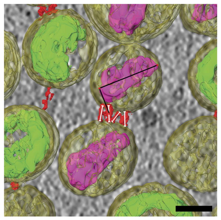
Figure 11.

Montage maps provide cellular context for cryo-ET data. (a) Montage of RSV A2-infected A549 cells taken at 10,000× using the energy filter for improved contrast. The cell membrane is regular and intact, with filamentous RSV protruding from it. Scale bar, 2 μm; inset scale bar, 500 nm. (b) Segmented cryo-ET data from inset in a indicating membrane (cyan), glycoproteins (yellow), RNP (red), and actin filaments (magenta). Data were collected at 8,000× on a DE-20 camera system. Binned by 2, pixel size is 14.94 Å. Scale bar, 500 nm.

Processing and combining of high-resolution CLEM overlay images ● TIMING 1 d

• 52|Perform z cropping, background adjustment, deconvolution, projection, and channel merging of cryo-fLM images (from Step 34) using the LASX software. For best results, separate the three channels and process them individually before merging them back together. The fluorescence signal of the specific probes is well maintained at cryo-fLM temperatures because there is minimal photobleaching^42,56,57, and the close working distance of the objective lens ensures that there is robust signal over background fluorescence. Merged fluorescence channels can be saved with and without the bright-field image.
• 53|Stitch together cryo-TEM montages (from Steps 46–47) to form maps using the eTomo software ‘Align Serial Sections/ Blend Montages’ function.
• 54|Scale and overlay both cryo-fLM and cryo-TEM maps in PhotoShop using layers. It is convenient to use the size and orientation of the holes in the carbon film to scale and rotate the images to one another (Figs. 9–11).

Processing of tilt series data ● TIMING 5–6 h per data set

• 55|Motion-correct the raw frames from the direct detector using the Python scripts (DE_combine_references.py and DE_process_frames.py) provided by Direct Electron (or other sources for different detectors). The total number of frames per image varies with the tilt angle because of the 1/cosine^1/5 exposure setting.
• 56|Recombine the corrected images using IMOD’s ‘newstack’ command. For bidirectional tilt series, we use the ‘reverse’ option. Create a corresponding rawtilt file containing all angles for the tilt series.
• 57|Launch 3dmod’s eTomo module, import the tilt series, and select ‘Tilt angles in existing rawtlt file’.
• 58|Perform coarse alignment, fiducial-based fine alignment, and tomogram positioning using the eTomo user interface.
• 59|Correct the CTF, create the full aligned stack, and then proceed with r-weighted back-projection^53,58. It is advisable to do binned and full versions of tomograms within the eTomo module by going back to the ‘Create Full Aligned Stack’ module in eTomo to create consistently scaled maps. Be sure to change the output .rec filename so that it is not overwritten. Tomograms may be optionally filtered or denoised by nonlinear anisotropic diffusion, or other filters such as band-pass, bilateral, or median filters, before segmentation^{20,48,53,59,60}.

Segmentation of tomograms ● TIMING 1–3 d

• 60|Segmentation of densities in the tomogram is useful for illustrative purposes and to obtain quantitative measurements from surface data. Two options are currently available: the basic modeling tools in 3dmod, and the more detailed 3D segmentations in Amira.

(A) Performance of initial contour segmentation of proteins and cell and viral membranes in 3dmod

1. Filter the tomogram (nonlinear anisotropic diffusion), if needed.

2. Create contours of components that are then meshed into surfaces using imodmesh.

3. Take manual measurements with the drawing tools feature, saving the ‘info text’ dialog to file.

4. Run and plot statistical analyses such as neighbor density analysis (nda program) and distances between objects (mtk program).

(B) Performance of detailed segmentation of membranes and molecules of interest in Amira

1. Import the binned and/or filtered tomogram into Amira and filter to smooth pixel edges and display as orthoslices.

   ▲ CRITICAL STEP Make sure that Amira does not flip the data. To correct improper flipping, select ‘rotate around y-axis’ after the volume is initially imported into the program.

2. Segment tomographic data semiautomatically in Amira. Use of the masking option is helpful in selecting continuous membranes. Note that the use of a Wacom Cintiq monitor is very helpful for direct, on-screen drawing of contours.

3. Create surfaces using ‘SurfaceGen’ and ‘Smooth Surface’ under the project tab to create a smoothed 3D surface model, then select ‘Surface View’ for visualization.

4. After segmentation, label objects with the 3D annotation tool, which is useful for making measurements. For segmented data, measurements can be made using the 2D and 3D length and angle tools. 2D and 3D measurements can be made in the orthoslice view and surfaces can be measured in 3D. Similarly, angles can be measured in both 2D and 3D. Make sure to name each measurement in the ‘measurement properties’ window, and then export them to a spreadsheet for quantification (Figs. 10–12).

Figure 10.

Cryo-CLEM imaging of retroviral endocytosis and fusion. (a–c) Double-labeled HIV-1 particles pseudotyped with avian sarcoma and leukosis virus (ASLV) Env glycoprotein. (a) Cryo-CLEM of ASLV Env pseudotyped HIV-1 particles bound to CV-1/TVA950 cells. Central region is the overlay of the cryo-EM montage onto the cryo-fLM image. Red square indicates the tomography data in b and c. (b) Tomographic slice, with segmentation, of ASLV Env pseudotyped HIV-1 particles undergoing endocytosis. The viral membrane (light blue) and mature core (yellow) are rendered. Clathrin cages (purple) surround several viral particles. (c) Enlargement of one clathrin cage (purple) surrounding a viral particle (light blue). Scale bars, (b) 250 nm, (c) 100 nm.

Figure 12.

Quantitative segmentation data of HIV-1 particles with tetherin. Cells are transfected with pNLenv1-deltaU and pEGFP-tetherin. Measurements made along segmented tethers (red) connecting HIV-1 virions (yellow, transparent) to each other, as indicated by the thin white lines. Orientation axes of the mature HIV-1 core (purple) are identified as black lines. Scale bar, 50 nm.

Particle picking for subvolume averaging ● TIMING 1 d

• 61|
  Selection of particles using EMAN2 (ref. 48). Load the tomogram (Step 59) into EMAN2’s boxer graphical user interface with the following example command line:

     e2spt_boxer.py tomogram.rec --invert --inmemory --low-pass=80
  

  Set the box size relatively small (4–10 pixels) to begin with to avoid box overlaps when selecting closely spaced particles. Use the xyz views to make certain that the boxes are well centered on the densities. Save the coordinates as ‘box file’.

• 62|Using IMOD’s ‘point2mod’ command, convert the boxed particle coordinates to a model file for use in alignment and averaging in PEET (Step 64).
• 63|Editing of the model file. Open the tomogram (from Step 59) and model file (from Step 62) with IMOD and save the model object points as ‘Scattered’. The IMOD command ‘imodtrans’ can be used to scale the model files so that particles can be picked in a binned tomogram and a corresponding model file can be made for the unbinned tomogram.

Subvolume alignment, averaging, and classification ● TIMING 1–6 months

• 64|There are several image processing packages that incorporate subvolume analysis, and here we highlight two that are commonly used in our group. Use option A to align and classify subvolumes using PEET and option b to do so using EMAN2.

(A) Alignment and classifying of subvolumes using PEET

1. Scale the PEET^49,50 motive list (.csv files) generated after initial alignments (in Excel) to match unbinned tomographic data. Use this file as input (under the PEET ‘Setup’ tab ‘Initial Motive List’) for running fine alignment. When running PEET, we typically select the option ‘save individual aligned particles’ (under the PEET ‘Run’ tab ‘Optional / Advance Features’). The individual aligned particles can be inspected in IMOD and screened manually to ensure that no misaligned particles are used to generate the final subvolume average. A final subvolume average of the manually screened aligned particles can be generated using the PEET command ‘averageAll’ or the IMOD command ‘clip’.

(B) Alignment and classification using EMAN2

1. With EMAN2’s ‘e2spt_classaverage.py’ script⁴⁷, use binned tomograms (binned by a factor of 2 or 4) to generate an initial subvolume average and to explore different alignment parameters, including box size, angular search range and search distance, and masking options, and selection of an appropriate starting reference.

? TROUBLESHOOTING

Troubleshooting advice can be found in Table 1.

TABLE 1.

Troubleshooting table.

Step	Problem	Possible reason	Solution
6	Grids float on the medium	Surface of grids is hydrophobic because of insufficient glow discharging Air bubbles are attached to the grid	Adjust the settings on the plasma cleaner (Step 5) Introduce grids into solutions slowly and vertically to avoid formation of bubbles (Step 6)
15, 31, 38	Carbon film is torn	Rough handling of the grids Forceps have been damaged Grids were allowed to dry out Carbon film was damaged during blotting	Handle grids gently Avoid using forceps with bent tips Do not aspirate grids to dryness (Steps 8 and 12; Box 1) Reduce compressed nitrogen gas PSI on Gatan CryoPlunge3 unit (Step 16)
	Too many cells on the grid	Seeding density is high Cells are over confluent	Use a lower initial seeding density (Step 13; Supplementary Table 1) Grow the cells for a shorter time (Step 14; Supplementary Table 1)
	Not enough cells on the grid	Low initial seeding density Cells are not adhering to the grid	Seed at a higher density (Step 13; Supplementary Table 1) Include growth factors or coat carbon with extracellular matrix proteins (Step 7; Box 1)
	Cells are too rounded	Low initial seeding density No extracellular matrix solutions applied to the grids Virus infection is too high	Seed at a higher density (Step 13; Supplementary Table 1) Coat carbon with extracellular matrix proteins (Step 7; Box 1) Lower MOI of virus (Step 15; Supplementary Table 2)
31, 38	Ice is too thick	Blotting conditions are inadequate Cells are too confluent	Use a longer blot time (Step 25) Remember to rotate blotters (Step 26) Reduce the seeding density (Step 14; Supplementary Table 1)
38	Ice is too thick on one half of the grid	Grid is not centered and held evenly in plunge device forceps	Make sure that tips of forceps do not extend past the rim of the grid (Step 21)
38, 48	Ice on the grid has a freckled appearance	Warming past the vitrification point (i.e., above –150 °C) has occurred	Check the temperature of the cryo-fLM stage (Step 28) and expedite grid transfers (Steps 27, 29, 35, and 37)
	Lots of cell debris in the ice	Cytotoxicity from virus infection or transfection Cells were damaged during blotting	Cryo-plunge at an earlier time point (Step 15; Supplementary Table 1) Add an extra or longer DPBS wash to remove debris (Step 22) Adjust the blot settings (Step 25)
	Cell membranes appear ruptured or blebby	Blotting conditions are too severe Grid became too dry before blotting Cells were exposed to low temperatures	Lessen the blot force (Step 25) Reduce exposure to air and evaporation (Steps 21–26) Reduce time spent out of the incubator Do not place culture dishes on a cold benchtop and avoid holding the grid near liquid nitrogen while loading the plunge rod (Step 24)
	Large amounts of solid ice particles on grid surface	Ice contamination from atmosphere	Do grid transfers in a humidity-controlled room (relative humidity <30%) Use Plexiglas shields or wear a facemask when transferring (Steps 27, 29, 35, and 37)
48	Gold fiducials aggregated in the ice	Initial solution of gold fiducials has precipitated	Vortex gold fiducial solution before use (Step 20)

● TIMING

• Steps 1–7, preparation of EM grids: ~1–2 d

• Steps 8–14, culture of cells on EM grids: 1–2 d

• Step 15, introduction of virus to cells: 30 min to 3 d

• Steps 16–27, vitrification of grids by plunge-freezing: 1 h

• Steps 28–36, cryo-fLM imaging: 30–45 min

• Steps 37–40, creation of low-magnification cryo-TEM maps: 20–30 min

• Steps 41–45, correlation of the TEM map with the CLEM map: 30 min

• Steps 46 and 47, intermediate-magnification montaging: 30–60 min

• Steps 48–51, tilt series acquisition: 6–18 h

• Steps 52–54, processing and combining of high-resolution CLEM overlay images: 1 d

• Steps 55–59, processing of tilt series data: 5–6 h per data set

• Step 60, segmentation of tomograms: 1–3 d

• Steps 61–63, particle picking for subvolume averaging: 1 d

• Step 64, subvolume alignment, averaging, and classification: 1–6 months

  Box 1, coating of grids with extracellular matrix components: 8–24 h

ANTICIPATED RESULTS

This protocol describes how to perform cryo-CLEM on intact, virus-infected or transfected mammalian cells. The success and quality of the acquired data depend heavily on the handling of the TEM grids during grid preparation, especially during transfers from the plunge-freezing apparatus to grid boxes and the microscopes. Figure 13 provides examples of suboptimal grids for cryo-CLEM imaging. Examples of ice contamination from the atmosphere and ice morphological changes due to warming are shown, as well as how grids that are bent or otherwise uneven do not produce maps that correlate well in either microscope.

Figure 13.

Examples of poor-quality grids for cryo-CLEM imaging. (a) A cryo-fLM map of a slightly bent grid produces focus gradients within each stitched image, preventing accurate localization of regions of interest. (b) A low-magnification cryo-EM grid map of a 3-mm grid that has been bent before cryo-EM imaging. Aside from the obvious missing carbon in most grid squares, there are large variations in z height. (c) Image showing ice over 2-μm holes in the Quantifoil carbon film. W indicates ice that has warmed above the transition temperature (~−150 °C) to create crystalline artifacts. x indicates ice contamination from the atmosphere that has landed on the grid. Both can be attributed to transfer steps.

References

- 1.Morgan C, Godman GC, Breitenfeld PM, Rose HM. A correlative study by electron and light microscopy of the development of type 5 adenovirus. I. Electron microscopy. J Exp Med. 1960;112:373–382. doi: 10.1084/jem.112.2.373. [DOI] [PMC free article] [PubMed] [Google Scholar]
- 2.Godman GC, Morgan C, Breitenfeld PM, Rose HM. A correlative study by electron and light microscopy of the development of type 5 adenovirus. II. Light microscopy. J Exp Med. 1960;112:383–402. doi: 10.1084/jem.112.2.383. [DOI] [PMC free article] [PubMed] [Google Scholar]
- 3.Dubochet J, et al. Cryo-electron microscopy of vitrified specimens. Q Rev Biophys. 1988;21:129–228. doi: 10.1017/s0033583500004297. [DOI] [PubMed] [Google Scholar]
- 4.Mancini EJ, de Haas F, Fuller SD. High-resolution icosahedral reconstruction: fulfilling the promise of cryo-electron microscopy. Structure. 1997;5:741–750. doi: 10.1016/s0969-2126(97)00229-3. [DOI] [PubMed] [Google Scholar]
- 5.Steven AC, Aebi U. The next ice age: cryo-electron tomography of intact cells. Trends Cell Biol. 2003;13:107–110. doi: 10.1016/s0962-8924(03)00023-0. [DOI] [PubMed] [Google Scholar]
- 6.Risco C, Carrascosa JL. Visualization of viral assembly in the infected cell. Histol Histopathol. 1999;14:905–926. doi: 10.14670/HH-14.905. [DOI] [PubMed] [Google Scholar]
- 7.Schroder RR. Advances in electron microscopy: a qualitative view of instrumentation development for macromolecular imaging and tomography. Arch Biochem Biophys. 2015;581:25–38. doi: 10.1016/j.abb.2015.05.010. [DOI] [PubMed] [Google Scholar]
- 8.McDonald KL. A review of high-pressure freezing preparation techniques for correlative light and electron microscopy of the same cells and tissues. J Microsc. 2009;235:273–281. doi: 10.1111/j.1365-2818.2009.03218.x. [DOI] [PubMed] [Google Scholar]
- 9.Carroni M, Saibil HR. Cryo electron microscopy to determine the structure of macromolecular complexes. Methods. 2016;95:78–85. doi: 10.1016/j.ymeth.2015.11.023. [DOI] [PMC free article] [PubMed] [Google Scholar]
- 10.Giepmans BN, Adams SR, Ellisman MH, Tsien RY. The fluorescent toolbox for assessing protein location and function. Science. 2006;312:217–224. doi: 10.1126/science.1124618. [DOI] [PubMed] [Google Scholar]
- 11.Desai TM, et al. Fluorescent protein-tagged Vpr dissociates from HIV-1 core after viral fusion and rapidly enters the cell nucleus. Retrovirology. 2015;12:88. doi: 10.1186/s12977-015-0215-z. [DOI] [PMC free article] [PubMed] [Google Scholar]
- 12.Padilla-Parra S, et al. Fusion of mature HIV-1 particles leads to complete release of a gag-GFP-based content marker and raises the intraviral pH. PLoS One. 2013;8:e71002. doi: 10.1371/journal.pone.0071002. [DOI] [PMC free article] [PubMed] [Google Scholar]
- 13.Briegel A, et al. Correlated light and electron cryo-microscopy. Methods Enzymol. 2010;481:317–341. doi: 10.1016/S0076-6879(10)81013-4. [DOI] [PubMed] [Google Scholar]
- 14.Strauss JD, et al. Three-dimensional structural characterization of HIV-1 tethered to human cells. J Virol. 2015;90:1507–1521. doi: 10.1128/JVI.01880-15. [DOI] [PMC free article] [PubMed] [Google Scholar]
- 15.Yi H, et al. Native immunogold labeling of cell surface proteins and viral glycoproteins for cryo-electron microscopy and cryo-electron tomography applications. J Histochem Cytochem. 2015;63:780–792. doi: 10.1369/0022155415593323. [DOI] [PMC free article] [PubMed] [Google Scholar]
- 16.Mastronarde DN. Automated electron microscope tomography using robust prediction of specimen movements. J Struct Biol. 2005;152:36–51. doi: 10.1016/j.jsb.2005.07.007. [DOI] [PubMed] [Google Scholar]
- 17.Bharat TA, Russo CJ, Lowe J, Passmore LA, Scheres SH. Advances in single-particle electron cryomicroscopy structure determination applied to sub-tomogram averaging. Structure. 2015;23:1743–1753. doi: 10.1016/j.str.2015.06.026. [DOI] [PMC free article] [PubMed] [Google Scholar]
- 18.Hrabe T. Localize.pytom: a modern webserver for cryo-electron tomography. Nucleic Acids Res. 2015;43:W231–236. doi: 10.1093/nar/gkv400. [DOI] [PMC free article] [PubMed] [Google Scholar]
- 19.Huiskonen JT, et al. Averaging of viral envelope glycoprotein spikes from electron cryotomography reconstructions using Jsubtomo. J Vis Exp. 2014:e51714. doi: 10.3791/51714. [DOI] [PMC free article] [PubMed] [Google Scholar]
- 20.Heymann JB, Cardone G, Winkler DC, Steven AC. Computational resources for cryo-electron tomography in Bsoft. J Struct Biol. 2008;161:232–242. doi: 10.1016/j.jsb.2007.08.002. [DOI] [PMC free article] [PubMed] [Google Scholar]
- 21.Castano-Diez D, Kudryashev M, Arheit M, Stahlberg H. Dynamo: a flexible, user-friendly development tool for subtomogram averaging of cryo-EM data in high-performance computing environments. J Struct Biol. 2012;178:139–151. doi: 10.1016/j.jsb.2011.12.017. [DOI] [PubMed] [Google Scholar]
- 22.Koning RI, et al. Correlative cryo-fluorescence light microscopy and cryo-electron tomography of Streptomyces. Methods Cell Biol. 2014;124:217–239. doi: 10.1016/B978-0-12-801075-4.00010-0. [DOI] [PubMed] [Google Scholar]
- 23.van Driel LF, Valentijn JA, Valentijn KM, Koning RI, Koster AJ. Tools for correlative cryo-fluorescence microscopy and cryo-electron tomography applied to whole mitochondria in human endothelial cells. Eur J Cell Biol. 2009;88:669–684. doi: 10.1016/j.ejcb.2009.07.002. [DOI] [PubMed] [Google Scholar]
- 24.Jun S, et al. Direct visualization of HIV-1 with correlative live-cell microscopy and cryo-electron tomography. Structure. 2011;19:1573–1581. doi: 10.1016/j.str.2011.09.006. [DOI] [PMC free article] [PubMed] [Google Scholar]
- 25.Ibiricu I, et al. Cryo electron tomography of herpes simplex virus during axonal transport and secondary envelopment in primary neurons. PLoS Pathog. 2011;7:e1002406. doi: 10.1371/journal.ppat.1002406. [DOI] [PMC free article] [PubMed] [Google Scholar]
- 26.Schorb M, Briggs JA. Correlated cryo-fluorescence and cryo-electron microscopy with high spatial precision and improved sensitivity. Ultramicroscopy. 2014;143:24–32. doi: 10.1016/j.ultramic.2013.10.015. [DOI] [PMC free article] [PubMed] [Google Scholar]
- 27.Briegel A, et al. Location and architecture of the Caulobacter crescentus chemoreceptor array. Mol Microbiol. 2008;69:30–41. doi: 10.1111/j.1365-2958.2008.06219.x. [DOI] [PMC free article] [PubMed] [Google Scholar]
- 28.Swulius MT, et al. Long helical filaments are not seen encircling cells in electron cryotomograms of rod-shaped bacteria. Biochem Biophys Res Commun. 2011;407:650–655. doi: 10.1016/j.bbrc.2011.03.062. [DOI] [PMC free article] [PubMed] [Google Scholar]
- 29.Chang YW, et al. Correlated cryogenic photoactivated localization microscopy and cryo-electron tomography. Nat Methods. 2014;11:737–739. doi: 10.1038/nmeth.2961. [DOI] [PMC free article] [PubMed] [Google Scholar]
- 30.Wang Q, Mercogliano CP, Lowe J. A ferritin-based label for cellular electron cryotomography. Structure. 2011;19:147–154. doi: 10.1016/j.str.2010.12.002. [DOI] [PubMed] [Google Scholar]
- 31.Gold VA, et al. Visualizing active membrane protein complexes by electron cryotomography. Nat Commun. 2014;5:4129. doi: 10.1038/ncomms5129. [DOI] [PMC free article] [PubMed] [Google Scholar]
- 32.Mercogliano CP, DeRosier DJ. Concatenated metallothionein as a clonable gold label for electron microscopy. J Struct Biol. 2007;160:70–82. doi: 10.1016/j.jsb.2007.06.010. [DOI] [PMC free article] [PubMed] [Google Scholar]
- 33.Al-Amoudi A, et al. Cryo-electron microscopy of vitreous sections. EMBO J. 2004;23:3583–3588. doi: 10.1038/sj.emboj.7600366. [DOI] [PMC free article] [PubMed] [Google Scholar]
- 34.Gruska M, Medalia O, Baumeister W, Leis A. Electron tomography of vitreous sections from cultured mammalian cells. J Struct Biol. 2008;161:384–392. doi: 10.1016/j.jsb.2007.10.008. [DOI] [PubMed] [Google Scholar]
- 35.Engel BD, et al. Native architecture of the Chlamydomonas chloroplast revealed by in situ cryo-electron tomography. Elife. 2015;4:e04889. doi: 10.7554/eLife.04889. [DOI] [PMC free article] [PubMed] [Google Scholar]
- 36.Marko M, Hsieh C, Schalek R, Frank J, Mannella C. Focused-ion-beam thinning of frozen-hydrated biological specimens for cryo-electron microscopy. Nat Methods. 2007;4:215–217. doi: 10.1038/nmeth1014. [DOI] [PubMed] [Google Scholar]
- 37.Wolf SG, Houben L, Elbaum M. Cryo-scanning transmission electron tomography of vitrified cells. Nat Methods. 2014;11:423–428. doi: 10.1038/nmeth.2842. [DOI] [PubMed] [Google Scholar]
- 38.Bykov YS, Cortese M, Briggs JA, Bartenschlager R. Correlative light and electron microscopy methods for the study of virus-cell interactions. FEBS Lett. 2016;590:1877–1895. doi: 10.1002/1873-3468.12153. [DOI] [PubMed] [Google Scholar]
- 39.Schellenberger P, et al. High-precision correlative fluorescence and electron cryo microscopy using two independent alignment markers. Ultramicroscopy. 2014;143:41–51. doi: 10.1016/j.ultramic.2013.10.011. [DOI] [PMC free article] [PubMed] [Google Scholar]
- 40.Liu B, et al. Three-dimensional super-resolution protein localization correlated with vitrified cellular context. Sci Rep. 2015;5:13017. doi: 10.1038/srep13017. [DOI] [PMC free article] [PubMed] [Google Scholar]
- 41.Wolff G, Hagen C, Grunewald K, Kaufmann R. Towards correlative super-resolution fluorescence and electron cryo-microscopy. Biol Cell. 2016;108:245–258. doi: 10.1111/boc.201600008. [DOI] [PMC free article] [PubMed] [Google Scholar]
- 42.Schwartz CL, Sarbash VI, Ataullakhanov FI, McIntosh JR, Nicastro D. Cryo-fluorescence microscopy facilitates correlations between light and cryo-electron microscopy and reduces the rate of photobleaching. J Microsc. 2007;227:98–109. doi: 10.1111/j.1365-2818.2007.01794.x. [DOI] [PubMed] [Google Scholar]
- 43.Sartori A, et al. Correlative microscopy: bridging the gap between fluorescence light microscopy and cryo-electron tomography. J Struct Biol. 2007;160:135–145. doi: 10.1016/j.jsb.2007.07.011. [DOI] [PubMed] [Google Scholar]
- 44.Rigort A, et al. Micromachining tools and correlative approaches for cellular cryo-electron tomography. J Struct Biol. 2010;172:169–179. doi: 10.1016/j.jsb.2010.02.011. [DOI] [PubMed] [Google Scholar]
- 45.Faas FG, et al. Localization of fluorescently labeled structures in frozen-hydrated samples using integrated light electron microscopy. J Struct Biol. 2013;181:283–290. doi: 10.1016/j.jsb.2012.12.004. [DOI] [PubMed] [Google Scholar]
- 46.Schorb M, et al. New hardware and workflows for semi-automated correlative cryo-fluorescence and cryo-electron microscopy/tomography. J Struct Biol. 2016 doi: 10.1016/j.jsb.2016.06.020. https://dx.doi.org/10.1016/j.jsb.2016.06.020. [DOI] [PMC free article] [PubMed]
- 47.Galaz-Montoya JG, Flanagan J, Schmid MF, Ludtke SJ. Single particle tomography in EMAN2. J Struct Biol. 2015;190:279–290. doi: 10.1016/j.jsb.2015.04.016. [DOI] [PMC free article] [PubMed] [Google Scholar]
- 48.Tang G, et al. EMAN2: an extensible image processing suite for electron microscopy. J Struct Biol. 2007;157:38–46. doi: 10.1016/j.jsb.2006.05.009. [DOI] [PubMed] [Google Scholar]
- 49.Nicastro D, et al. The molecular architecture of axonemes revealed by cryoelectron tomography. Science. 2006;313:944–948. doi: 10.1126/science.1128618. [DOI] [PubMed] [Google Scholar]
- 50.Heumann JM, Hoenger A, Mastronarde DN. Clustering and variance maps for cryo-electron tomography using wedge-masked differences. J Struct Biol. 2011;175:288–299. doi: 10.1016/j.jsb.2011.05.011. [DOI] [PMC free article] [PubMed] [Google Scholar]
- 51.Winkler H. 3D reconstruction and processing of volumetric data in cryo-electron tomography. J Struct Biol. 2007;157:126–137. doi: 10.1016/j.jsb.2006.07.014. [DOI] [PubMed] [Google Scholar]
- 52.Huiskonen JT, et al. Electron cryotomography of Tula hantavirus suggests a unique assembly paradigm for enveloped viruses. J Virol. 2010;84:4889–4897. doi: 10.1128/JVI.00057-10. [DOI] [PMC free article] [PubMed] [Google Scholar]
- 53.Kremer JR, Mastronarde DN, McIntosh JR. Computer visualization of three-dimensional image data using IMOD. J Struct Biol. 1996;116:71–76. doi: 10.1006/jsbi.1996.0013. [DOI] [PubMed] [Google Scholar]
- 54.Rohou A, Grigorieff N. CTFFIND4: fast and accurate defocus estimation from electron micrographs. J Struct Biol. 2015;192:216–221. doi: 10.1016/j.jsb.2015.08.008. [DOI] [PMC free article] [PubMed] [Google Scholar]
- 55.Hagen WJ, Wan W, Briggs JA. Implementation of a cryo-electron tomography tilt-scheme optimized for high resolution subtomogram averaging. J Struct Biol. 2016 doi: 10.1016/j.jsb.2016.06.007. [DOI] [PMC free article] [PubMed] [Google Scholar]
- 56.Moerner WE, Orrit M. Illuminating single molecules in condensed matter. Science. 1999;283:1670–1676. doi: 10.1126/science.283.5408.1670. [DOI] [PubMed] [Google Scholar]
- 57.Kaufmann R, Hagen C, Grunewald K. Fluorescence cryo-microscopy: current challenges and prospects. Curr Opin Chem Biol. 2014;20:86–91. doi: 10.1016/j.cbpa.2014.05.007. [DOI] [PMC free article] [PubMed] [Google Scholar]
- 58.Xiong Q, Morphew MK, Schwartz CL, Hoenger AH, Mastronarde DN. CTF determination and correction for low dose tomographic tilt series. J Struct Biol. 2009;168:378–387. doi: 10.1016/j.jsb.2009.08.016. [DOI] [PMC free article] [PubMed] [Google Scholar]
- 59.Heymann JB, Belnap DM. Bsoft: image processing and molecular modeling for electron microscopy. J Struct Biol. 2007;157:3–18. doi: 10.1016/j.jsb.2006.06.006. [DOI] [PubMed] [Google Scholar]
- 60.Heymann JB. Bsoft: image and molecular processing in electron microscopy. J Struct Biol. 2001;133:156–169. doi: 10.1006/jsbi.2001.4339. [DOI] [PubMed] [Google Scholar]
Associated Data
This section collects any data citations, data availability statements, or supplementary materials included in this article.