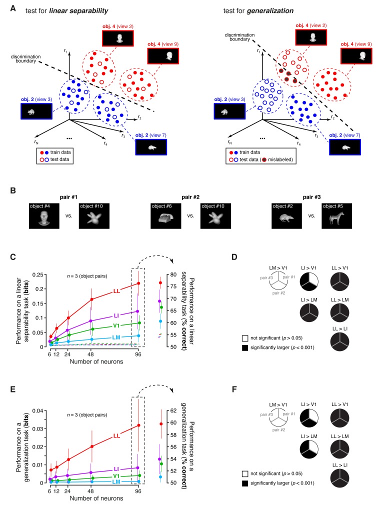
Figure 8. Linear separability and generalization of object representations, tested at the level of neuronal populations.

(A) Illustration of the population decoding analyses used to test linear separability and generalization. The clouds of dots show the sets of response population vectors produced by different views of two objects. Left: for the test of linear separability, a binary linear decoder is trained with a fraction of the response vectors (filled dots) to all the views of both objects, and then tested with the left-out response vectors (empty dots), using the previously learned discrimination boundary (dashed line). The cartoon depicts the ideal case of two object representations that are perfectly separable. Right: for the test of generalization, a binary linear decoder is trained with all the response vectors (filled dots) produced by a single view per object, and then tested for its ability to correctly discriminate the response vectors (empty dots) produced by the other views, using the previously learned discrimination boundary (dashed line). As illustrated here, perfect linearly separability does not guarantee perfect generalization to untrained object views (see the black-filled, mislabeled response vectors in the right panel). (B) The three pairs of visual objects that were selected for the population decoding analyses shown in C-F, based on the fact that their luminance ratio fulfilled the constraint of being larger than ${\displaystyle T{h}_{LumRatio}=0.8}$ for at least 96 neurons in each area. (C) Classification performance of the binary linear decoders in the test for linear separability, as a function of the number of neurons N used to build the population vector space. Performances were computed for the three pairs of objects shown in (B). Each dot shows the mean of the performances obtained for the three pairs (± SE). The performances are reported as the mutual information between the actual and the predicted object labels (left). In addition, for N = 96, they are also shown in terms of classification accuracy (right). The dashed lines (left) and the horizontal marks (right) show the linear separability of arbitrary groups of views of two objects (same three pairs used in the main analysis; see Results). (D) The statistical significance of each pairwise area comparison, in terms of linear separability, is reported for each individual object pair (1-tailed U-test, Holm-Bonferroni corrected). In the pie charts, a black slice indicates that the test was significant (p<0.001) for the corresponding pairs of objects and areas (e.g., LL > LI). (E) Classification performance of the binary linear decoders in the test for generalization across transformations. Same description as in (C). (F) Statistical significance of each pairwise area comparison, in terms of generalization across transformations. Same description as in (D). The same analyses, performed over a larger set of object pairs, after setting $T{h}_{LumRatio}=0.6$, are shown in Figure 8—figure supplement 1. The dependence of linear separability and generalization from $T{h}_{LumRatio}$ is shown in Figure 8—figure supplement 2. The statistical comparison between the performances achieved by a population of 48 LL neurons and V1, LM and LI populations of 96 neurons is reported in Figure 8—figure supplement 3.

DOI: http://dx.doi.org/10.7554/eLife.22794.023

Figure 8—figure supplement 1. Linear separability and generalization of object representations, tested at the level of neuronal populations, using a larger set of object pairs.

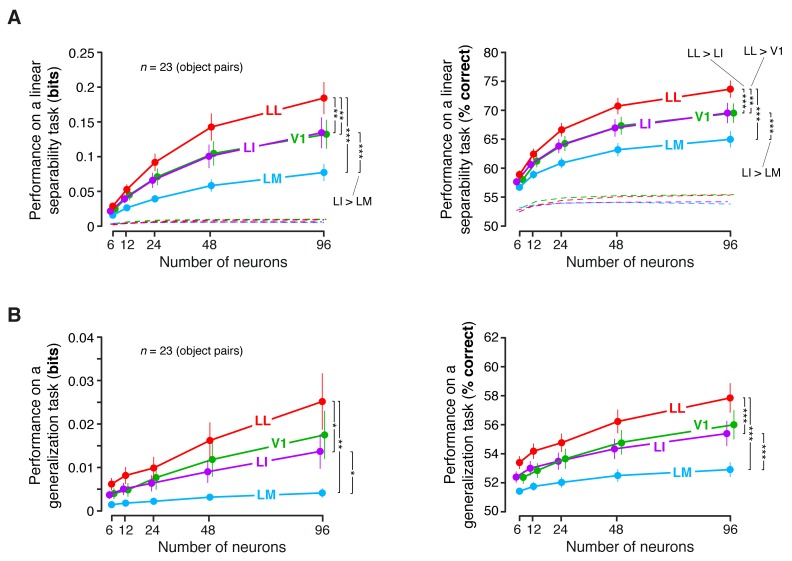
(A) Classification performance of binary linear decoders in the test for linear separability (see Figure 8A, left), as a function of the size of the neuronal subpopulations used to build the population vector space. This plot is equivalent to the one shown in Figure 8C, with the difference that, here, the objects that the decoders had to discriminate were allowed to differ more in terms of luminosity (this was achieved by setting $T{h}_{LumRatio}=0.6$). As a result, much more object pairs (23) could be tested, compared to the analysis shown in Figure 8C. Each dot shows the mean of the 23 performances obtained for these object pairs and the error bar shows its SE. The larger number of object pairs allowed applying a 1-tailed, paired t-test (with Holm-Bonferroni correction) to assess whether the differences among the average performances in the four areas were statistically significant (*p<0.05, **p<0.01, ***p<0.001). The performances are reported both as mutual information between actual and predicted object labels (left) and as classification accuracy (i.e., as the percentage of correctly labeled response vectors; right). (B) Classification performance of binary linear decoders in the test for generalization across transformations (see Figure 8A, right). Same description as in (A).

DOI: http://dx.doi.org/10.7554/eLife.22794.024

Figure 8—figure supplement 2. Dependence of linear separability and generalization, measured at the neuronal population level, from the luminance difference of the objects to discriminate.

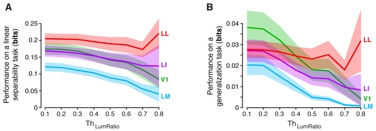
(A) Classification performance of binary linear decoders in the test for linear separability (see Figure 8A, left) as a function of the similarity between the RF luminance of the objects to discriminate, as defined by $T{h}_{LumRatio}$ (see Results). The curves, which were produced using populations of 96 neurons, report the median performance in each visual area (± SE) over all the object pairs obtained for a given value of $T{h}_{LumRatio}$. Note that, for $T{h}_{LumRatio}=0.8$ and $T{h}_{LumRatio}=0.6$, the performances are equivalent to those already shown in the left panels Figure 8C and Figure 8—figure supplement 1A (rightmost points). Also note that, for $T{h}_{LumRatio}=0.1$, all the available object pairs contributed to the analysis. As such, the corresponding performances are those yielded by the four visual areas when no restriction was applied to the luminosity of the objects to discriminate. (B) Same analysis as in (A), but for the test of generalization across transformations (see Figure 8A, right).

DOI: http://dx.doi.org/10.7554/eLife.22794.025

Figure 8—figure supplement 3. Statistical comparison between the performance achieved by a population of 48 LL neurons and the performances yielded by populations of 96 neurons in V1, LM and LI.

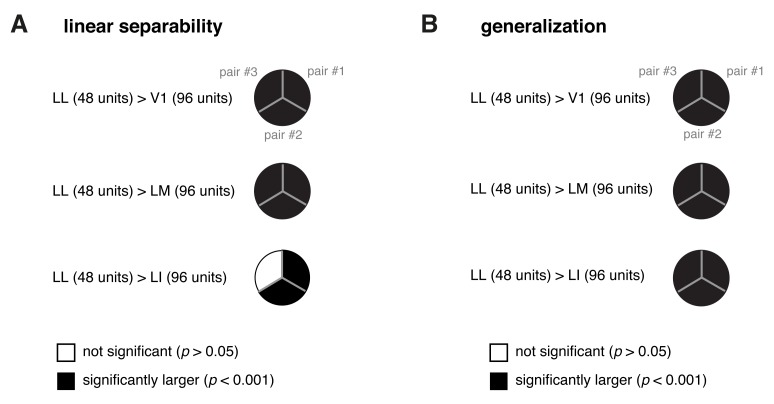
(A) For each of the three object pairs tested in Figure 8 (shown in Figure 8B), we checked whether a population of 48 LL neurons yielded a significantly larger performance than V1, LM and LI populations of twice the number of neurons (i.e., 96 units) in the linear discriminability task (see Figure 8A, left). The resulting pie chart shown here should be compared to the rightmost column of the pie chart in Figure 8D, with a black slice indicating that the comparison was significant (p<0.001; 1-tailed U-test, Holm-Bonferroni corrected) for the corresponding pairs of objects and areas – e.g., LL (48 units) > LI (96 units). (B) Same analysis as in (A), but for the test of generalization across transformations (see Figure 8A, right). The pie chart shown here should be compared to the rightmost column of the pie chart in Figure 8F.

DOI: http://dx.doi.org/10.7554/eLife.22794.026