Probabilistic models of species discovery and biodiversity comparisons

Significance

Estimates of species numbers are central to many analyses in fields ranging from conservation biology to macroecology and macroevolution. However, new species continue to be discovered and described at an uneven rate among regions and taxonomic groups, raising questions about the robustness of currently observed biodiversity patterns. We present a statistical approach to the rate of species description that incorporates uncertainty in species numbers across space and among clades. This approach identifies regions or clades where taxonomic knowledge is most complete, and provides estimates of stability in large-scale patterns given continued species discoveries through probabilistic forecasts of diversity levels.

Abstract

Inferring large-scale processes that drive biodiversity hinges on understanding the phylogenetic and spatial pattern of species richness. However, clades and geographic regions are accumulating newly described species at an uneven rate, potentially affecting the stability of currently observed diversity patterns. Here, we present a probabilistic model of species discovery to assess the uncertainty in diversity levels among clades and regions. We use a Bayesian time series regression to estimate the long-term trend in the rate of species description for marine bivalves and find a distinct spatial bias in the accumulation of new species. Despite these biases, probabilistic estimates of future species richness show considerable stability in the currently observed rank order of regional diversity. However, absolute differences in richness are still likely to change, potentially modifying the correlation between species numbers and geographic, environmental, and biological factors thought to promote biodiversity. Applied to scallops and related clades, we find that accumulating knowledge of deep-sea species will likely shift the relative richness of these three families, emphasizing the need to consider the incomplete nature of bivalve taxonomy in quantitative studies of its diversity. Along with estimating expected changes to observed patterns of diversity, the model described in this paper pinpoints geographic areas and clades most urgently requiring additional systematic study—an important practice for building more complete and accurate models of biodiversity dynamics that can inform ecological and evolutionary theory and improve conservation practice.

The number of biological species on Earth is notoriously uncertain, but such estimates are critical for a broad range of issues, from the environmental and biological limits of diversity to the design of conservation strategies in dwindling habitats (1–6). Geographic and phylogenetic differences in the discovery and description of species can change the patterns of species richness that are used, for example, to pinpoint biodiversity hotspots (7). A frequent approach to either anticipating or evaluating these taxonomically driven shifts is to estimate the “true,” unknown species richness from a cumulative taxonomic description curve (8–10).

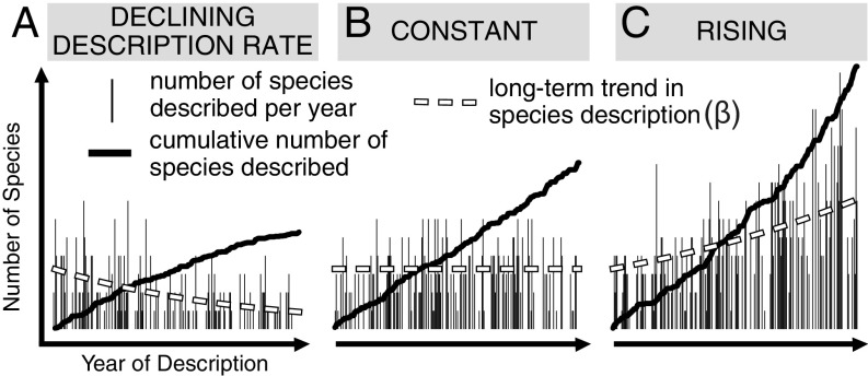
In theory, the cumulative count of newly described species should approach an asymptote as knowledge of the species pool nears the true value (Fig. 1A). However, many curves fail to “level off” or “saturate” because new species are being named at a steady or even accelerating rate (Fig. 1 B and C) (11, 12). These “unsaturated” curves lack a stable asymptote and therefore cannot provide robust estimates of the true species richness (12)—a result reflected in the many incongruent estimates of global diversity (13). Even with a robust estimate, a single value for the global number of species, or for high-level taxa such as Aves or Mammalia, is of limited utility in comparative diversity analyses across space, phylogeny, and time. Here, we develop a Bayesian model that can both accommodate nonasymptotic trends in species description to forecast species richness and operate at higher spatial and phylogenetic resolution. We use this model to assess the stability of observed differences in regional and among-clade diversity for a major animal group that has accrued newly described species at an unabated rate for the past 165 years: the marine bivalves.

Fig. 1.

Simulation of species description series under different long-term trends ($\beta$ in Modeling Taxonomic Description). (A) A declining description rate produces the “saturated” asymptotic cumulative description curve. Constant and rising trends in description produce cumulative description curves with (B) linear and (C) exponential shapes.

In our Bayesian time series model [available from Zenodo (doi.org/10.5281/zenodo.159033)], the number of species described in a given year is a function of the long- and short-term trends in description rate. We first model the trajectory of species accumulation using only the history of currently valid species description beginning with Linnaeus (14), the starting point of formal taxonomy. We then add a simple estimate of taxonomic effort (TE), another factor relevant to estimates of taxonomic knowledge (15–19). For both approaches, we find strong regional differences in the long-term trend of species description, suggesting a spatial bias in the saturation of taxonomic knowledge. We also identify potential instability in the relative richness of closely related clades but find that, overall, the major geographic and phylogenetic diversity patterns in our example are robust to the spatial and taxonomic heterogeneity of description rates. Thus, these probabilistic estimates can be useful measures of data stability in comparative analyses of diversity when focal regions or clades have not reached taxonomic saturation.

Modeling Taxonomic Description

Model Design.

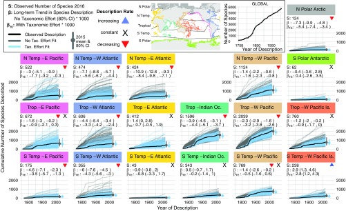
Our model most closely resembles that of refs. 4, 10, and 11, with three key differences. (i) We balance our prediction of species description events by modeling the short-term volatility and the long-term trend in the description rate (including consecutive years with no description). (ii) We shift our analytical focus from attempting to calculate a single, unknown true species richness (as in ref. 11) to estimating the aforementioned long-term trend in the number of species described per year ($\beta$, Fig. 1). This approach can be applied to any species description curve regardless of its asymptotic shape. For example, we can directly compare the degree of taxonomic saturation for two regions with dramatically different description trajectories—the North (N) Temperate East Atlantic and the Tropical West Pacific margin (Fig. 2). (iii) We simultaneously estimate model parameters for all groups (i.e., regions and clades) in a hierarchical Bayesian framework so that diversity estimates can be compared among groups (estimates are relative to each other and the overall “average” regional pattern) (20). Thus, parameter estimates for groups with low statistical power (low species counts and/or erratic description events) are drawn toward the average regional pattern, whereas parameter estimates from regions with high statistical power vary more freely. This approach makes group estimates appropriately conservative when statistical power is highly uneven. Altogether, these three model features improve the characterization of taxonomic description at regional scales and clade levels where description events can be irregular in time and number.

Fig. 2.

Description of marine bivalves species recognized at a water depth of <200 m across geographic regions (climate zones and coastlines marked in Inset map). Each regional panel plots the cumulative species description curve (dark black line) and 200 modeled description curves for TE and noTE fits (blue and gray lines respectively). Summary boxes report the total number of species recognized in the region today (S), the long-term trend in species described per year $\beta$ with its 80% credible interval, the long-term trend in species described per publication per year ${\beta }_{\text{TE}}$, and a colored symbol marking the sign of the long-term description trend (red down arrow, credible decline; blue up arrow, credible increase; and black X, no credible trend, i.e., constant). Model fits are plotted separately in Fig. S1. Is, islands; Oc, ocean.

Fig. S1.

Cumulative count of described species through time per geographic region. The range of the y axis is set by region-specific counts, to better visualize model fits within regions. Lines are the same as in Fig. 2, where gray lines are model fits without TE, blue lines are fits with TE, and black lines are the observed description series. Point ranges at the end of the description series show the predicted 2016 richness with 80% credible intervals. The range of model estimates for 2016 (median estimate and 80% CI to right of each time series) bracket the observed counts across all regions for models fit with and without TE, indicating that both models successfully predict the observed count of species today.

Incorporating TE.

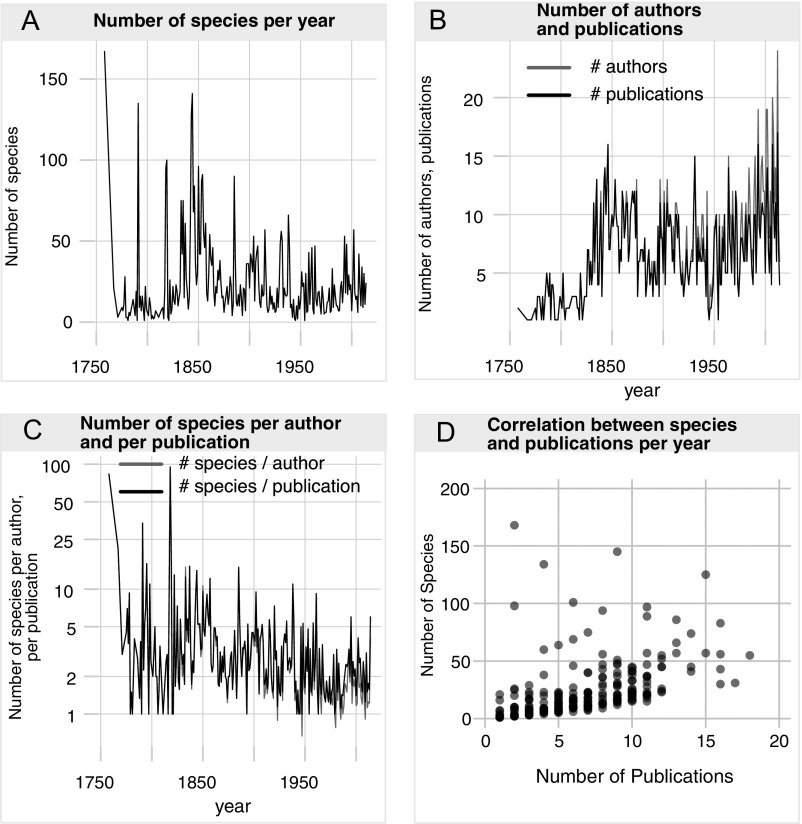
In theory, an approach toward true taxonomic knowledge should be reflected by a decline in species description rate and an increase in TE—a broad concept largely distilled into the time, energy, and funds required to discover and describe a new species. Trends in TE and species description are often studied in parallel (15–19), but are difficult to bring into the same model framework (12, 16). When modeled simultaneously, trends in TE and species description mutually inform estimates of taxonomic saturation. Here, we follow the logic of “catch per unit effort” (12) and model the number of publications as an exposure term in our Poisson regression, where the long-term trend becomes the number of species described per publication per year (Fig. S2). Thus, we might infer an approach toward taxonomic saturation from a decline in the number of species described per publication—lower catch per unit effort. This metric must be used cautiously because the steady attrition of professional taxonomists and the rise of nonprofessional publications (21, 22) drives a tendency for publications devoted to describing a single species. Thus, we cannot differentiate an increase in TE, i.e., an approach toward the true taxonomic knowledge, from a cultural shift to publishing in stand-alone journal articles rather than larger monographs.

Fig. S2.

Measure of TE through time. (A) The number of species described each year largely declines over time. (B) The number of publications and authors increases over time. (C) The number of species described per author and per publication declines over time. (D) The number of species described in a given year tends to be roughly proportional to the number of taxonomic publications in that year.

We adopt this publications-per-year metric because alternative measures of TE are difficult to compile and apply across a variety of biological groups and are subject to their own biases in taxonomic culture [e.g., the number of authors per species, the number of junior synonyms, the number of journal or book pages dedicated to a species, and the average time required to describe a new species (19)]. We emphasize that the simple metric used here is only a first step toward evaluating the role of TE in developing a more robust and complete probabilistic model of species discovery.

Results and Discussion

Our primary goal is to shift the use of species description histories away from estimating global richness toward comparing differences among regions and clades. To that end, we estimate the long-term species description rate, examine the utility of one estimate of TE, and forecast the stability of ranked regional and clade richness.

Comparing Model Performance.

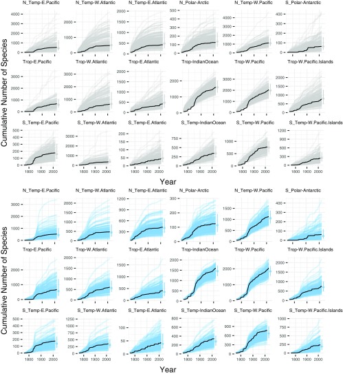
Posterior predictive simulations show that both model fits, with and without the addition of TE, accurately recover the observed species richness values in 2016, albeit by very different trajectories (compare median estimates and their credible intervals in Fig. 2). The model without TE (noTE) fails to follow the exponential, 1800–1860 spike in description, but does track the constant description from 1860 to today (e.g., Tropical West Pacific margin in Fig. 2). The TE model follows both the exponential spike in description and the transition to a more constant rate. Including the number of publications in the TE model smooths the expected description events through time by transforming the modeled value to a rate—the number of species described per publication per year. Thus, the short-term trends in description rate become more predictable because the year-to-year variance in the number of species per publication per year is considerably lower than the number of species described per year (Fig. S3). Therefore, the TE model has a tighter tracking of the description trajectory that leads to a more constrained estimate of present-day richness.

Fig. S3.

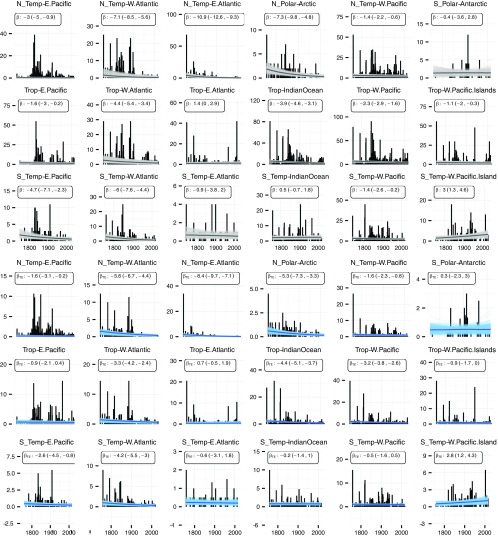
Fit of the long-term trend in species description to the observed count of descriptions per year. Top three rows show the model fit without TE (i.e., the number of species described per year), and the bottom three rows show the fit with TE (i.e., the number of species described per publication per year). Note that the black vertical segments are the numbers of species described in a year. Single dark gray and blue lines are the median long-term trend estimates ($\beta$), for the model fits with and without TE, respectively. The light gray and blue lines are 200 posterior predictive simulations of the long-term trends for the models without and with TE, respectively. Panels show the median estimated long-term trend and 80% credible interval same as in Fig. 2. The overall rank order of long-term trend coefficients is similar between models fit with and without TE. Temp, temperate; Trop, tropical.

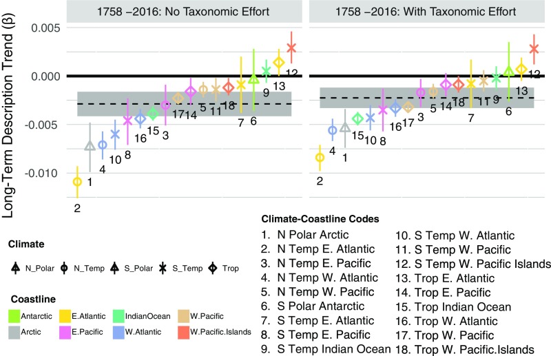
Long-term trends are not directly comparable between models because of the differences in their units ($\beta ={\text{N}}_{\text{species}}$ described per year; ${\beta }_{\text{TE}}={\text{N}}_{\text{species}}$ described per publication per year). However, the rank order of trend estimates remains consistent across both model fits (Figs. S4 and S5), likely reflecting a correlated decline in the number of publications and number of species described per year (Fig. S2).

Fig. S4.

Long-term trend coefficients for species description among regions. Symbols mark the median estimate, and bar represents the 80% credible interval. The horizontal dashed black lines mark the median estimated long-term trend of description rate among regions (80% credible interval in gray polygon). The overall rank order of long-term trend coefficients is similar between models fit with and without TE. Temp, temperate; Trop, tropical.

Fig. S5.

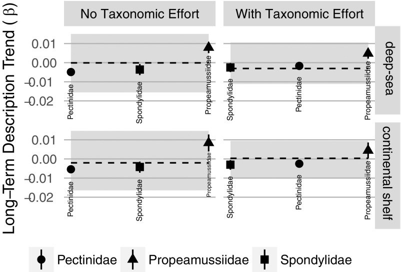
Long-term trend coefficients for species description among clades. Symbols mark the median estimate, and bar represents the 80% credible interval. The horizontal dashed black lines mark the median estimated long-term trend of description rate (80% credible interval in gray polygon). As with regions (Fig. S3), the overall rank order of long-term trend coefficients is similar between models fit with and without TE, for both the deep-sea and continental shelf datasets.

Geographic Variation in Species Description.

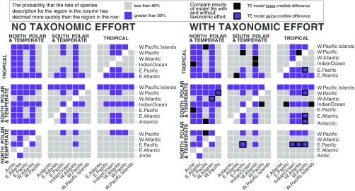
Globally, bivalve systematists have slowed in their description of new species over time. This overall decline is inevitable because of the shift near 1860 from a rising description rate to a remarkably constant description rate of 21 (20 to 22 ${\text{CI}}_{80\%}$) new species per year (Global, Fig. 2). Regionally, we find striking heterogeneity, where 12 of 18 climate–coastline regions show a decline in the number of species named per year (negative long-term trends $\beta$; red arrows in Fig. 2), five show constant description rates (black Xs), and only one shows a rising rate (blue arrow). In general, N Polar/Temperate coastlines have the strongest declines in description rate, followed by Tropical and then South (S) Polar/Temperate coastlines. Across climate zones, coastlines in the West Atlantic show some of the strongest declines in description rates, and those in the East Atlantic and West Pacific Islands show the weakest declines (Fig. S6).

Fig. S6.

Pairwise probabilities of differences in long-term description trends among climate–coastlines. For example, in the model without TE, there is at least an 80% probability that the long-term trend in description rate for the North Polar Arctic coastline (labeled column) has declined more rapidly than the trend for the North Temperate East Pacific (labeled row).

The variation in regional rates of species description highlights a distinct spatial bias in the history of bivalve systematics. As with many other groups, formal description of bivalve species began in 1758 (14) and was pursued with zest for another 100 years by several prolific European systematists (e.g., Gmelin, Lamarck, Reeve, and Deshayes). Consequently, the N Temperate East Atlantic exhibits the strongest decline in description rate, likely reflecting the most complete taxonomic knowledge of any region. However, proximity to the early European systematists does not impart a similar level of taxonomic saturation on Tropical and S Temperate East Atlantic coastlines. Our model identifies these regions as two of the least described (Fig. S4), even compared with coastlines in the Tropical Indian and West Pacific Oceans that are considered highly undersampled (23).

More than half of the climate–coastlines show a decline in the number of species described per publication per year, which implies a decline in the catch per unit effort under the assumption of constant taxonomic culture. Thus, these regions may be nearing taxonomic saturation, but this inference must be made cautiously, because, as noted above, decreases in scientific funding and political limitations on sampling might also drive the description declines. Regardless of the link between description rates and taxonomic completeness, the variation in description rates among geographic regions indicates spatial differences in taxonomic activity that must be accounted for in comparisons of their observed species richness.

Geographic Comparisons of Species Richness.

The long-term trends in description rates across geographic regions vary in sign, magnitude, and credibility, which, together, provide a relative sense of taxonomic activity. For example, the long-term trend in description rate is steeper in the Tropical West Pacific Islands than on the Tropical West Pacific margin, implying the West Pacific Islands are a comparatively undersaturated region (Fig. 2 and Fig. S3). However, estimating differences in diversity depends not only on the long-term trend in description but also on the baseline description rate (Fig. S3) and the current differences in observed diversity. Forecasts of species richness capture the effects of all of the factors above and become a useful tool for generating probabilistic estimates of species richness that help prevent overinterpretation in macroecological and macroevolutionary analyses (3, 24–26).

Forecasts of species richness after infinite time and effort could provide estimates of the true, unknown species richness. However, such estimates from our model accumulate a large forecasting error under the assumption that current trends in description rates will continue indefinitely (Fig. S7). Within the bivalve description series, poorest forecasting performance occurs during periods of relatively rapid change in description rate (1820–1860). Even during the long period of approximately constant global description (post-1860), longer forecasts create larger forecasting error, demonstrating that even small changes in description rate can compound into high predictive error. Thus, the credibility of a particular forecasting window depends on the likelihood that description rates remain constant, and that the size of the forecasting error is not comparable to the currently observed differences in diversity. Given these limitations, we conservatively interpret regional stability using a 20-y forecast, but we also compare those conservative estimates to a 50-y forecast with much greater inherent forecasting error.

Fig. S7.

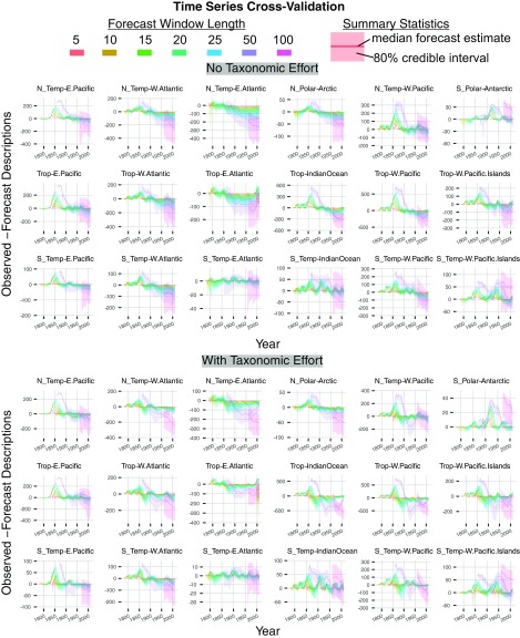
The forecasting error of the taxonomic description model. The y axis represents the forecasting error: the difference between the number of observed and forecast descriptions within the forecasting window. A value of zero means a perfect match between the observed and forecast values. Values above zero represent underprediction of species descriptions, and values below zero represent overprediction. For example, in the North Temperate East Pacific, there are ∼200 more species observed in 1855 than expected under the 50-y forecast. Poorest forecasting error occurs early in the taxonomic time series, during the exponential phase of species description. The forecasting error increases as the regional description series approach a more constant description rate. Forecasts tend to underpredict species richness in regions with rising long-term trends in description (see Fig. S4 and the South Temperate West Pacific Islands). Forecasts tend to overpredict in regions with declining trends in description (e.g., the N Temperate East Atlantic). Temp, temperate; Trop, tropical.

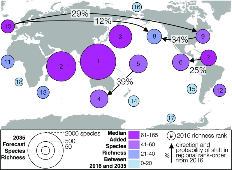
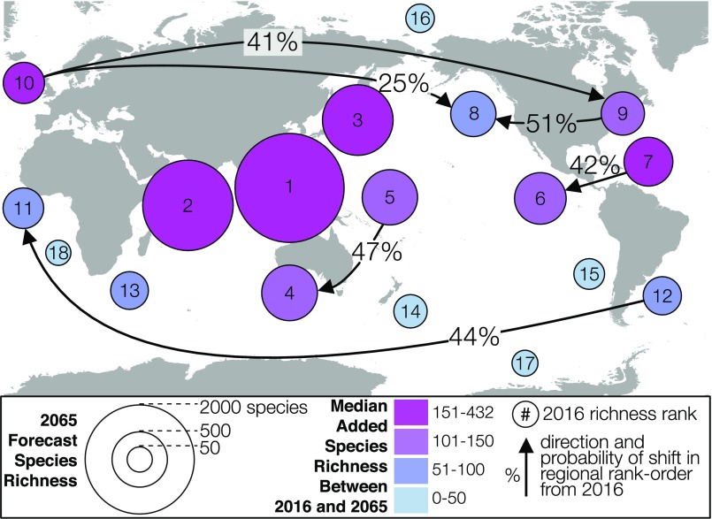
Despite the regional heterogeneity in description rate, we find an overall stability in the estimated rank order of regional diversity in 2035 and 2065 (Fig. 3, Fig. S8, and Table S1). Forecasts from both the TE and noTE models show that regions within the Indo-West Pacific are expected to gain the bulk of newly described species and will remain the richest. A mixture of Tropical and Temperate coastlines will continue to occupy the middle richness ranks, with Polar regions toward the lowest ranks. A few regions show nonzero but low probabilities of diversity rank shift across the 20- and 50-y forecasts (Fig. 3 and Fig. S8). These unlikely shifts are mostly confined within climate zones, implying that the global latitudinal diversity gradient will persist in light of continued species discovery.

Fig. 3.

The 20-y forecast of species richness (noTE model year 2035); forecast values with uncertainty provided in Table S1. Regional richness rank order is expected to remain stable to 2035, and most of the newly discovered species are expected to come from coastlines in the Indo-West Pacific.

Fig. S8.

The 50-y forecast of species richness (model without TE, year 2065; forecast values with uncertainty are given in Table S1). Many of the newly discovered species are expected to come from coastlines in the Indo-West Pacific. Despite this regional bias in the accumulation of new species, the regional richness rank order is expected to remain stable to 2065. For example, the Tropical West Pacific Islands (circle 5) have only a 47% chance of overtaking the South Temperate West Pacific (circle 4), suggesting that more time for discovery or changes in future description rate will be necessary to overcome the current (2016) observed difference in diversity.

Table S1.

Twenty-year (2035) and 50-y (2065) forecasts of species richness from TE and noTE models

		2035		2065
Climate–coastline	2016 richness	noTE median richness (80% CI)	TE median richness (80% CI)	noTE median richness (80% CI)	TE median richness (80% CI)
Trop-W.Pacific	2,039	2,204 (2,149 to 2,275)	2,289 (2,212 to 2,387)	2,474 (2,356 to 2,618)	2,585 (2,479 to 2,725)
Trop-IndianOcean	1,596	1,744 (1,688 to 1,817)	1,793 (1,737 to 1,866)	1,973 (1,871 to 2,120)	1992 (1,906 to 2,083)
N_Temp-W.Pacific	1,124	1,209 (1,175 to 1,260)	1,188 (1,167 to 1,215)	1,345 (1,267 to 1,466)	1,328 (1,275 to 1,397)
S_Temp-W.Pacific	769	824 (797 to 861)	797 (786 to 813)	915 (863 to 983)	841 (819 to 868)
Trop-W.Pacific.Islands	760	814 (787 to 859)	836 (806 to 879)	907 (841 to 1025)	907 (851 to 978)
Trop-E.Pacific	672	718 (689 to 764)	706 (684 to 747)	795 (735 to 897)	751 (706 to 842)
Trop-W.Atlantic	606	674 (632 to 776)	663 (640 to 697)	778 (673 to 1001)	749 (691 to 828)
N_Temp-E.Pacific	522	546 (530 to 574)	539 (530 to 555)	605 (556 to 712)	574 (549 to 620)
N_Temp-W.Atlantic	474	526 (492 to 615)	510 (490 to 543)	618 (526 to 860)	568 (518 to 661)
N_Temp-E.Atlantic	424	492 (454 to 569)	468 (447 to 498)	587 (502 to 758)	528 (482 to 599)
Trop-E.Atlantic	412	431 (418 to 458)	427 (417 to 451)	468 (436 to 536)	456 (430 to 514)
S_Temp-W.Atlantic	355	401 (378 to 443)	388 (374 to 410)	462 (414 to 555)	433 (402 to 480)
S_Temp-IndianOcean	343	364 (353 to 381)	358 (351 to 369)	400 (376 to 435)	386 (368 to 413)
S_Temp-W.Pacific.Islands	238	248 (241 to 263)	245 (240 to 254)	270 (252 to 298)	257 (246 to 277)
S_Temp-E.Pacific	175	192 (182 to 215)	187 (180 to 200)	222 (197 to 265)	202 (189 to 221)
N_Polar-Arctic	124	141 (131 to 162)	133 (128 to 141)	167 (145 to 207)	150 (138 to 168)
S_Polar-Antarctic	62	66 (62 to 76)	65 (62 to 73)	74 (65 to 95)	69 (64 to 82)
S_Temp-E.Atlantic	43	46 (43 to 51)	46 (43 to 50)	51 (46 to 62)	50 (45 to 58)

Temp, temperate; Trop, tropical.

Forecasts are especially useful in targeted comparisons of species richness among regions. For example, an outstanding question in the geographic patterning of bivalve biodiversity has been the greater species richness in the Tropical East Pacific (TEP) than in the Tropical West Atlantic (TWA). Paleontological studies have proposed that differential extinction underlies this seemingly reversed diversity pattern given the larger continental shelf area and greater habitat heterogeneity in the reef-bearing TWA (27, 28). However, the difference is only 66 species, and we should consider the possibility that biases in taxonomic discovery may bias this interpretation. The TWA appears to be approaching taxonomic saturation faster than the TEP (joint probability ${\beta }_{\text{TWA}}<{\beta }_{\text{TEP}}=\mathrm{\hspace{0.17em}1}$; Fig. S4), but the TWA has a higher baseline rate of description and may still gain on the diversity of the TEP before reaching saturation (Fig. S3). Assuming trends in description rate remain constant for the next 20 and 50 y, we predict that the diversity of the TWA will get closer to that of the TEP, reducing the difference to 44 species [median forecast difference by 2035 and 20 species by 2065 (Table S1)]. The TEP has a 75% probability of remaining more diverse over the next 20 y and only a 58% probability over the next 50 y. This closing gap in estimated richness between regions should be considered when analyzing the oceanographic and biological factors that may underlie their diversity differences.

Clade Comparisons.

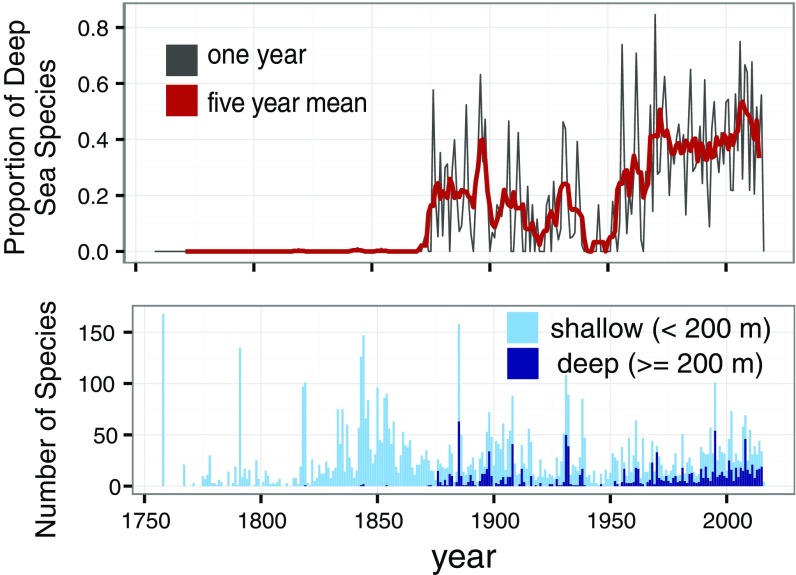
The description model and its associated forecasts are also useful tools for comparisons of clade diversity. In the marine system, deep-sea exploration has dramatically elevated our estimates of species diversity in many groups (29), and we estimate that 43% of marine bivalve species described since 2005 were discovered in the deep sea (Fig. S9) (30). Thus, newly discovered species may be concentrated within particular clades, which may challenge the interpretation of many ecological and evolutionary patterns derived from strictly continental shelf occurrences (31).

Fig. S9.

(Top) Proportion of bivalve species described from the deep sea per year. (Bottom) Actual counts of species described in the deep sea and continental shelf per year. For the last 50 years, approximately 40% of newly described species were discovered in the deep sea.

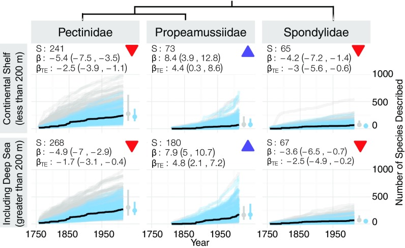
Including newly discovered deep-sea species changes the relative richness of three well-studied, monophyletic bivalve families. When only considering continental shelf species (water depths of <200 m), true scallops (Pectinidae) are nearly 3 times as diverse as their closest relatives, the mainly tropical thorny oysters (Spondylidae) and the cold-water glass scallops (Propeamussiidae). However, recent deep-sea discoveries (e.g., ref. 32) have more than doubled the number of glass scallops, bringing their diversity much closer to that of their sister clade, the true scallops (Fig. 4). Still, even with their apparent taxonomic undersaturation, we do not predict the glass scallops to surpass or even match the diversity of the mainly continental shelf true scallops for the next 20 and 50 y (Table S2).

Fig. 4.

Description of three closely related clades of marine bivalves excluding and including deep-sea species (phylogeny from ref. 33). Panels are organized as in Fig. 2. Despite the doubling of diversity in Propeamussiidae when including deep-sea species, these glass scallops are not forecast to overtake the diversity of their more speciose sister clade Pectinidae—the true scallops.

Table S2.

Twenty- and 50-y forecasts of species richness within clades across model fits with and without TE

Bivalve family	2016 richness	2035 noTE	2035 TE	2065 noTE	2065 TE
Continental shelf only
Pectinidae	241	261 (249 to 291)	257 (249 to 272)	263 (263 to 331)	293 (268 to 313)
Propeamussiidae	69	73 (71 to 78)	75 (71 to 85)	83 (77 to 85)	77 (73 to 79)
Spondylidae	65	70 (65 to 80)	68 (66 to 74)	77 (73 to 103)	77 (75 to 85)
Including deep sea
Pectinidae	268	289 (276 to 317)	285 (277 to 299)	320 (302 to 364)	337 (323 to 421)
Propeamussiidae	176	189 (185 to 197)	197 (188 to 223)	200 (195 to 208)	202 (200 to 252)
Spondylidae	67	72 (67 to 81)	70 (67 to 76)	82 (79 to 110)	73 (71 to 75)

Values in the 2035 or 2065 columns are the median forecast species richness for that year, with the 80% credible interval in parentheses.

These probable estimates of clade diversity raise questions about the relationship between each clade’s richness and biological or environmental factors. At least within these three families, bathymetric affinity alone appears to be a poor predictor of species richness. Instead, the greater ecological breadth of the true scallops may explain their higher diversity over the more restricted ecology of the mostly carnivorous glass scallops and sessile, filter-feeding thorny oysters. Estimating the probability of diversity shifts among clades with continued description of deep-sea species will be paramount for correctly interpreting evolutionary patterns.

Improving Estimates of Species Richness.

Alternative estimates of TE.

Estimating true TE will require negative evidence, that is, the failure to recognize new species after repeated attempts. Combining recent region- and clade-specific faunal inventories can offer unparalleled insight into the taxonomic stability and saturation of the taxonomic record. In marine bivalves, recent rigorous molecular and morphological examination of a chemosybiotic group (Lucinidae) from Panglao, Philippines, in the Tropical West Pacific confirmed 50 existing species and discovered 26 new species (34); a similar treatment of lucinids from Guadeloupe in the TWA confirmed 25 existing and 1 new species (35). Despite all of the potential biases conflating the results of our model, these observed descriptions are precisely the dynamic that our model and other models (36) predict for the undiscovered diversity within these two regions.

Trends in biological characteristics.

As the clade analysis shows, the biological properties of organisms can strongly affect the timing of the discovery and description of new species (8, 25). The earliest descriptions within many marine groups are commonly of species with larger body sizes, larger geographic ranges, and shallower bathymetric occurrences (37, 38). As the model stands here, we interpret a region or a clade with a relatively strong decline in species description rate as being closer to taxonomic saturation. However, if the body sizes and geographic range sizes of the species within that region show a temporally constant or increasing trend over time, we might conclude that the observed richness is unsaturated, because those species most easily encountered by systematists are still being described (39, 40). The challenge remains to directly incorporate these biological trends into a spatially and taxonomically explicit probabilistic model of species discovery.

Accounting for invalid descriptions.

We modeled the description of currently accepted species and thus assumed the observed taxonomic record is completely stable. However, taxonomic revision on both morphological and molecular grounds can split (add) and synonymize (remove) species throughout the history of description. Reshaping the description curve changes the inferred rates of long-term description and the subsequent forecast of undiscovered species.

The history of taxonomic practice within a particular clade provides qualitative insight into the stability of an observed description curve. Most marine bivalve species have been defined by their morphology, and recent molecular work largely supports these lower-level taxonomic delimitations (22, 41). This general agreement between morphology and molecules reduces the likelihood of extensive synonymies or adding a large number of morphologically cryptic species. Cryptic species certainly exist, but their influence on the description curve is difficult to predict. Systematists reinstate an older, synonymized name (e.g., from year 1850) for a newly verified genetic unit or apply a new name entirely (e.g., in year 2017). Reinstatement of older names will produce stronger declines in the long-term trend of description, suggesting higher taxonomic saturation. Applying new names will contribute to a rise in long-term description rates, implying lower taxonomic saturation. Given the general congruency between molecules and morphology in bivalves, we expect most synonymized older names to remain synonymized and changes to the shape of the description curve to come primarily from new species descriptions.

Higher taxonomic groups such as birds, mammals, and bivalves are unlikely to exhibit similar histories of taxonomic revision, making the qualitative tactic above impractical for studying broad patterns in comparative biology (e.g., ref. 42). The net species description rate is the sum of the synonymization rate (reduce accepted species) and reinstatement rate (increase accepted species). Thus, in a given year, the probability of observing the currently accepted number of species is a function of the long- and short-term trends in description rate and the rate at which species are deemed invalid. Alternatively, the persistence of a species name could be modeled as a birth–death-type process in an extension of the “flux rate” method (43). Either proposed framework would provide the most probable “net taxonomic output” for a given year.

Comparing the idiosyncrasies of system-specific taxonomic records will be very important for designing and testing general models of species discovery. Removing the effects of taxonomic culture will always be difficult in comparative studies of higher taxonomic groups, but modeling the dynamics of description loss and reinstatement is likely the most promising method for future development.

Conclusions

Comparative macroecological and macroevolutionary studies often treat observed richness as known, but failing to account for the spatial and phylogenetic variation in taxonomic activity may mislead interpretations of biodiversity dynamics derived from currently observed species richness. Modeling the long-term species description rate provides a direct comparison of taxonomic knowledge among geographic regions or clades. Incorporating those trends and their associated uncertainties into short-term forecasts of species richness generates a set of probable values, which can be directly used in quantitative ecological and evolutionary models and in assessing the knowledge of diversity in and around biological reserves. Integrating description rates with forecasts of species richness not only improves our interpretations of current biodiversity patterns but also highlights areas where continued systematic research and discovery is necessary for building more rigorous quantitative analyses at higher spatial and phylogenetic resolution.

Materials and Methods

Marine Bivalve Database.

Our marine bivalve database includes 5,744 currently valid species with 62,059 georeferenced occurrences (44) (Dataset S1). For the regional richness study, we focus on intertidal to continental shelf bivalves (living at depths from 0 m to 200 m), as deep-sea bivalves are widely acknowledged to be an independent and undersampled system (45). We also exclude two clades of exceptionally small body size (<1 cm) that have poorly understood taxonomy [Cyamioidea and Galeommatoidea (21, 30, 46)]. For the clade study, we include taxonomically standardized deep-sea occurrences from a low-resolution taxonomic dataset of 136 deep-sea species (largely from ref. 30; Dataset S2).

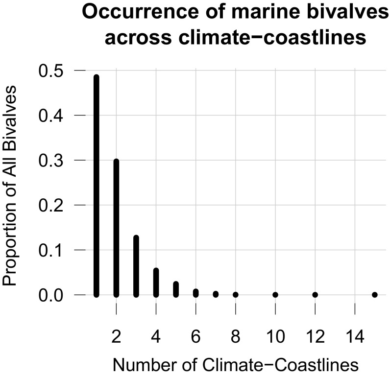
We define 18 geographic regions termed “climate–coastlines” using a combination of coastline geography, climate zones, and major biogeographic turnover (map in Fig. 2) (47). Our climate–coastlines resemble the 12 “realms” in the Marine Ecoregions of the World (48), but we split the realms by coastline to reflect the biogeographic structure of shelf biotas. We assigned species to one or more climate–coastlines by intersecting the individual occurrences for each species with the climate–coastline boundaries. Approximately 48% of species are endemic to one climate–coastline, and ∼40% of species occur across two and three climate–coastlines (Fig. S10). Allowing species to occur across more than one climate–coastline makes the regional description histories more similar, which biases against the test for differences in description history.

Fig. S10.

Proportion of bivalves occurring in climate–coastlines. Approximately 50% of bivalve species occur in only one or two climate–coastlines. A combined 92% of bivalve species occur in three or fewer climate–coastlines. Only around 8%, or ∼500 species, of bivalves could be considered widespread in that they occur across four or more climate–coastlines.

Modeling Species Description.

We generate the number of species described in a given year following a zero-inflated Poisson distribution (49). Zero inflation accommodates an excess of individual years having zero description events above that expected under a Poisson distribution—a common characteristic of regional and clade description curves. We modified the zero-inflation component to allow for long runs of consecutive years with zero species described by modeling the occurrence probability of a description event as a two-state Markov chain. We characterize the long-term temporal trend in species description series using an autoregressive conditional Poisson regression (50). Within this regression, the predicted number of species described per year is a function of time and the long-term and short-term autoregressive components of the description rate. Finally, we incorporated TE, defined here as the number of unique publications describing new bivalve species for a given year, as an offset term for the number of species named per year (51). Including TE in the model transforms the interpretation of the estimated parameters from the expected number of species described per year to the rate of species described per publication per year. Full model description, formulation, and choice of priors is in Supporting Information, and model code is available from Zenodo (doi.org/10.5281/zenodo.159033).

The joint posterior of our model parameters was estimated using a variant of Hamiltonian Monte Carlo called the No U-Turn Sampler, as implemented in the probabilistic programing language Stan (52). Four independent chains were run for 15,000 steps each (5,000 warm-up) and were well mixed [$\widehat{R}=\mathrm{\hspace{0.17em}1}$ (52)]. Model adequacy was assessed using posterior predictive simulations to determine whether patterns generated from the parameter estimates resemble the empirically observed patterns—the fundamental determinant of model fit. We made 1,000 independent draws from the marginal posterior distributions of each parameter and compared these posterior estimates to the observed patterns of taxonomic discovery through graphical comparisons (Fig. 2).

Forecasting Species Richness.

We forecast species richness across groups (regions and clades) by simulating forward in time from the posterior predictive distribution. We examined the forecasting error using a variant of leave-p-out time series cross-validation [“rolling forecast origin” (53), recommended in ref. 4], where we fit the model to incremental time series from k blocks of p years each starting with 1758–1765. For $p=\mathrm{\hspace{0.17em}5}$, the series is 1758–1765, 1758–1770,…, 1758–2010. We estimated the species richness p years into the future for each block by drawing parameter estimates from the model posterior (for the TE model, we used random samples of publication counts p years before the end of the time series). We estimated the forecasting error as the difference between the observed and forecast counts within a forecast window (Fig. S7).

Formal Model Definition

We analyze the record of species named per analytical group (e.g., biogeographic region) as a hierarchical Bayesian model (20). There are $J$ groups where $j=\mathrm{\hspace{0.17em}1},2,\mathrm{\dots },J$. Each group has a specific time series of species named per year $y^j$ (minimum 0) with length $T^j$, which is the number of years between the first year a species was described in a group $j$ and the last year.

We model $y^j$ as a zero-inflated Poisson regression where the Poisson distribution follows an autoregressive conditional Poisson model (ACP) and the Bernoulli distribution follows a two-state Markov model (Eq. S1 and refs. 50 and 51, following formulation in ref. 55):

$$p(y_t^j|{\theta }^j,{\lambda }_t^j)=\{\begin{array}{cc}{\theta }_t^j+(1-{\theta }_t^j)\times \mathrm{Pois}(0|(u_t^j+1){\lambda }_t^j)\hfill & \text{if}\hspace{0.17em}{y}_t^j=0,\text{and}\hfill \\ (1-{\theta }_t^j)\times \mathrm{Pois}(y_t^j|{\lambda }_t^j)\hfill & \text{if}\hspace{0.17em}{y}_t^j>0,\hfill \end{array}$$ [S1]

where ${\theta }_t^j$ is the probability for region $j$ at time $t$ that $y_t^j$ equals 0, and $1-{\theta }_t^j$ is the probability that $y_t^j$ is a draw from a Poisson distribution with rate ${\lambda }_t^j$ (Eq. S3); $u_t^j$ is the number of publications necessary to name $y_t^j$ species plus 1, because the Poisson rate is undefined at 0.

Here ${\theta }^j$ is a length $T^j$ vector whose elements are modeled as a two-state Markov process (Eq. S2; this accounts for possible long runs of no species being named. The probability for region $j$ that $y_t^j=\mathrm{\hspace{0.17em}0}|y_{t-1}^j=\mathrm{\hspace{0.17em}0}$ is ${\gamma }^j$, and ${\eta }^j$ is the probability for region $j$ that $y_t^j\ne 0|y_{t-1}^j=\mathrm{\hspace{0.17em}0}$; $z^j$ is then a length $T$ indicator vector where $z_t^j=\mathrm{\hspace{0.17em}0}$ if $y_t^j=\mathrm{\hspace{0.17em}0}$ and $z_t^j=\mathrm{\hspace{0.17em}1}$ if $y_t^j\ne \mathrm{\hspace{0.17em}0}$:

$$\begin{array}{c}{\theta }_t^j=z_t^j{\gamma }^j+(1-z_t){\eta }^j\\ {\gamma }^j\sim \mathrm{U}(\mathrm{0,1})\\ {\eta }^j\sim \mathrm{U}(\mathrm{0,1}).\end{array}$$ [S2]

We use an ACP regression to account for the temporal autocorrelation present in the time series, where ${\lambda }^j$ is a length $T^j$ vector of Poisson rates (Eq. S3). The short-term autocorrelation in number named ${\alpha }_j$ is the number of species named at time $t-1$, and the long-term autocorrelation in rate ${\beta }_j$ is the value of ${\lambda }^j$ at time $t-1$. Both ${\alpha }_j$ and ${\beta }_j$ are constrained to be between 0 and 1 so that ${\alpha }_j+{\beta }_j\le 1$. These parameters are given independent uniform priors; ${\alpha }_j$ and ${\beta }_j$ are not defined for the first time point, so, when $t=1$, these terms are not included (Eq. S3). Thus, the ACP part of the mixture model is defined as:

$$\begin{array}{c}{\lambda }_t^j=\{\begin{array}{cc}{\varphi }_j\hspace{1em}\hfill & \text{if}\hspace{0.17em}t=1,\text{and}\hfill \\ {\omega }_t^j+{\alpha }_j{y}_{t-1}^j+{\beta }_j{\lambda }_{t-1}\hspace{1em}\hfill & \text{if}\hspace{0.17em}t>1\hfill \end{array}\hfill \\ {\varphi }_j\sim \log N({\mu }_{\varphi },{\sigma }_{\varphi })\\ {\mu }_{\varphi }\sim N(\mathrm{0,1})\\ {\sigma }_{\varphi }\sim {\mathrm{C}}^{+}(1)\\ {\alpha }_j\sim \mathrm{U}(\mathrm{0,1})\\ {\beta }_j\sim \mathrm{U}(0,1-{\alpha }_j).\end{array}$$ [S3]

Increased temporal autocorrelation can be modeled by adding lags. In that case, ${\lambda }_t^j$ would be defined as ${\lambda }_t^j={\omega }_t^j+({\sum }_{k=1}^K{\alpha }_{j,k}{y}_{t-1}^j)+({\sum }_{k=1}^K{\beta }_{j,k}{\lambda }_{t-1,k})$, where $K=$ number of lags and ${\alpha }_{j,k}+{\beta }_{j,k}\le 1$.

The expected number of species in group $j$ named in the first year (t = 1) is ${\varphi }_j$; ${\varphi }_j$ is considered a realization from the shared distribution of species named in the first year and was assumed to be log-normally distributed with log-mean ${\mu }_{\varphi }$ and log-scale ${\sigma }_{\varphi }$, which were both given weakly informative priors.

The intercept of the ACP regression ${\omega }^j$ is modeled as a hierarchical linear model, also known as a generalized linear mixed effect model (20) with a log-link function (Eq. S4). $X$ is a $T\times 2$ matrix of predictors, where $T$ is the number of years since the first species was identified. The first column of $X$ corresponds to the intercept term (all set to 1), and the second column is the year corresponding to that row; $\delta$ is a $2\times J$ matrix of regression coefficients, where J is the number of regions in the study.

The matrix of correlation coefficients $\delta$ is given a multivariate normal prior with mean vector $\mu$ of length D and covariance matrix $\mathrm{\Sigma }$, which is $D\times D$. The elements of $\mu$ correspond to the overall average intercept and slope terms, where the slopes correspond to the temporal trend and are given independent normally distributed priors. $\mathrm{\Sigma }$ is decomposed into a length two vector of scales $\tau$ and a $2\times 2$ correlation matrix $\mathrm{\Omega }$. The elements of $\tau$ are given independent half-Cauchy priors, and $\mathrm{\Omega }$ is given a prior from the Lewandowski, Kurowicka, and Joe (LKJ) Correlation Distribution, following the Stan manual (54). Here $\mu$ represents the average values of $\delta$ across all biogeographic regions, $\tau$ are the standard deviations of the region-specific estimates ${\delta }_j$, and $\mathrm{\Omega }$ is the correlation between the intercept and slope terms of $\delta$ as they vary by region.

$$\begin{array}{c}{\omega }_t=\exp (X_t{\delta }_j)\\ \delta \sim \mathrm{MVN}(\mu ,\mathrm{\Sigma })\\ \mathrm{\Sigma }=\text{diag}(\tau )\mathrm{\Omega }\text{diag}(\tau )\\ \mathrm{\Omega }\sim \mathrm{LKJ}(2)\\ {\tau }_j\sim {\mathrm{C}}^{+}(1).\end{array}$$ [S4]

Full model code is available from Zenodo (doi.org/10.5281/zenodo.159033).

References

- 1.Hey J, Waples RS, Arnold ML, Butlin RK, Harrison RG. Understanding and confronting species uncertainty in biology and conservation. Trends Ecol Evol. 2003;18(11):597–603. [Google Scholar]
- 2.McPeek MA. The ecological dynamics of clade diversification and community assembly. Am Nat. 2008;172(6):270–284. doi: 10.1086/593137. [DOI] [PubMed] [Google Scholar]
- 3.Isaac NJB, Purvis A. The ‘species problem’ and testing macroevolutionary hypotheses. Divers Distrib. 2004;10(4):275–281. [Google Scholar]
- 4.Wilson SP, Costello MJ. Predicting future discoveries of European marine species by using a non-homogeneous renewal process. J R Stat Soc Ser C Appl Stat. 2005;54(5):897–918. [Google Scholar]
- 5.May RM. Tropical arthropod species, more or less? Science. 2010;329(5987):41–42. doi: 10.1126/science.1191058. [DOI] [PubMed] [Google Scholar]
- 6.Price T. The debate on determinants of species richness. Am Nat. 2015;185(5):571. doi: 10.1086/680858. [DOI] [PubMed] [Google Scholar]
- 7.Meijaard E, Nijman V. Primate hotspots on Borneo: Predictive value for general biodiversity and the effects of taxonomy. Conserv Biol. 2003;17(3):725–732. [Google Scholar]
- 8.May RM. How many species are there on Earth? Science. 1988;241:1441–1449. doi: 10.1126/science.241.4872.1441. [DOI] [PubMed] [Google Scholar]
- 9.Patterson BD. Accumulating knowledge on the dimensions of biodiversity: Systematic perspectives on Neotropical mammals. Biodiv Lett. 1994;2(3):79–86. [Google Scholar]
- 10.Solow AR, Smith WK. On estimating the number of species from the discovery record. Proc Bio Sci. 2005;272(1560):285–287. doi: 10.1098/rspb.2004.2955. [DOI] [PMC free article] [PubMed] [Google Scholar]
- 11.Bebber DP, Marriott FHC, Gaston KJ, Harriss SA, Scotland RW. Predicting unknown species numbers using discovery curves. Proc Bio Sci. 2007;274(1618):1651–1658. doi: 10.1098/rspb.2007.0464. [DOI] [PMC free article] [PubMed] [Google Scholar]
- 12.Joppa LN, Roberts DL, Pimm SL. How many species of flowering plants are there? Proc Bio Sci. 2011;278(1705):554–559. doi: 10.1098/rspb.2010.1004. [DOI] [PMC free article] [PubMed] [Google Scholar]
- 13.Caley MJ, Fisher R, Mengersen K. Global species richness estimates have not converged. Trends Ecol Evol. 2014;29(4):187–188. doi: 10.1016/j.tree.2014.02.002. [DOI] [PubMed] [Google Scholar]
- 14.Linnaeus C. Systema Naturæ per Regna Tria Naturæ, Secundum Classes, Ordines, Genera, Species, cum Characteribus, Differentiis, Synonymis, Locis. 10th Ed. Impensis Direct. Laurentii Salvii; Stockholm: 1758. Latin. [Google Scholar]
- 15.Appeltans W, et al. The magnitude of global marine species diversity. Curr Biol. 2012;22(23):2189–2202. doi: 10.1016/j.cub.2012.09.036. [DOI] [PubMed] [Google Scholar]
- 16.Joppa LN, Roberts DL, Myers N, Pimm SL. Biodiversity hotspots house most undiscovered plant species. Proc Natl Acad Sci USA. 2011;108(32):13171–13176. doi: 10.1073/pnas.1109389108. [DOI] [PMC free article] [PubMed] [Google Scholar]
- 17.Costello MJ, Wilson S, Houlding B. Predicting total global species richness using rates of species description and estimates of taxonomic effort. Syst Biol. 2012;61(5):871–883. doi: 10.1093/sysbio/syr080. [DOI] [PubMed] [Google Scholar]
- 18.Costello MJ, Wilson S, Houlding B. More taxonomists describing significantly fewer species per unit effort may indicate that most species have been discovered. Syst Biol. 2013;62(4):616–624. doi: 10.1093/sysbio/syt024. [DOI] [PubMed] [Google Scholar]
- 19.Sangster G, Luksenburg JA. Declining rates of species described per taxonomist: Slowdown of progress or a side-effect of improved quality in taxonomy? Syst Biol. 2015;64(1):144–151. doi: 10.1093/sysbio/syu069. [DOI] [PubMed] [Google Scholar]
- 20.Gelman A, et al. Bayesian Data Analysis. Chapman & Hall; Boca Raton, FL: 2013. [Google Scholar]
- 21.Bieler R, Mikkelsen PM, Giribet G. Bivalvia–A discussion of known unknowns. Am Malacol Bull. 2013;31(1):123–133. [Google Scholar]
- 22.Mikkelsen PM. Speciation in modern marine Bivalves (Mollusca: Bivalvia): Insights from the published record. Am Malacol Bull. 2011;29(1-2):217–245. [Google Scholar]
- 23.Bouchet P, Lozouet P, Maestrati P, Heros V. Assessing the magnitude of species richness in tropical marine environments: Exceptionally high numbers of molluscs at a New Caledonia site. Biol J Linn Soc. 2002;75(1996):421–436. [Google Scholar]
- 24.Isaac NJB, Mallet J, Mace GM. Taxonomic inflation: Its influence on macroecology and conservation. Trends Ecol Evol. 2004;19(9):464–469. doi: 10.1016/j.tree.2004.06.004. [DOI] [PubMed] [Google Scholar]
- 25.Scheffers BR, Joppa LN, Pimm SL, Laurance WF. What we know and don’t know about Earth’s missing biodiversity. Trends Ecol Evol. 2012;27(9):501–510. doi: 10.1016/j.tree.2012.05.008. [DOI] [PubMed] [Google Scholar]
- 26.Gray A, Cavers S. Island biogeography, the effects of taxonomic effort and the importance of island niche diversity to single-island endemic species. Syst Biol. 2014;63(1):55–65. doi: 10.1093/sysbio/syt060. [DOI] [PubMed] [Google Scholar]
- 27.Jackson JBC, Jung P, Coates AG, Collins LS. Diversity and extinction of tropical American mollusks and emergence of the Isthmus of Panama. Science. 1993;260(5114):1624–1626. doi: 10.1126/science.260.5114.1624. [DOI] [PubMed] [Google Scholar]
- 28.Allmon WD, Rosenberg G, Portell RW, Schindler KS. Diversity of Atlantic coastal-plain mollusks since the Pliocene. Science. 1993;260(5114):1626–1629. doi: 10.1126/science.260.5114.1626. [DOI] [PubMed] [Google Scholar]
- 29.Rex MA, Etter RJ. Deep-Sea Biodiversity. Harvard Univ Press; Cambridge, MA: 2010. [Google Scholar]
- 30.Huber M. Compendium of Bivalves II. ConchBooks; Hackenheim, Germany: 2015. [Google Scholar]
- 31.Woolley SNC, et al. Deep-sea diversity patterns are shaped by energy availability. Nature. 2016;533(7603):393–396. doi: 10.1038/nature17937. [DOI] [PubMed] [Google Scholar]
- 32.Dijkstra HA, Maestrati P. New species and new records of deep-water Pectinoidea (Bivalvia: Propeamussiidae, Entoliidae and Pectinidae) from the South Pacific. Mem Mus Natl Hist Nat. 2008;196:77–113. [Google Scholar]
- 33.Bieler R, et al. Investigating the bivalve tree of life – an exemplar-based approach combining molecular and novel morphological characters. Invertebr Syst. 2014;28(1):32–115. [Google Scholar]
- 34.Glover EA, Taylor JD. Lucinidae of the Philippines: Highest known diversity and ubiquity of chemosymbiotic bivalves from intertidal to bathyal depths (Mollusca: Bivalvia) Mem Mus Natl Hist Nat. 2016;208:65–234. [Google Scholar]
- 35.Taylor JD, Glover EA. Lucinid bivalves of Guadeloupe: Diversity & systematics in the context of the tropical Western Atlantic (Mollusca: Bivalvia: Lucinidae) Zootaxa. 2016;4196(3):301–380. doi: 10.11646/zootaxa.4196.3.1. [DOI] [PubMed] [Google Scholar]
- 36.Bouchet P, Bary S, Héros V, Marani G. How many species of molluscs are there in the world’s oceans, and who is going to describe them? In: Héros V, Strong E, Bouchet P, editors. Tropical Deep-Sea Benthos Mémoires du Muséum National d’Histoire Naturelle. Vol 29. Mus Natl Hist Nat; Paris: 2016. pp. 9–24. [Google Scholar]
- 37.Gibbons MJ, et al. What determines the likelihood of species discovery in marine holozooplankton: Is size, range or depth important? Oikos. 2005;109(3):567–576. [Google Scholar]
- 38.Costello MJ, Lane M, Wilson S, Houlding B. Factors influencing when species are first named and estimating global species richness. Glob Ecol Conserv. 2015;4:243–254. [Google Scholar]
- 39.Adamowicz SJ, Purvis A. How many branchiopod crustacean species are there? Quantifying the components of underestimation. Glob Ecol Biogeogr. 2005;14(5):455–468. [Google Scholar]
- 40.Stork NE, McBroom J, Gely C, Hamilton AJ. New approaches narrow global species estimates for beetles, insects, and terrestrial arthropods. Proc Natl Acad Sci USA. 2015;112(24):7519–7523. doi: 10.1073/pnas.1502408112. [DOI] [PMC free article] [PubMed] [Google Scholar]
- 41.Jablonski D, Finarelli JA. Congruence of morphologically-defined genera with molecular phylogenies. Proc Natl Acad Sci USA. 2009;106(20):8262–8266. doi: 10.1073/pnas.0902973106. [DOI] [PMC free article] [PubMed] [Google Scholar]
- 42.Tomašových A, et al. Unifying latitudinal gradients in range size and richness across marine and terrestrial systems. Proc Bio Sci. 2016;283(1830):20153027. doi: 10.1098/rspb.2015.3027. [DOI] [PMC free article] [PubMed] [Google Scholar]
- 43.Alroy J. How many named species are valid? Proc Natl Acad Sci USA. 2002;99(6):3706–3711. doi: 10.1073/pnas.062691099. [DOI] [PMC free article] [PubMed] [Google Scholar]
- 44.Jablonski D, et al. Out of the tropics, but how? Fossils, bridge species, and thermal ranges in the dynamics of the marine latitudinal diversity gradient. Proc Natl Acad Sci USA. 2013;110(26):10467–10469. doi: 10.1073/pnas.1308997110. [DOI] [PMC free article] [PubMed] [Google Scholar]
- 45.Valentine JW, Jablonski D. A twofold role for global energy gradients in marine biodiversity trends. J Biogeogr. 2015;42(6):997–1005. [Google Scholar]
- 46.Valentine JW, Jablonski D, Kidwell S, Roy K. Assessing the fidelity of the fossil record by using marine bivalves. Proc Natl Acad Sci USA. 2006;103(17):6599–6604. doi: 10.1073/pnas.0601264103. [DOI] [PMC free article] [PubMed] [Google Scholar]
- 47.Belanger CL, et al. Global environmental predictors of benthic marine biogeographic structure. Proc Natl Acad Sci USA. 2012;109(35):14046–14051. doi: 10.1073/pnas.1212381109. [DOI] [PMC free article] [PubMed] [Google Scholar]
- 48.Spalding MD, et al. Marine ecoregions of the world: A bioregionalization of coastal and shelf areas. Bioscience. 2007;57(7):573–583. [Google Scholar]
- 49.Lambert D. Zero-inflated Poisson regression, with an application to defects in manufacturing. Technometrics. 1992;34(1):1–14. [Google Scholar]
- 50.Fokianos K, Rahbek A, Tjøstheim D. Poisson autoregression. J Am Stat Assoc. 2009;104(488):1430–1439. [Google Scholar]
- 51.Gelman A, Hill J. Data Analysis Using Regression and Multilevel/Hierarchical Models. Cambridge Univ Press; Cambridge, UK: 2007. [Google Scholar]
- 52.Carpenter B, et al. Stan: A probabilistic programming language. J Stat Softw. 2017;76(1):1–32. doi: 10.18637/jss.v076.i01. [DOI] [PMC free article] [PubMed] [Google Scholar]
- 53.Hyndman RJ, Athanasopoulos G. 2013 Forecasting: Principles & Practice. Available at https://www.otexts.org/fpp. Accessed September 27, 2016.
- 54.Stan Development Team 2016 Stan Modeling Language Users Guide and Reference Manual, Version 2.9.0. Available at mc-stan.org. Accessed September 21, 2016.
Associated Data
This section collects any data citations, data availability statements, or supplementary materials included in this article.