Bayesian prediction of RNA translation from ribosome profiling

Abstract

Ribosome profiling via high-throughput sequencing (ribo-seq) is a promising new technique for characterizing the occupancy of ribosomes on messenger RNA (mRNA) at base-pair resolution. The ribosome is responsible for translating mRNA into proteins, so information about its occupancy offers a detailed view of ribosome density and position which could be used to discover new translated open reading frames (ORFs), among other things. In this work, we propose Rp-Bp, an unsupervised Bayesian approach to predict translated ORFs from ribosome profiles. We use state-of-the-art Markov chain Monte Carlo techniques to estimate posterior distributions of the likelihood of translation of each ORF. Hence, an important feature of Rp-Bp is its ability to incorporate and propagate uncertainty in the prediction process. A second novel contribution is automatic Bayesian selection of read lengths and ribosome P-site offsets (BPPS). We empirically demonstrate that our read length selection technique modestly improves sensitivity by identifying more canonical and non-canonical ORFs. Proteomics- and quantitative translation initiation sequencing-based validation verifies the high quality of all of the predictions. Experimental comparison shows that Rp-Bp results in more peptide identifications and proteomics-validated ORF predictions compared to another recent tool for translation prediction.

INTRODUCTION

Ribosome profiling via high-throughput sequencing (ribo-seq, (1)) is a promising new experimental technique for identifying the position of ribosomes on messenger RNA (mRNA). Several ribosome profiling protocols have been developed. For example, Aeschimann et al. (2) lyse cells, digest the lysate with RNAseI and purify the monosomes via sucrose gradient fractionation or gel filtration. RNA is then isolated from the monosome fraction, subjected to gel purification and size selection to enrich for mRNA fragments of interest, so-called ribosome footprints. The ribosome footprints are then amplified, sequenced and mapped to a genome. We call the pattern of mapped reads for a particular region (e.g. an open reading frame (ORF)) as the region's ribosome profile, or just profile.

Ideally, the ribosome profile reveals exactly and only the position of ribosomes. In practice, though, a variety of other signals and noise (1), such as RNAs protected by complexes other than the ribosome, amplification biases and sequencing errors, dilute the ribosome profile signal. Furthermore, some evidence suggests that the ribosome can bind to mRNA (and protect it) without actively translating (3).

The ribosome has known behavior which can help distinguish noise from true signal in ribosome profiles (1). In particular, the ribosome respects the genetic code and moves along its RNA template during protein synthesis in steps of 3-nt (i.e. size of a codon). Thus, the true signal of an actively translated mRNA transcript should exhibit a periodic ‘high-low-low’ behavior in which every third base pair has more ribosome footprints than the surrounding base pairs. (While other patterns, such as ‘high-low-high,’ are also periodic, we specifically refer to the ‘high-low-low’ pattern with respect to a specific starting point as periodic.)

Related work

A variety of techniques have been proposed for analyzing ribo-seq data. Many focus on translational efficiency (4); for example, regression models (5,6) have been used to detect differences in ribo-seq expression which is not explained by matching RNA-seq measurements.

Ribosome profiling has also been used to study translational dynamics. For example, Gritsenko et al. (7) estimated translation initiation and elongation rates with ribo-seq. In particular, classic assumptions of tRNA concentrations and elongation rates have been called into question as a result of analysis with ribo-seq data (8). However, further analysis (9,10) suggests that variations in protocols significantly affect these estimates.

Recent work (11,12) has shown that using unannotated ORFs supported by ribo-seq improves downstream proteomics analysis.

The ribosome release score (3), which is a normalized ratio of reads within an ORF and its transcript trailer, is an early approach for distinguishing translated and untranslated ORFs. The ORFscore (13) for classifying ORFs is based on the amount by which in-frame reads exceed those in other reading frames; conceptually, ORFscore is quite similar to a χ² test.

ORF-RATER (14) extracts characteristics from annotated protein-coding transcripts to train a random forest classifier; the classifier is then used to label unannotated ORFs. It uses linear regression to account for overlapping ORFs. Recently, a hidden Markov model-based approach, riboHMM (15), was proposed to handle the variance inherent in ribo-seq profiles; however, riboHMM requires ad hoc approaches to identify more than one translated ORF for each transcript. Both ORF-RATER and riboHMM are supervised prediction approaches; that is, they require example ORFs a priori labeled as ‘translated’ for training. Thus, these approaches are implicitly biased toward identifying new ORFs similar to the ones selected for training.

A recent unsupervised approach, RiboTaper (16), uses multitapers to identify ORFs which exhibit 3-nt periodicity. RiboTaper is the current state of the art and falls into the same domain as Rp-Bp. That is why, we include a comparison with RiboTaper in the ‘Results’ section.

As we discuss in more detail in ‘Materials and Methods’ section, our approach automatically determines periodic read lengths and P-site offsets. The recent RiboProfiling (17) package also does this; however, Rp-Bp uses a principled model selection approach to identify only periodic read lengths and their offsets. Furthermore, Rp-Bp allows distinct P-site offsets for each read length.

Contribution

In this work, we propose an unsupervised Bayesian approach, called Ribosome profiling with Bayesian predictions, Rp-Bp, which takes advantage of the ribosome's periodic behavior to identify translated ORFs based on ribosome profiles. That is, we look for a ‘high-low-low’ pattern in the profiles. By design, Rp-Bp naturally identifies all translated ORFs which exhibit this pattern, regardless of how many fall on the same transcript.

Conceptually, we capture the periodic behavior using a two-component mixture model. The first component models in-frame ribo-seq signal, which is expected to be high for actively translating ribosomes. The other component enforces periodicity by ensuring that the out-of-frame signal is lower.

The prediction pipeline consists of two phases. It first constructs a profile for each ORF from ribo-seq reads. This phase uses a number of filters to ensure high quality of the profile. We propose a novel probabilistic approach for automatically selecting periodic ribo-seq read lengths and their P-site offsets. Our results show that this automated technique results in modestly more canonical and non-canonical predicted ORFs than manual selection by an expert; the numbers of variants and out-of-frame predicted ORFs remain similar. Importantly, this selection does not require manual intervention, so it is easily integrated into analysis pipelines.

The second phase entails the prediction of ORF translation from the profiles using a different variant of the two-component mixture model. A Bayesian model selection approach is again used to explicitly incorporate and propagate uncertainty in the inference process. Our experimental analysis verifies the accuracy of these predictions using proteomics and an alternative sequencing approach for identifying translation quantitative translation initiation sequencing (QTI-seq, (18)). Our results also show that Rp-Bp results in more peptide identifications and ORFs with proteomics validation than RiboTaper.

MATERIALS AND METHODS

Our Bayesian approach for translation prediction, called Ribosome profiling with Bayesian predictions, Rp-Bp, consists of two phases: ORF profile construction (Figure 1) and translation prediction (Figure 2).

Figure 1.

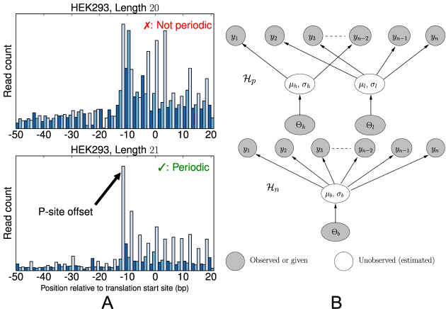
(A) Metagene profiles from a HEK293 dataset for reads with length 20 bp (top) and 21 bp (bottom). The reads of length 21 bp show a clear 3-nt periodicity, while those of length 20 bp do not. (B) Simplified view of graphical models for estimating the periodicity of metagene profiles. (Top) The periodic model, H_p, is a two-component mixture model in which the count of the first nucleotide of each codon is drawn from a ‘high’ component h while the other two nucleotides’ counts in the codon are drawn from a ‘low’ component l. That is, this model fits the ‘high-low-low’ pattern of translating ribosomes. (Bottom) The non-periodic model, H_n, is a naïve Bayes model in which all nucleotide counts are drawn from the same distribution.

Figure 2.

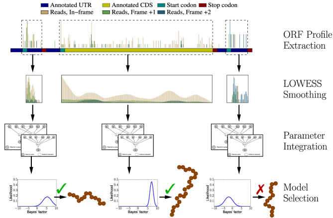
The translation prediction workflow. For each identified ORF, posterior likelihoods of and are estimated from its smoothed profile using Hamiltonian Markov chain Monte Carlo. The posterior distribution of the Bayes factor is calculated (in closed form) from these estimates. The posterior Bayes factor distribution are used to label each ORF as ‘translated’ (✓) or ‘untranslated’ (✗).

The ribo-seq ORF profiles are, by design, non-negative integers because they are based on counts. Nevertheless, we model these values with unbounded continuous distributions (Gaussian and Cauchy) in all of the graphical models which follow. As discussed below, we use a smoothing strategy which converts the counts into continuous values. Thus, count-based distributions, such as the negative binomial, are not appropriate in this context. Furthermore, this allows our models to directly use normalized replicates, although we do not pursue that further in this work.

ORF profile construction

Our ORF profile construction technique largely follows standard ribo-seq pre-processing protocols (e.g. ref. (2)). A notable difference, discussed below, is our use of probabilistic models to determine read lengths with periodic behavior and their P-site offsets. We also incorporate a simple technique for handling replicates, after correcting for sample-specific biases.

We first construct a base genome profile, as follows. (More details, including program and parameter details are in the Supplementary Data.)

1. Remove adapters and low quality reads

2. Remove reads mapping to ribosomal sequences

3. Align reads to the genome with a splice-aware aligner

4. Remove reads with multiple alignments

5. Retain only the 5΄ ends of the unfiltered reads

Selecting periodic ribo-seq read lengths and P-site offsets

The base genome profile contains reads of all lengths present in the dataset (after removing adapters). We next construct a metagene profile for each read length by counting the 5΄ read ends aligned at each position in a window around the annotated translation start sites (TSSs). Some read lengths (Figure 1A) lead to metagene profiles with clear ‘high-low-low’ periodicity; for other read lengths (Figure 1A), sequencing artifacts dampen, or even completely eliminate, the periodicity. Furthermore, Figure 1A is representative in the sense that a ‘peak’ of ribo-seq reads tends to appear upstream of the annotated TSS. This happens because translation actually occurs at the P-site of the ribosome, not the 5΄ end of the ribosome-protected fragments.

For further processing, we must account for these sequencing and biological artifacts. Previous work typically either used almost all of the read lengths and selected a uniform P-site offset (18) or selected both manually (16).

In this work, we use probabilistic graphical models to estimate the periodicity of the metagene profiles of each read length starting at the observed peak. We only keep read lengths which are periodic, according to the models. Furthermore, the location of the peak gives the P-site offset for reads of that length. Thus, we automatically select both the periodic read lengths and their offsets (which may vary for different read lengths within the same dataset due to, for example, sequencing bias). We refer to this technique as Bayesian Periodic fragment length and P-site offset Selection (BPPS).

Constructing the metagene profile

We construct the metagene profiles for each read length ℓ by counting the number of 5΄ read ends of length ℓ at each base from 50 bp upstream to 20 bp downstream of all annotated TSSs. The entire metagene profile for ℓ is , where gives the number of 5΄ read ends aligning to a particular position relative to the annotated TSSs. We take the peak for ℓ as the maximum ; the following periodicity analysis uses the seven codons starting at the peak as the metagene profile for ℓ. Constructing the profiles is supervised in the sense that it requires some annotated TSSs.

Periodic metagene profile model

Intuitively, the metagene profile periodicity model, shown in Figure 1B, is a two-component mixture model. The first ‘high’ (h) component models every third nucleotide; due to the known periodic behavior of translating ribosomes, we expect to observe many reads aligned to these locations. The other ‘low’ (l) component models the other two nucleotides of the codon triplets. We additionally model the peak expected at the beginning of the signal. Hard constraints ensure μ_h > μ_l, so the model interpretation remains consistent. The periodic observation model for a metagene profile Y is as follows:

(1)

where the notation is as before. The model hyperparameters (which govern priors over μ_l, μ_h and σ) are set according to empirical estimates. The complete model is in the Supplementary Data. The beginning of the metagene profile, y₁, is defined as the peak of the observed counts. The P-site offset for reads of length ℓ is given by the shift necessary such that y₁ coincides with the TSS.

Non-periodic metagene profile model

We use two types of non-periodic models. The first, shown in Figure 1B, handles cases in which reads are distributed uniformly throughout the metagene profile. It is a Gaussian naïve Bayes model

(2)

with notation as before. The complete model is in the Supplementary Data.

The second type of non-periodic model is similar to the periodic model given by Equation 1; however, the ‘’ condition is replaced with either ‘’ or ‘’. Thus, these models account for ‘high-high-low’ and ‘high-low-high’ patterns, respectively.

In total, then, we have three different non-periodic models. For a particular metagene profile, we select the non-periodic model which best fits that profile and refer to it as .

Bayesian model selection

Given two competing models for describing a dataset, the Bayes factor (19) quantifies the extent to which one model should be preferred over the other. Given a metagene profile Y, and , the Bayes factor is the ratio of the marginal likelihoods of the profile given the models.

where higher values for BF reflect that Y is better explained by the periodic model. Typically, log BF > 5 is considered ‘very strong’ evidence to prefer (19).

Bayesian inference

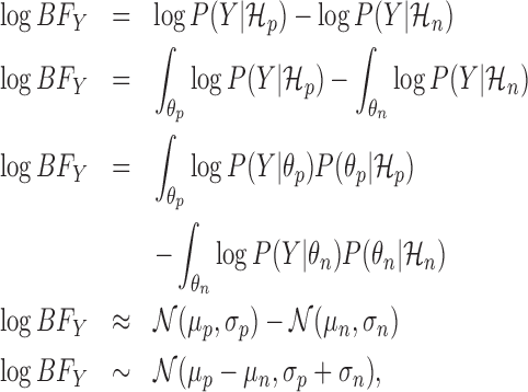
We adopt a fully Bayesian approach to calculating the Bayes factor. This allows us to propagate the uncertainty in inference encountered throughout the analysis. Rather than approximating the marginal likelihoods with point estimates, we integrate over the model parameters, as follows:

(3)

where θ_p and θ_n are the parameters of and , respectively.

In general, the integrals in Equation 3 are intractable. We use the state-of-the-art Hamiltoniam Markov chain Monte Carlo (MCMC) sampler Stan (http://mc-stan.org/) to approximate them. Stan uses the No-U Turn Sampler (NUTS) (20) to effectively tune the MCMC parameters. Long runs of the sampler are guaranteed to converge to the true distribution (21).

In practice, We selected 200 iterations of MCMC as a reasonable tradeoff between computational cost and convergence. The first 100 iterations are treated as burn-in and discarded; we fit a normal distribution for the likelihood of each model based on the final 100 iterations and approximate P(Y| · ) by the mean and variance of this distribution.

After estimating the Bayes’ factor for metagene profile Y, we select when P(log BF_Y > 5) > k, where k is a constant between 0 and 1. We use k = 0.5. This approach explicitly incorporates the uncertainty of inference because of the final probability calculation.

We construct the filtered genome profile from the base genome profile in two steps. First, reads of lengths for which was not selected are removed. Second, the remaining reads are shifted according to the calculated P-site offset for their respective lengths.

ORF extraction and profile construction

We extract ORFs based on transcript exon structures. They could come from standard annotations or de novo transcript assembly from RNA-seq, or both. In particular, we first extract the spliced transcript sequences of all isoforms. We then define an ORF as a start codon until the next in-frame stop codon. (In this work, we consider AUG as the only start codon; the software allows the user to specify other sequences as start codons.) This definition allows multiple start codons to use the same stop codon, but each start codon will only match a single stop codon. Finally, we extract the profile of the ORF by splicing the relevant portions of the filtered genome profile. Thus, the profile Y for ORF o can be considered as , where gives the number of 5΄ ends which map to position i in the ORF, after filtering and shifting reads due to the P-site offsets, and n is the length of the ORF.

Combining replicates

We use a simple approach to incorporate replicates in Rp-Bp. In particular, we create the ORF profiles as described above for each replicate. We then construct the combined ORF profile by summing the profiles from all replicates: , where R is the number of replicates and is the profile for ORF o in replicate r.

While this approach is conceptually simple, it has several important properties. First, it allows selection of different read lengths from different replicates. Furthermore, P-sites offsets for reads of the same length can differ between replicates.

Filtering unlikely ORFs

The primary assumption underpinning our approach is that the profiles of translated ORFs exhibit a clear ‘high-low-low’ pattern. Based on this, we incorporate two simple filters for the ORF profiles.

• The profile under consideration must have at least five mapped ribo-seq reads.

• The number of reads mapped to the first reading frame must exceed the number mapped in either of the other two reading frames, individually.

This filtering brings two benefits. First, it saves computations by not considering ORFs which are very unlikely to be translated. Second, as described in more detail later, the second filter simplifies our models and makes the resulting MCMC simulations easier.

Smoothing profiles

The profiles based only on ribo-seq counts tend to be very spiky and sparse. Therefore, we smooth the profiles before proceeding to the translation prediction phase. We use LOWESS (22); however, we smooth the counts from each frame separately. That is, we construct sequences Y^{o, 1}, Y^{o, 2} and Y^{o, 3}, where , where n is the length of the ORF and [m] is the set of integers {1, …, m}. We use a bandwidth parameter of 0.2 for smoothing the frame-specific profile. After smoothing, we stitch the smoothed profile back together.

Translation prediction

The goal of this work is to identify ORFs which are translated based on the (smoothed) ribo-seq profiles. We accomplish this goal by proposing a mixture model-based translation model, and an untranslated model, . After fitting each model to an ORF profile, we label it as ‘translated’ if it is better explained by , according to the Bayes factor (19). Similar approaches have been proposed in other contexts (23,24).

Translation model

The ORF translation model is conceptually similar to the metagene profile periodicity model described earlier. The translation model is essentially a mixture model which comprises one state for in-frame positions and a second for the other two frames. It also looks for ‘high-low-low’ patterns in profiles. A ‘high’ state h accounts for the in-frame observations, while a ‘low’ statelmodels observations from the other frames. For an observed ORF profile Y, the observation model is as follows:

(4)

where y_i gives the profile value at position i. The hyperparameters are again empirical estimates from the data. The full model is given in the Supplementary Data.

As previously described, we filter all ORFs for which the number of reads in the second or third reading frames exceed that of the first reading frame. Thus, we do not constrain the mean values of the model components, μ_h and μ_l. Because of this filtering, they remain semantically correct.

Background model

We use a Gaussian naïve Bayes model to recognize untranslated ORFs. It uses Equation 2 as its observation model. We refer to the model as .

Bayesian model selection and inference

We use exactly the same model selection and inference techniques described previously to select between and . Again, we explicitly incorporate the uncertainty in inference while making predictions. The experimental results confirm that this methodology leads to high-quality predictions.

Final prediction set

As described above, multiple ORFs may use the same stop codon. For downstream analysis, we select the longest ORF predicted as translated for each stop codon. Finally, among each group of overlapping ORFs, we select the one with the highest expected Bayes factor.

We label the selected ORFs according to their position and exon structure. We use the following labels: canonical, can. variant (canonical variants, such as truncations), uORF (upstream ORFs), dORF (downstream ORFs), ncRNA and other. Additionally, we have novel ORFs which come only from a de novo assembly for Caenorhabditis elegans. The Supplementary Data precisely defines these labels.

RESULTS

In this section, we evaluate Rp-Bp on several ribo-seq datasets using both standard annotations and de novo transcript assemblies, described shortly. First, we examine the basic characteristics of the predictions, like the types of ORFs. Experiments demonstrate that the Bayesian length selection technique leads to more canonical and fewer out-of-frame predicted ORFs; we then confirm that the predictions are of high quality with proteomics data and a complementary sequencing technique, QTI-seq. This validation also includes comparison to RiboTaper (16), another recently-proposed approach for identifying translation from ribo-seq data.

Throughout our analysis, we distinguish between micropeptides and longer ORFs. We call any ORF with length <300 nt as a micropeptide. Micropeptides have been repeatedly discussed as potent functional entities in the literature (e.g. ref. (25)).

Our analysis includes datasets from human, mouse and C. elegans. Furthermore, the human datasets come from cell cultures, the mouse datasets are tissue-specific and the C. elegans datasets are whole-body. Additionally, we analyze the human and mouse datasets in isolation; the C. elegans datasets include replicates. Thus, we demonstrate that Rp-Bp is widely applicable to diverse species and biological experimental designs.

Datasets

In this analysis, we use ten ribo-seq datasets (Table 1): two HEK293 samples and two mouse samples from previous publications, and six unpublished samples from C. elegans. Sample preparation and sequencing protocols for the C. elegans samples are given in the Supplementary Data. As Table 2 shows, the quality of the datasets varies substantially. For example, the protocol used to create HEK293 included an rRNA depletion step, so it includes very few reads which map to ribosomal sequences. On the other hand, for example, pre-processing leaves only about 1 000 000 reads for analysis of the M. Liver and C. elegans datasets.

Table 1. The names, abbreviations, original publications and Short Read Archive run accessions of the datasets used in this analysis.

Dataset	Abbreviation	Source	SRR accession
Human HEK293 cells	HEK293	(16)	SRR2433794
Human HEK293 cells	HEK293-Gao	(18)	SRR1630831
Mouse liver cells	M. Liver	(18)	SRR1630812
Mouse endoplasmic fibroblasts	M. EF	(18)	SRR1630816
C. elegans, Dauer 0 h	0 h	unpublished	SRR5026356
C. elegans, Dauer-exit 0.5 h	0.5 h	unpublished	SRR5026359
C. elegans, Dauer-exit 1 h	1 h	unpublished	SRR5026589
C. elegans, Dauer-exit 2 h	2 h	unpublished	SRR5026592
C. elegans, Dauer-exit 3 h	3 h	unpublished	SRR5026603
C. elegans, Dauer-exit 4 h	4 h	unpublished	SRR5026637
C. elegans (aggregate)	C. elegans	unpublished

Table 2. The number and percent of reads filtered at each stage of pre-processing for all datasets used in this section.

	M. Liver	M. EF	HEK293	HEK293, Gao	C. elegans (aggregate)
Raw data	9E + 6	3E + 7	3E + 7	3E + 7	9E + 8
Poor quality	8E + 4 (1%)	4E + 5 (1%)	5E + 5 (2%)	3E + 5 (1%)	4E + 7 (4%)
Ribosomal	5E + 6 (55%)	6E + 6 (17%)	2E + 6 (7%)	2E + 7 (66%)	5E + 8 (56%)
No alignment	1E + 6 (15%)	9E + 6 (27%)	3E + 6 (11%)	3E + 6 (10%)	2E + 8 (25%)
Multimappers	6E + 5 (7%)	8E + 6 (23%)	6E + 6 (20%)	2E + 6 (9%)	3E + 7 (3%)
Non-periodic	1E + 5 (1%)	4E + 5 (1%)	4E + 5 (2%)	1E + 5 (0%)	6E + 7 (7%)
Usable	1E + 6 (21%)	1E + 7 (31%)	1E + 7 (59%)	4E + 6 (14%)	4E + 7 (5%)

‘Raw data’ gives the total number of reads in the dataset. ‘Poor quality’ reads are either too short after removing adapters or do not have adequate fastq quality scores. ‘Ribosomal’ reads map to known ribosomal sequences. ‘No alignment’ reads do not align to the genome. ‘Multimappers’ map to the genome in multiple locations. ‘Non-periodic’ reads are of lengths whose metagene profiles do not result in a periodic signal. ‘Usable’ reads are kept for further analysis. The detailed counts for all samples, including all C. elegans replicates, are given in Supplementary File 7. We obtain a much higher percentage of rRNA reads from dauer stage lysates than from lysates of other developmental stages of the C. elegans life cycle (2).

We did not treat any of the HEK293 or mouse datasets as replicates. Therefore, the replicate-combining technique in the ‘Materials and Methods’ section was not used in their analysis.

The six C. elegans ribo-seq libraries capture the first 4 h of the dauer exit program in C. elegans. We maximize our detection sensitivity by using them as replicates in translation detection as described in the ‘Materials and Methods’ section.

We use the hg19 genome reference, GENCODE version 19 annotations and NCBI reference sequence NR_046235.1 as the ribosomal sequence for the human data. For the mouse data, we use the GRCm38 genome reference and EnsEMBL 79 annotations; the ribosomal sequence for mouse is GenBank sequence BK000964.3.

For our C. elegans analysis, we use the WBcel235 genome reference and corresponding EnsEMBL 79 annotations. Furthermore, we augment transcript models by assembling newly generated mRNA-seq datasets, which were generated from dauer larvae at the onset of dauer exit and after 8 h of dauer exit. The de novo assembly is available in Supplementary File 1.

We merge the WBcel235 annotations with those from our reference-guided de novo assembly. We label any ORF which falls entirely on a transcript from the de novo assembly as novel. We use GenBank sequence X03680.1 to filter for C. elegans ribosomal sequences.

All information on the final predicted ORFs for all datasets are available as Supplementary Files 2–6.

Predicted ORF characteristics

Translated ORF types

Table 3 shows that the proportions of ORF types predicted by Rp-Bp for the human and mouse datasets are similar. Around 75% of the predicted ORFs are canonical, annotated coding regions or variants, while about 20% of the translated ORFs come from annotated 5΄ leaders or non-coding regions; the remaining translated ORFs are located in either annotated 3΄ trailers or are out-of-frame with respect to the annotated coding regions. These results are consistent with other ribosome profiling studies (14,16).

Table 3. The number of ORFs of each type predicted by Rp-Bp.

	C. elegans	HEK293	HEK293, Gao	M. EF	M. Liver
canonical	11 558 (82%)	11 056 (64%)	8237 (60%)	9471 (59%)	549 (65%)
can. variant	1918 (14%)	1097 (6%)	2129 (16%)	1187 (7%)	1918 (22%)
uORF	71 (1%)	2244 (13%)	1216 (9%)	1858 (12%)	456 (5%)
dORF	35 (0%)	383 (2%)	425 (3%)	1719 (11%)	45 (1%)
ncRNA	254 (2%)	2 201 (13%)	1115 (8%)	1355 (8%)	154 (2%)
other	154 (1%)	217 (1%)	554 (4%)	490 (3%)	453 (5%)
novel	41 (0%)

The ORF types are described in the Supplementary Data.

We see a different story for C. elegans, though. Almost all of the Rp-Bp ORFs are canonical or canonical variants. Indeed, there are very few uORFs or dORFs predicted as translated. We attribute these differences to the fundamental different genome organization and annotation quality of C. elegans.

In the Supplementary Data, we show the metagene profiles of the translated ORF types. As previously observed (14), a spike is present in reads mapping to both the start and stop codons for all ORF types for almost all samples; the M. Liver and C. elegans datasets do not exhibit a spike at the stop codons, though. These results confirm that Rp-Bp identifies ORFs with the hallmarks of translation.

UniRef comparison

As a final validation of the basic characteristics of the predicted ORFs, we compared their lengths to the lengths of proteins in the UniRef90 database (26). We also included ORF predicted as translated by RiboTaper. Supplementary Figure S3 shows that the lengths of Rp-Bp ORFs match those in UniRef90 much better than those predicted by RiboTaper. In general, UniRef90 includes more short ORFs (not including micropeptides, ORFs with length <300 bp) than identified by either method; however, the number of longer Rp-Bp ORFs is similar to the number present in UniRef90, while RiboTaper predicts many more longer ORFs.

The length distribution of the Rp-Bp ORFs for C. elegans closely follows that of C. elegansUniRef90. Since so many of the predicted ORFs are canonical, this is unsurprising.

Bayesian periodic fragment length and P-site offset selection (BPPS)

The BPPS technique has several goals. First, the approach aims to automatically select periodic read lengths in an unbiased manner, while still avoiding noisy read lengths. Second, the approach identifies non-standard (12 bp) P-site offsets. Very recent findings highlight the importance of both aspects (27). This helps to improve sensitivity in translation predictions by using more of the available reads.

To verify the efficacy of this approach, we compared the Rp-Bp ORFs found using BPPS to using standard length selection approaches. In particular, for the HEK293 dataset, we compared BPPS with using lengths 26, 28 and 29 bp and P-site offsets 9, 12 and 12 bp, respectively; for HEK293-Gao, we compare to lengths 26, 27, 28 and 29 bp and P-site offsets of 12 bp for all lengths. These lengths and offsets were manually selected and used in previous analysis (16).

Similarly, previous analysis (18) of M. EF and M. Liver used all reads of lengths 25–35 and P-site offsets of 12 bp for all read lengths; we compare our Bayesian length selection approach to those values. In the Supplementary Data, we examine the differences among the C. elegans replicates.

Differences in BPPS and manual selections

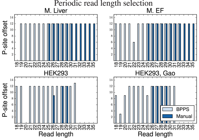
First, Figure 3 confirms that BPPS identifies many more periodic read lengths than the restricted manual selection for HEK293 and HEK293-Gao. The main disagreement between the automatic selection and manual curation is the P-site offset for reads of length 26 bp in HEK293; however, using an offset of either 9 or 12 bp does not result in a change of frame for those reads. BPPS does remove some non-periodic read lengths from downstream analysis, such as reads of length 20 bp for HEK293. Additionally, the automatic approach does identify non-standard P-site offsets, such as 13 bp for HEK293 reads of length 31 and 3 bp for HEK293-Gao reads of length 19 bp.

Figure 3.

The selected read lengths and P-site offsets selected by BPPS compared to manual selection.

On the other hand, when compared to the very broad selections originally made for M. EF and M. Liver, our approach does not include the longer reads. Instead, we select many of the smaller read lengths, sometimes with non-standard offsets. This highlights that manual selection may ignore useful reads while including noisy ones.

In the Supplementary Data, we further examine the differences among predictions with BPPS and manual selection based on whether the ORFs had external validation, such as proteomics. We again find no significant differences.

Differences in ORF predictions

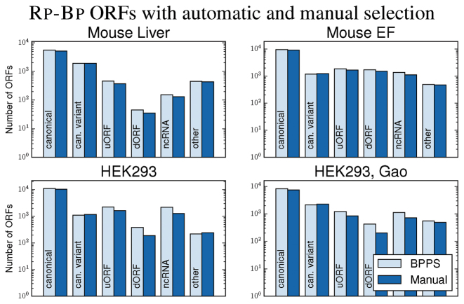
We then compared the Rp-Bp ORFs using either BPPS or manually-selected read lengths and P-site offsets. As shown in Figure 4, the different selection techniques result in modest, but distinctly different, patterns among the Rp-Bp ORFs. In particular, in both HEK293 and M. EF, BPPS results in more canonical, uORF, dORF and ncRNA ORFs, while manual selection results in more can. variant features. Both techniques result in a similar number of out-of-frame overlapping ORFs. This shows that the predictions using BPPS are of higher quality than those from manual selection. Of course, BPPS also has the advantage that it automatically adapts to choose the best lengths and offsets rather than requiring manual selection.

Figure 4.

The number of Rp-Bp ORFs using BPPS and manual length and P-site offset selection for the human and mouse datasets. The ORF types are described in the Supplementary Data.

Proteomics analysis

We next used two high-quality mass spectrometry proteomics datasets (PRIDE accessions [PXD002389 and PXD001468] and MaxQuant (28–30)) to compare the proteomics-verified support of predicted ORFs for HEK293. We compare the ORFs predicted by Rp-Bp and RiboTaper as well as those annotated as protein coding in GENCODE. We also generated a C. elegans mass spectrometry proteomics dataset to verify the predictions made by Rp-Bp; the WBcel235 annotations are used as a baseline for comparison. The details of the proteomics analysis are in the Supplementary Data.

In silico digestion

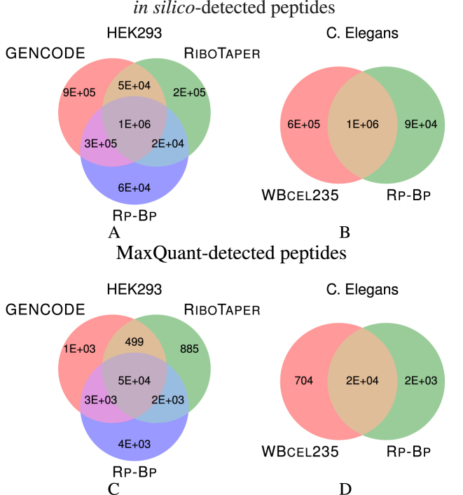
As a baseline, we first compared the theoretical number of peptide sequences each set of ORFs could possibly identify; we found these via in silico digestion of the respective peptide sequences. (More details are presented as part of the Supplementary Data.) Figure 5 shows that Rp-Bp and RiboTaper result in a similar number of peptides, while, GENCODE includes many more possible peptides. This is expected since the GENCODE annotations are not cell type-specific. According to the theoretical digestion, both Rp-Bp and RiboTaper identify tens of thousands of peptides distinct from each other and GENCODE. The differences from GENCODE arise from ncRNA and other non-canonical ORFs.

Figure 5.

The number of peptide sequences identified with (A) in silico digestion of the annotated proteins from GENCODE, and the ORFs predicted by Rp-Bp and RiboTaper for HEK293, (B) in silico digestion of the annotated proteins from WBcel235 and Rp-Bp for Caenorhabditis elegans, (C and D) MaxQuant for the respective datasets. The in silico digestion and MaxQuant details are given in the Supplementary Data.

The relative overlap among the Rp-Bp ORFs for C. elegans and the annotations is somewhat higher. As mentioned, though, many of the C. elegansRp-Bp ORFs are canonical, so it is expected that the predicted ORFs have more in common with the annotated proteins.

MaxQuant detection

We then compared the number of peptide sequences actually detected using MaxQuant for each set of ORFs. While the overlap among the three sets of ORFs from HEK293 shown in Figure 5 is quite high, Rp-Bp results in several thousand uniquely-identified peptides compared to either RiboTaper or GENCODE. In contrast, RiboTaper and GENCODE only produce about a thousand unique ORFs each. The in silico peptide analysis showed that Rp-Bp and RiboTaper yield a similar number of possible peptides, so Rp-Bp does not result in more unique peptides than RiboTaper simply because more are possible. Besides the peptides unique to Rp-Bp, another reason more peptides are detected using Rp-Bp ORFs is that it produces a smaller number of sequences than RiboTaper and GENCODE; consequently, the false discovery rate and error probabilities calculated by MaxQuant are lower. Similarly, more C. elegans peptides are detected using the Rp-Bp ORFs than annotations.

Peptide support for Rp-Bp ORF types

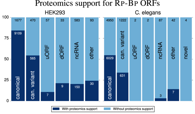
We next analyzed the peptide support for all ORFs predicted as translated by Rp-Bp. Over 75% of the canonicalRp-Bp ORFs have peptide support (Figure 6), and a majority of the canonical variants also have peptide support. Additionally, over 20% of the ORFs annotated as ncRNA or dORF, but predicted as translated, have peptide support. While the peptide support for uORFs is not as strong, in total, the proteomics analysis validates the accuracy of many of the predictions made by Rp-Bp for longer ORFs.

Figure 6.

The percentage of each type of Rp-Bp ORF (≥300 nt) from the HEK293 and Caenorhabditis elegans datasets with proteomics support. An ORF is considered to have proteomics support if at least one peptide detected by MaxQuant exactly aligns to the translated protein sequence for the ORF. Furthermore, we require the peptide uniquely align to that ORF. The numbers on the bars show the number of ORFs with and without proteomics support, as indicated.

For C. elegans, about half of the canonical ORFs, and a third of their variants, were supported by the proteomics data. However, the other ORF types do not have as much proteomics support. Nevertheless, as shown in Table 3, about 95% of the Rp-Bp ORFs arecanonical or variants. So many of the predictions do in fact have peptide support.

Comparison of Rp-Bp and RiboTaper peptide support

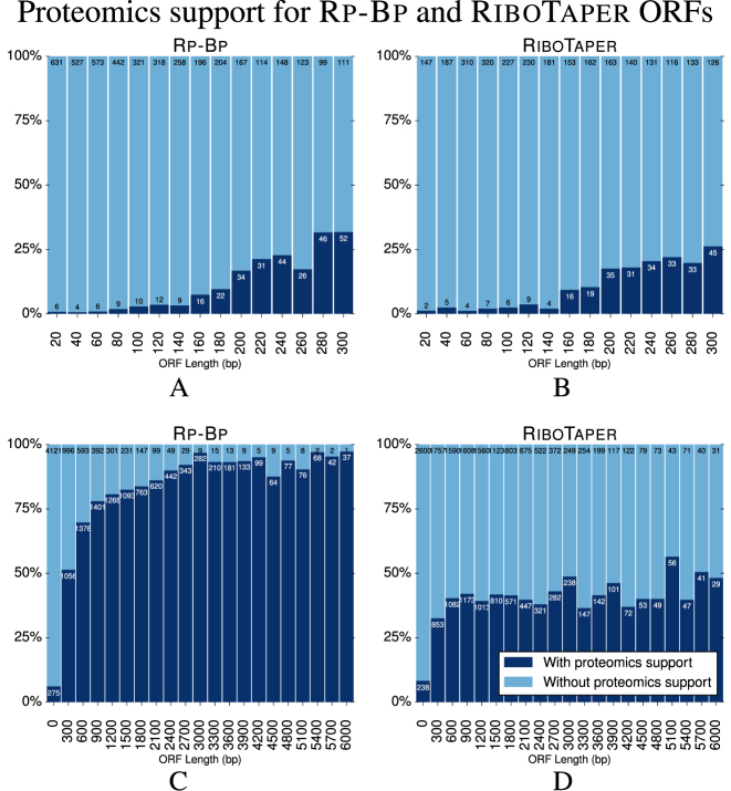
We also evaluated the peptide support of the predicted ORFs in HEK293 as a function of the length of the ORFs, shown in Figure 7. We included the ORFs predicted by RiboTaper in this evaluation. For this analysis, we again use only peptides which uniquely map to an ORF. We first considered the support of the micropeptides (ORF length <100aa). As Figure 7A and B shows, micropeptides do not have much support from the proteomics data. It is technically challenging to obtain peptide evidence from these very short proteins during the proteomics experiments and thus expected that few of these have peptide support. Still, in terms of raw numbers and percentage of predictions, more Rp-Bp micropeptides have unique proteomics support than those from RiboTaper. The Rp-Bp results for C. elegans are similar to those for HEK293.

Figure 7.

(A and B) The percentage of Rp-Bp and RiboTaper micropeptides of different lengths (<100aa) with proteomics support in HEK293. Proteomics support is described in the caption of Figure 6. All ORF types are grouped based on bin sizes of 20 bp. The numbers on the bars show the number of micropeptides with and without proteomics support, as indicated. (C and D) The percentage of all Rp-Bp and RiboTaper ORFs with unique proteomics support in HEK293. All ORF types are grouped based on bin sizes of 300 bp. The counts are also available in Supplementary File 8.

We then considered unique peptide support for longer ORFs in Figure 7C and D. Herein, the percentage of ORFs at almost all read lengths with unique peptide support is much higher for Rp-Bp on HEK293 compared to RiboTaper. As with the micropeptides, in terms of raw counts, Rp-Bp results in modestly more ORFs with unique peptide support; as discussed previously, RiboTaper predicts many more longer ORFs are translated than Rp-Bp. These results show that many of the longer ORFs do not have unique peptide support.

C. elegans micropeptides

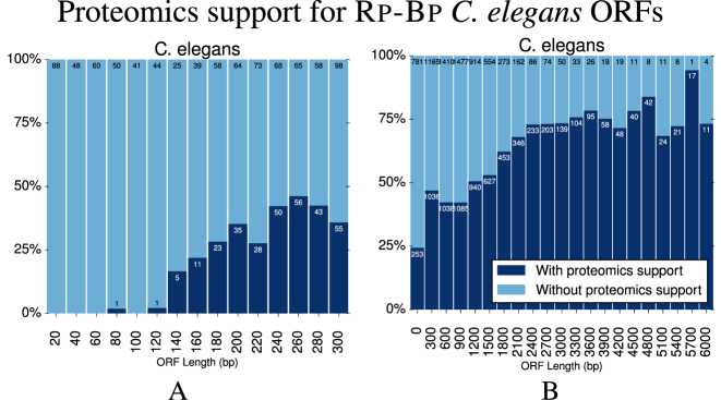
The percentage of Rp-BpC. elegans ORFs predictions, shown in Figure 8B, with unique peptide support is somewhat less than that for the human data; however, proteomics replicates were available for human, so it is unsurprising that more ORFs had proteomics validation. Nevertheless, the percentage of Rp-BpC. elegans micropeptides with proteomics validation, in Figure 8A, is somewhat higher than for the HEK293 dataset, especially for micropeptides between 150 and 300 nt.

Figure 8.

The percentage of Rp-Bp Caenorhabditis elegans (A) micropeptides and (B) all ORFs with unique proteomics support, as described in Figure 7. The counts are also available in Supplementary Table S8.

Finally, we identified 3622 novel transcripts in C. elegans with a reference-guided transcriptome assembly approach (see Supplementary File 1). Several of them harbor small ORFs that could encode for novel micropeptides in C. elegans. We predicted 41 novel ORFs as being translated, 37 of which are micropeptides (<300 bp). We found unique proteomics support for one of the micropeptides. In essence, Rp-Bp is able to identify novel coding regions even in genomes, which are excessively curated such as C. elegans.

Taken together, these results show that Rp-Bp predictions from different species are well-supported by proteomics data. The predictions result in more unique peptide identifications from proteomics data compared to standard annotations and RiboTaper predictions; a large majority of the longer ORFs have peptide support, and even many of the predicted micropeptides have support from the proteomics data.

QTI-seq analysis

QTI-seq (18) is a recently-developed protocol for identifying ribosomes initiating translation. Briefly the method consists of lysing cells, freezing initiating ribosomes with lactimidomycin and depleting elongating ribosomes with puromycin. Thus, only initiating ribosomes remain and, after further detailed protocols, the associated cDNA can be sequenced.

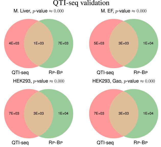
Matching QTI-seq datasets are available (18) for all human and mouse ribo-seq datasets used in this study. We matched reported QTI-seq peaks to the start codon of all annotated transcripts and compared this to the set of transcripts with Rp-Bp ORFs. The ORFs identified by Rp-Bp show very good agreement with QTI-seq peaks; as Figure 9 shows the P-values of the overlaps for all datasets are very close to 0. This gives another form of validation that the predictions by Rp-Bp accurately reflect the biology in the cell.

Figure 9.

The overlap of transcripts with a QTI-seq peak within 50 bp of the annotated start codon and a Rp-Bp ORF (of any type). The P-values are calculated using a hypergeometric test.

DISCUSSION

The ribosome profiling protocols offer a genome-wide view of the activity of the ribosome. However due to biological and technical artifacts, principled analysis techniques are required to fully leverage the ribo-seq profiles. We proposed a fully Bayesian translation prediction approach, Rp-Bp. The heart of Rp-Bp lies in state-of-the-art MCMC sampling via Stan (http://mc-stan.org/) to estimate posterior distributions from biologically-inspired models of (un)translation. Bayesian model selection is then used to estimate a posterior distribution of translation. Unlike previous work (23,24), we do not resort to point estimates, but instead maintain distributions over quantities of interest through the entire process. Thus, our pipeline propagates uncertainty to improve later predictions.

Additionally, we use the Bayesian model selection technique in a novel approach for selecting periodic ribo-seq read lengths appropriate for downstream analysis; it also automatically determines the P-site offset for each read length.

On publicly-available ribo-seq datasets, we show that the Bayesian read length selection approach results in more canonical and non-canonical ORFs predicted as translated. Furthermore, validation with high-quality proteomics and QTI-seq data confirm the predictions are of very high quality. Our proteomics analysis also demonstrates that more Rp-Bp ORFs have unique peptide alignments compared with RiboTaper (16), another recent translation-prediction pipeline. Additionally, Rp-Bp results in more peptide identifications than RiboTaper.

As suggested in the method description, one limitation of Rp-Bp is its unnormalized parameter estimates. For example, it would not be appropriate to compare estimates from two different datasets. A natural next step is normalization of the ribo-seq profiles so the parameter estimates are useful for differential translation analysis. Another venue for further development are more sophisticated models that could aid in distinguishing isoforms, detecting overlapping ORFs and identifying programed frameshifts.

AVAILABILITY

Our implementation of Rp-Bp is available at https://github.com/dieterich-lab/rp-bp. The pipeline is implemented as a set of Python3 scripts and is installed via pip. A simple driver script runs the entire pipeline; it can optionally submit the processing to the Simple Linux Utility for Resource Management (Slurm) workload manager. The software requires a genome reference fasta file and matching GTF3/GFF annotations. The final output is a valid BED12 file with the predicted ORFs, as well as DNA and protein fasta files containing the predicted sequences.

SUPPLEMENTARY DATA

Supplementary Data are available at NAR Online.

FUNDING

CD and BM were supported by the Klaus Tschira Stiftung GmbH [00.219b.2013]. The experimental work performed in H.G.'s lab was partly supported by the Swiss National Science Foundation through the NCCR RNA & Disease, and the European Union Seventh Framework Programme (FP7/2007-2013) under grant agreement no. 241985 (European Research Council “miRTurn”) (to H.G.). Funding for open access charge: Klaus Tschira Stiftung [00.219b.2013].

Conflict of interest statement. None declared.

REFERENCES

- 1. Ingolia N.T. Ribosome profiling: new views of translation, from single codons to genome scale. Nat. Rev. Genet. 2014; 15:205–213. [DOI] [PubMed] [Google Scholar]
- 2. Aeschimann F., Xiong J., Arnold A., Dieterich C., Großhans H.. Transcriptome-wide measurement of ribosomal occupancy by ribosome profiling. Methods. 2015; 85:75–89. [DOI] [PubMed] [Google Scholar]
- 3. Guttman M., Russell P., Ingolia N., Weissman J., Lander E.. Ribosome profiling provides evidence that large noncoding RNAs do not encode proteins. Cell. 2013; 154:240–251. [DOI] [PMC free article] [PubMed] [Google Scholar]
- 4. Ingolia N.T., Ghaemmaghami S., Newman J. R.S., Weissman J.S.. Genome-wide analysis in vivo of translation with nucleotideresolution using ribosome profiling. Science. 2009; 324:218–223. [DOI] [PMC free article] [PubMed] [Google Scholar]
- 5. Olshen A.B., Hsieh A.C., Stumpf C.R., Olshen R.A., Ruggero D., Taylor B.S.. Assessing gene-level translational control from ribosome profiling. Bioinformatics. 2013; 29:2995–3002. [DOI] [PMC free article] [PubMed] [Google Scholar]
- 6. Zhong Y., Karaletsos T., Drewe P., Sreedharan V., Kuo D., Singh K., Wendel H.-G., Rätsch G.. RiboDiff: detecting changes of mRNA translation efficiency from ribosome footprints. Bioinformatics. 2017; 33:139–141. [DOI] [PMC free article] [PubMed] [Google Scholar]
- 7. Gritsenko A.A., Hulsman M., Reinders M.J.T., de Ridder D.. Unbiased quantitative models of protein translation derived from ribosome profiling data. PLoS Comput. Biol. 2015; 11:e1004336. [DOI] [PMC free article] [PubMed] [Google Scholar]
- 8. Dana A., Tuller T.. The effect of tRNA levels on decoding times of mRNA codons. Nucleic Acids Res. 2014; 42:9171–9181. [DOI] [PMC free article] [PubMed] [Google Scholar]
- 9. Hussmann J.A., Patchett S., Johnson A., Sawyer S., Press W.H.. Understanding biases in ribosome profiling experiments reveals signatures of translation dynamics in yeast. PLoS Genetic. 2015; 11:e1005732. [DOI] [PMC free article] [PubMed] [Google Scholar]
- 10. Diament A., Tuller T.. Estimation of ribosome profiling performance and reproducibility at various levels of resolution. Biol. Direct. 2016; 11:24. [DOI] [PMC free article] [PubMed] [Google Scholar]
- 11. Menschaert G., Van Criekinge W., Notelaers T., Koch A., Crappé J., Gevaert K., Van Damme P.. Deep proteome coverage based on ribosome profiling aids mass spectrometry-based protein and peptide discovery and provides evidence of alternative translation products and near-cognate translation initiation events. Mol. Cell. Proteomics. 2013; 12:1780–1790. [DOI] [PMC free article] [PubMed] [Google Scholar]
- 12. Crappé J., Ndah E., Koch A., Steyaert S., Gawron D., De Keulenaer S., De Meester E., De Meyer T., Van Criekinge W., Van Damme P. et al. PROTEOFORMER: deep proteome coverage through ribosome profiling and MS integration. Nucleic Acids Res. 2015; 43:e29. [DOI] [PMC free article] [PubMed] [Google Scholar]
- 13. Bazzini A.A., Johnstone T.G., Christiano R., Mackowiak S.D., Obermayer B., Fleming E.S., Vejnar C.E., Lee M.T., Rajewsky N., Walther T.C. et al. Identification of small ORFs in vertebrates using ribosome footprinting and evolutionary conservation. EMBO J. 2014; 33:981–993. [DOI] [PMC free article] [PubMed] [Google Scholar]
- 14. Fields A.P., Rodriguez E.H., Jovanovic M., Stern-Ginossar N., Haas B.J., Mertins P., Raychowdhury R., Hacohen N., Carr S.A., Ingolia N.T. et al. A regression-based analysis of ribosome-profiling data reveals a conserved complexity to mammalian translation. Mol. Cell. 2015; 60:816–827. [DOI] [PMC free article] [PubMed] [Google Scholar]
- 15. Raj A., Wang S.H., Shim H., Harpak A., Li Y.I., Engelmann B., Stephens M., Gilad Y., Pritchard J.K.. Thousands of novel translated open reading frames in humans inferred by ribosome footprint profiling. Elife. 2016; 5:e13328. [DOI] [PMC free article] [PubMed] [Google Scholar]
- 16. Calviello L., Mukherjee N., Wyler E., Zauber H., Hirsekorn A., Selbach M., Landthaler M., Obermayer B., Ohler U.. Detecting actively translated open reading frames in ribosome profiling data. Nat. Methods. 2015; 13:165–170. [DOI] [PubMed] [Google Scholar]
- 17. Popa A., Lebrigand K., Paquet A., Nottet N., Robbe-Sermesant K., Waldmann R., Barbry P.. RiboProfiling: a Bioconductor package for standard Ribo-seq pipeline processing [version 1; referees: 3 approved]. F1000 Res. 2016; 5:1309. [DOI] [PMC free article] [PubMed] [Google Scholar]
- 18. Gao X., Wan J., Liu B., Ma M., Shen B., Qian S.-B.. Quantitative profiling of initiating ribosomes in vivo. Nat. Methods. 2015; 12:147–153. [DOI] [PMC free article] [PubMed] [Google Scholar]
- 19. Kass R.E., Raftery A.E.. Bayes Factors. J. Am. Stat. Assoc. 1995; 90:773–795. [Google Scholar]
- 20. Hoffman M.D., Gelman A.. The No-U-Turn sampler: adaptively setting path lengths in Hamiltonian Monte Carlo. J. Mach. Learn. Res. 2014; 15:1593–1623. [Google Scholar]
- 21. Brooks S.P., Gelman A.. General methods for monitoring convergence of iterative simulations. J. Comput. Graph. Stat. 1998; 7:434–455. [Google Scholar]
- 22. Cleveland W.S. Robust locally weighted regression and smoothing scatterplots. J. Am. Stat. Assoc. 1979; 74:829–836. [Google Scholar]
- 23. Kalaitzis A., Lawrence N.. A simple approach to ranking differentially expressed gene expression time courses through Gaussian process regression. BMC Bioinformatics. 2011; 12:180. [DOI] [PMC free article] [PubMed] [Google Scholar]
- 24. Topa H., Jonas A., Kofler R., Kosiol C., Honkela A.. Gaussian process test for high-throughput sequencing time series: application to experimental evolution. Bioinformatics. 2015; 31:1762–1770. [DOI] [PMC free article] [PubMed] [Google Scholar]
- 25. Payre F., Desplan C.. Small peptides control heart activity. Science. 2016; 351:226–227. [DOI] [PMC free article] [PubMed] [Google Scholar]
- 26. Suzek B.E., Huang H., McGarvey P., Mazumder R., Wu C.H.. UniRef: comprehensive and non-redundant UniProt reference clusters. Bioinformatics. 2007; 23:1282–1288. [DOI] [PubMed] [Google Scholar]
- 27. Baranov P.V., Loughran G.. Catch me if you can: trapping scanning ribosomes in their footsteps. Nat. Struct. Mol. Biol. 2016; 23:703–704. [DOI] [PubMed] [Google Scholar]
- 28. Eravci M., Sommer C., Selbach M.. IPG Strip-based peptide fractionation for shotgun proteomics. Methods Mol. Biol. 2014; 1156:67–77. [DOI] [PubMed] [Google Scholar]
- 29. Chick J.M., Kolippakkam D., Nusinow D.P., Zhai B., Rad R., Huttlin E.L., Gyg S.P.. A mass-tolerant database search identifies a large proportion of unassigned spectra in shotgun proteomics as modified peptides. Nat. Biotechnol. 2015; 33:743–749. [DOI] [PMC free article] [PubMed] [Google Scholar]
- 30. Cox J., Mann M.. MaxQuant enables high peptide identification rates, individualized p.p.b.-range mass accuracies and proteome-wide protein quantification. Nat. Biotechnol. 2008; 26:1367–1372. [DOI] [PubMed] [Google Scholar]
Associated Data
This section collects any data citations, data availability statements, or supplementary materials included in this article.