Adaptive Local Window for Level Set Segmentation of CT and MRI Liver Lesions

Abstract

We propose a novel method, the adaptive local window, for improving level set segmentation technique. The window is estimated separately for each contour point, over iterations of the segmentation process, and for each individual object. Our method considers the object scale, the spatial texture, and the changes of the energy functional over iterations. Global and local statistics are considered by calculating several gray level co-occurrence matrices. We demonstrate the capabilities of the method in the domain of medical imaging for segmenting 233 images with liver lesions. To illustrate the strength of our method, those lesions were screened by either Computed Tomography or Magnetic Resonance Imaging. Moreover, we analyzed images using three different energy models. We compared our method to a global level set segmentation, to a local framework that uses predefined fixed-size square windows and to a local region-scalable fitting model. The results indicate that our proposed method outperforms the other methods in terms of agreement with the manual marking and dependence on contour initialization or the energy model used. In case of complex lesions, such as low contrast lesions, heterogeneous lesions, or lesions with a noisy background, our method shows significantly better segmentation with an improvement of 0.25 ± 0.13 in Dice similarity coefficient, compared with state of the art fixed-size local windows (Wilcoxon, p < 0.001).

Graphical abstract

1. Introduction

Liver lesion segmentation is a well-studied area that has several applications, such as treatment assessment, and computer-assisted diagnosis. Manual segmentation of lesions is time-consuming, tedious procedure, which is highly depended on the user experience (Hame and Pollari, 2012). Therefore, many works in literature suggest accurate and robust automatic liver lesion segmentations. Shimizu et al. (2008) used the AdaBoost technique to segment liver lesions based on local image features. Pescia et al. (2008) also uses texture features to segment liver lesions. The method of Moltz et al. (2009), which combines a threshold-based approach with model-based morphological operations, can segment 3D liver lesions with 31% error. Abdel-Massieh et al. (2010) incorporates intensity and shape information while Militzer et al. (2010) utilizes a probabilistic boosting tree for lesion segmentation. Masuda et al. (2010) proposed a method that classifies voxels into normal and abnormal tissues using expectation–maximization and uses a morphological filter that incorporates circularity and proximity to boundary to eliminate false positives. The method of Wu et al. (2012) combines gradient-based locally adaptive segmentation with intensity and geometric features-based classification. Schwier et al. (2011) and Yan et al. (2015) apply watershed transformation for segmentation of liver lesions. Cao et al. (2016) presents a technique for segmenting lesions according to their intensity and location properties, based on Iterative Relative Fuzzy Connectedness method; however, it has difficulties in handling heterogeneous liver lesions. Additional recent work on liver and lesion segmentation employs sigmoid edge modeling (Foruzan and Chen, 2015) or machine learning techniques (Freiman et al., 2011; Kadoury et al., 2015). Other works apply graph cut techniques (Li et al., 2015; Linguraru et al., 2012).

Level set techniques are another popular approach that is used for liver lesion segmentation due to their ability to handle image noise, intensity heterogeneities, and discontinuous object boundaries (Casciaro et al., 2012; Li et al., 2013; Li et al., 2011). The semi-automatic method presented by Smeets et al. (2010) is based on a level set fitted on a fuzzy classification of the image data. The contour initialization is generated by a spiral-scanning technique based on dynamic programming. The method performed well in the 3D Liver Tumor Segmentation Challenge 2008 (Deng and Du, 2008), but its performance is limited in low contrast lesions. In addition, it does not perform well when lesions that are surrounded by other pathologic tissues.

Level set methods include both edge-based (Caselles et al., 1997; Li et al., 2005; Malladi et al., 1995; Osher and Sethian, 1988) and region-based models (Chan and Vese, 2001; Lankton et al., 2007; Lankton and Tannenbaum, 2008; Li et al., 2007; Li et al., 2008; Mumford and Shah, 1989; Ronfard, 2002; Tsai et al., 2001; Vese and Chan, 2002;). Edge-based models are not ideal for noisy images, objects with incomplete boundaries, or objects with low object-to-background contrast. Region-based models estimate spatial statistics of image regions to find the minimal energy where the model best fits the image. Chan and Vese (2001) applied a region-based segmentation model with global constraint, based on the Mumford and Shah functional. The main advantage of the global constraint is its high robustness to the location of the initial contour (Chan and Vese, 2001; Yezzi et al., 2002). However, in many cases such as with heterogeneous intensity areas, a local framework performs better than a global one (Lankton and Tannenbaum, 2008; Li et al., 2007; Li et al., 2008; Malladi et al., 1995; Zheng et al., 2013; Zhang et al., 2010; Wang et al., 2009). Hybrid models are superior, defining an energy functional with local and global constraints to obtain a more accurate segmentation that is more robust to contour initialization (Smeets, et al., 2008; Zhang et al., 2010). Those methods allow curve deformation to find only significant local minima and delineate object borders despite noise, poor edge information, and heterogeneous intensity profiles (Lankton et al., 2007).

Robustness to initial conditions is an important measure of segmentation performance. Initial shape and position parameters (size, rotation, and location) need to be adequately determined; otherwise, the contour may converge to a local minimum and fail to capture the features of interest. The most common techniques for contour initialization are 1) manual selection of initial points (Ardon and Cohen, 2006; Cohen and Kimmel, 1997; Neuenschwander et al., 1994); 2) analysis of the external force field (Ge and Tian, 2002; He et al., 2006; Liu and Fox, 2005; Tauber et al., 2005); 3) naive geometric models such as a circle in 2-D or sphere in 3-D; and, 4) learned shape priors, where a statistical shape model is estimated, and the automated procedure then tries to find the segmentation that best fits the shape model (Cootes et al., 1999; Das et al., 2006; Freedman and Zhang, 2005; Tsai et al., 2003). However, methods based on shape priors may be restrictive in applications involving highly variable shapes.

Though the accuracy of contour initialization is important, the size of the local window surrounding each contour point plays a key role in the segmentation performance. The window size defines how the local scale of the statistics evaluation, and thus must be selected appropriately, even when initialization of the active contour is relatively accurate. Furthermore, well-defined local window can compensate on low-quality initial contour. Most local segmentation methods use candidates for pre-defined window sizes as input. Each candidate window size is tested over an extensive sequence of images to ascertain the best window size and this fixed window size is used for the entire database of images. However, this window size will not be optimal for all images and new images with different spatial statistics may require additional experiments to find the best window size. Thus, choosing a fixed window size by trial and error is a time consuming process. Moreover, when the images contain substantial diversity of spatial characteristics, pre-defining a single window size may result in non-optimal segmentation performance for all images. For that reason, a varied window size that is defined adaptively according to spatial information has a greater chance of providing accurate segmentation.

An et al. (2007) implemented a local framework at two different scales and showed that segmentation performance is better when using more than one scale. Li et al. (2008) studied in-depth the selection of kernel functions and its effect on segmentation performance. The authors applied their method using three different predefined Gaussian scales. The most accurate segmentation was obtained by using the smallest scale, but their method was more robust to contour initialization using a larger scale (Li et al., 2008), creating a trade-off when choosing a local scale. For those multi-scale methods (An et al., 2007; Li et al., 2008), a pre-specified pyramid of discrete Gaussian scales should be supplied as input. Using pre-specified scales may lead to a high dependence of segmentation accuracy on the number and the values of the discrete scales input.

Recently published research provides methods to select the best scale from a range of input scales. Yang and Boukerroui (2011) proposed a Gaussian scale selection based on the intersection of confidence intervals rule: the local scale is estimated by minimizing the mean square error of a local polynomials approximation (LPA). Pivano and Papadopoulo (2008) also applied a given pyramid of Gaussian kernels to compute local means and variances. They recommend choosing a scale that is the smallest one that induces an evolution speed greater than a user-determined threshold (Piovano and Papadopoulo, 2008). Choosing a single scale has some drawbacks. First, it may be sensitive to the criteria used. Second, since scale choice is done by examining a specific scale, it is based on the local window only; however, in many cases such as low contrast objects, heterogeneous objects or objects with a noisy background, global information can contribute substantially to segmentation performance and thus should be considered when a scale is chosen. Finally, these methods use the same chosen single scale during the whole segmentation process.

We propose a method to overcome these limitations by adaptively estimating the appropriate local window size for each contour point. The local window size is re-estimated at each point by an iterative process that considers the object scale, local and global texture statistics, and minimization of the cost function, thus generating an adaptive local window. Further, this proposed method estimates the size of the local window directly from the image, not by testing a specific scale from a range of scales and thus requires no pyramid of pre-defined scales as input, removing any potential sensitivity to user input regarding scale sizes. To the best of our knowledge, this kind of method has never been described before.

We study the effect of the adaptive window size on segmentation results in-depth, and demonstrate the capabilities and strength of our method through analysis of clinically-diagnosed lesions imaged by two different imaging modalities (CT and MRI). We use three different local energy models for image analysis of these lesions to confirm the method works with a variety of models, and compare our method to results from analyses using a global segmentation and a pre-defined fixed-size square window in local segmentation framework.

In section 2, we present the global and the local energy models that are the basis for our image analysis. Section 3 presents our method for estimating the adaptive local window. In sections 4 and 5, we discuss the key ideas regarding the implementation and the experimental data. In section 6, we present the results and compare the adaptive local window model with common-used methods. Section 7 discusses results and provides some concluding remarks.

2. Energy Models

We used three different energy models to extensively evaluate our proposed adaptive local window. The piecewise constant model provides both a global and local energy frameworks. We also use the local mean separation and histogram separation energy models.

2.1. Piecewise constant (PC) model

Chan and Vese (2001) present a global framework of the PC model, which assumes that an image I is formed by two distinct areas (object and background areas), each of which have homogeneous intensities. Let M_u and M_v represent the mean intensity of the object and its background, respectively. Set Ω as a bounded subset in R² and I(x, y) as the coordinates of a point on image I. Let ϕ(x, y) be a signed distance map and ∇ be the first variation of the energy with respect to the distance map ϕ(x, y). Let F_PC(M_u, M_v, ϕ) be a function that models the object and its background:

$$\begin{array}{l}{F}_{MS}(m_u,m_v,\varphi )=\mu \underset{{\mathrm{\Omega }}_n}{\int }\delta \varphi (x,y)\left|\nabla \varphi (x,y)\right|\mathit{dxdy}+\\ {\lambda }_1\underset{{\mathrm{\Omega }}_n}{\int }{\left|\frac{I(x,y)-m_u}{A_u}\right|}^{2}H\varphi (x,y)\mathit{dxdy}+\\ {\lambda }_2\underset{{\mathrm{\Omega }}_n}{\int }{\left|\frac{I(x,y)-m_v}{A_v}\right|}^2\left(1-H\varphi (x,y)\right)\mathit{dxdy}.\end{array}$$ (1)

where μ affects the smoothness of the curve, and Hϕ(x, y) is given by the Heaviside function as is presented in (Chan and Vese, 2001). A local version of the PC model can by used by replacing M_u and M_v with their local versions, m_u and m_v, to represent the local means of a region surrounding each contour point (Lankton and Tannenbaum, 2008).

2.2. Mean separation (MS) model

The mean separation model was first proposed by Yezzi et al. (2002). It assumes that the object and its background have maximal separation between mean intensities:

$$\begin{array}{l}{F}_{PC}(M_u,M_v,\varphi )=\mu \underset{\mathrm{\Omega }}{\int }\delta \varphi (x,y)\left|\nabla \varphi (x,y)\right|\mathit{dxdy}+\\ {\lambda }_1\underset{\mathrm{\Omega }}{\int }{\left|I(x,y)-M_u\right|}^{2}H\varphi (x,y)\mathit{dxdy}+\\ {\lambda }_2\underset{\mathrm{\Omega }}{\int }{\left|I(x,y)-M_v\right|}^2\left(1-H\varphi (x,y)\right)\mathit{dxdy},\end{array}$$ (2)

Here, Ω_n ∈ R² is the local version of Ω that represents the narrow-band points only. A_u and A_v are the areas of the local interior and exterior regions surrounding a contour point, respectively:

$$A_u=\underset{{\mathrm{\Omega }}_n}{\int }H(\varphi )(x,y)\mathit{dxdy},A_v=\underset{{\mathrm{\Omega }}_n}{\int }(1-H\varphi (x,y))\mathit{dxdy}.$$ (3)

The MS energy is minimized when |m_u − m_v| is maximized. In some cases, the MS model supplies better results than the PC model due to its use of the maximal contrast between the interior and the exterior regions without any restrictions on intensity homogeneity/uniformity within each region.

2.3. Histogram separation (HS) model

The HS model also allows for heterogeneous intensities. Let p_u(b) and p_v(b) be two intensity histograms computed from local interior and exterior regions, respectively, that surround each ZLS contour point, where N is the number of histogram bins. The Bhattacharyya coefficient B is used to evaluate the similarity of the two histograms (Bhattacharyya, 1943):

$$B=\underset{b=1}{\overset{N}{\int }}\sqrt{p_u(b)p_v(b)}db.$$ (4)

Using separate intensity histograms allows the interior and exterior regions to be heterogeneous, as long as their intensity histograms differ from each other. By using the Bhattacharyya metric to quantify the separation of the intensity histograms, we can segment objects that have local non-uniform intensities. Thus, no preliminary assumption regarding the gray level distribution of the object is made; however, the intensity profile of the entire object and the entire background must be distinct. We can then model the image using:

$$\begin{array}{l}{F}_{HS}(x,y,\varphi )=\underset{{\mathrm{\Omega }}_n}{\int }B·\left(\frac{1}{A_u}-\frac{1}{A_v}\right)\mathit{dxdy}+\\ {\lambda }_1\underset{{\mathrm{\Omega }}_n}{\int }\left(\frac{1}{A_u}\times \sqrt{\frac{p_u(x,y)}{p_v(x,y)}}H\varphi (x,y)\right)\mathit{dxdy}+\\ {\lambda }_2\underset{{\mathrm{\Omega }}_n}{\int }\left(\frac{1}{A_v}\times \sqrt{\frac{p_v(x,y)}{p_u(x,y)}}\left(1-H\varphi (x,y)\right)\right)\mathit{dxdy},\end{array}$$ (5)

3. The proposed method

The PC, MS and HS local models require that a regional window be defined in which the energy cost function can be calculated. Here, we present a method to estimate adaptively the size of the local window surrounding each contour point. The size of the local window depends on 1) lesion size, 2) spatial texture, and 3) convergence of the energy functional over iterations (Fig. 1). The process is applied iteratively for each ZLS contour point, and for each lesion separately. We expect that using different window sizes for different lesions and contour points will lead segmentation to fit better with changes in the spatial statistics (Fig. 2). To best accommodate varying spatial characteristics, the window size is estimated for the X and Y dimensions separately using the texture component of the appropriate axis only.

Fig 1.

Main steps of the proposed method. The upper scheme presents the overall segmentation procedure. The lower scheme focuses specifically on the proposed method - calculation of the local adaptive window.

Fig 2.

Adaptive local window sizes estimated for different lesions and different contour points. For each image, the adaptive local window size chosen is shown for two different contour points (a) Low contrast MRI liver lesion. Yellow window – 2.4 mm × 4 mm, green window – 4 mm × 4 mm. (b) Noisy CT liver lesion. Yellow window – 8 mm × 8 mm, green window – 7 mm × 9 mm. Red contour – radiologist manual marking. White contour – initial zero level set (ZLS) contour.

3.1. Adaptive Local Window (ALW)

The adaptive local window depends on the size of the lesion to be segmented. It should be smaller for smaller lesions. The adaptive window also depends on the spatial texture of the lesion and its background. The window should ensure convergence of the Zero Level Set (ZLS) contour towards the lesion boundaries, even in the case of low contrast lesions, while preventing convergence of the contour into local minima in cases of a noisy background. We thus estimate the appropriate local window size using also texture analysis, done by extracting Haralick texture features, i.e. contrast and homogeneity, from a second order statistics model, the gray-level co-occurrence matrices (GLCM) (Haralick, et al., Honeycutt and Plotnick, 2008, 1973; Wang and Georganas, 2009;). For each point (x, y) examined in image I, we compare pairs of pixels, where the second pixel in the pair is (x + cosθ, y + sinθ), where θ ∈ (0, 90, 180, 270) degrees. Thus, each pixels’ pair represents a comparison between the selected pixel and one pixel away in each of the four angular directions. Let W be a general local window of X_W × Y_W pixels, surrounding an examined contour point within an image I. The co-occurrence matrix P(m, n, θ) of W is defined as the number of pixel pairs (x, y) and (x + cosθ, y + sinθ) in W with grey values of (m,n):

$$P(m,n,\theta )=\sum _{x=1}^{X_W}\sum _{y-1}^{Y_W}\{\begin{array}{ll}1,\hfill & I(x,y)=m\text{and}I(x+cos\theta ,y+sin\theta )=n\hfill \\ 0,\hfill & \text{otherwise}\hfill \end{array}.$$ (6)

Then, homogeneity and contrast criteria are evaluated for each θ as:

$$\begin{array}{ll}\hfill \text{homogeneity}(\theta )& =\sum _{m,n=0}^{N_G-1}P(m,n,\theta )(1+{|m-n|}^{-1})\hfill \\ \hfill \text{contrast}(\theta )& =\sum _{m,n=0}^{N_G-1}{|m-n|}^{2}P(m,n,\theta )\hfill \end{array}$$ (7)

where N_G is the total number of grey levels considered. These spatial criteria are averaged over all θ’s separately for each axis, X and Y. For local analysis, criteria are evaluated for each ZLS point separately. For global analysis, those criteria are calculated and averaged over all points within the lesion bounding box (see section 4.2).

Along with the analysis of lesion size and the spatial texture, we consider the progression of energy minimization over iterations. Thus, we use lesion size, spatial texture and energy minimization to estimate the adaptive window surrounding each ZLS contour point:

$${\widehat{W}}_{x_{ij}}=\frac{L_x}{log(L_x)}{\left(GH+\frac{1}{GC}+\frac{1}{L{C}_{x_{ij}}}+\frac{1}{{\overline{F}}_{j-1}}\right)}^{-1},{\widehat{W}}_{y_{ij}}=\frac{L_y}{log(L_y)}{\left(GH+\frac{1}{GC}+\frac{1}{L{C}_{y_{ij}}}+\frac{1}{{\overline{F}}_{j-1}}\right)}^{-1}$$ (8)

The local window is estimated for the i_th contour point over the j_th iteration. L_x and L_y are the X and Y lesion dimensions. To represent the effect of the lesion size appropriately, and to provide accurate segmentation for a wide range of lesion sizes, we apply a non-linear log operator, dividing L_x and L_y by log(L_x) and log(L_y), respectively. GH is the global homogeneity and GC is the global contrast; each of which are calculated once for each lesion. LC is the local contrast, calculated in the X and Y directions separately. Both global and local information play an important role in determining the appropriate window size and thus both are included. F̄_j−1 represents the average of the energy functional over all ZLS contour points during the previous iteration. As long as curve evolution continues, the average value of F̄_j−1 will decrease as the size of the local window decreases. Therefore, F̄_j−1 demonstrates the progression of energy minimization over iterations.

3.2. Model design and testing

We designed four different models and selected the best model depending on test that has been performed on our dataset. For each modality, e.g. CT and MRI, we randomly partitioned the dataset where 25% of the lesions were used for testing and the remaining 75% were used to design the models. Finally, we chose the model that provided the average best results for both CT and MRI datasets.

3.3. Method optimization

To optimize local energies, each point is considered separately, and moves to minimize the energy computed in its own local region. Local neighborhoods are split into local interior and local exterior by the evolving ZLS curve. Energy optimization is done by using the energy model in an adapted surrounding region. Let E(ϕ) be an energy functional that is derived by a localization of the force F(I, ϕ), in our case F_PC, F_MS or F_HS:

$$E(\varphi )=\underset{{\mathrm{\Omega }}_n}{\int }\delta \varphi (x,y)F(I(x,y),\varphi (x,y))\mathit{dxdy}.$$ (9)

The first variation of (9) is defined as:

$$E(\varphi +\xi )=\underset{{\mathrm{\Omega }}_n}{\int }\varphi (\varphi (x,y)+\xi )\times F(I(x,y),\varphi (x,y)+\xi )\mathit{dxdy},$$ (10)

where ξ represents a small change along the normal direction of ϕ(x,y). Taking the partial derivative of (10) and considering the minor differential of the perturbation (ξ → 0):

$${\nabla }_{\xi |\xi =0}E(\varphi +\xi )=\underset{{\mathrm{\Omega }}_n}{\int }\delta \varphi (x,y)\mathit{dxdy}\times \underset{{\mathrm{\Omega }}_n}{\int }|\nabla \varphi (x,y)|,\varphi (x,y))\mathit{dxdy}+\underset{{\mathrm{\Omega }}_n}{\int }\eta \varphi (x,y)\mathit{dxdy}$$ (11)

where ηϕ(x, y) represents the derivative of δϕ(x, y), which is equal to zero for every ZLS point and thus does not affect curve evolution. The Cauchy-Schwartz inequality can be used to show that the optimal direction for curve evolution is (Lankton and Tannenbaum, 2008):

$$\frac{\partial \varphi (x,y)}{\partial t}=\underset{{\mathrm{\Omega }}_n}{\int }\delta \varphi (x,y)\nabla \varphi (x,y),\varphi (x,y))\mathit{dxdy}$$ (12)

We apply equation (12) to evolve the ZLS curve between sequential iterations of the segmentation process.

4. Implementation details

4.1. Image preprocessing

Normalization of gray values is done for each image separately. We apply contrast-limited adaptive histogram equalization (CLAHE) with a uniform distribution (Zuiderveld, 1994) to enhance low contrast lesions, while preventing enhancement of noise. Due to the high diversity of our dataset, both low contrast and noisy regions exist. Thus, we apply bilinear interpolation between neighboring patches to eliminate artificially induced boundaries.

4.2. Lesion detection and distance map reconstruction

Two board-certified abdominal imaging radiologists manually annotated all lesion boundaries by marking two points that approximate the lesion’s long axis (white plus signs, Fig. 3). These points are used to create a region of interest (ROI) by taking 8 mm interval from those edge points. An initial zero level set (ZLS) is obtained by using those 2 points as the diameter of the circular contour (Fig. 3).

Fig. 3.

Reconstruction of the initial contour. The radiologist marks two points to indicate a lesion’s long axis (white plus signs), from which a ROI (white rectangle) is constructed. An initial circular ZLS contour is created (white circle).

4.3. Narrow-band

To save computation time, the proposed method calculates the energy functional only for grid points located within a narrow-band of the distance map ϕ(x, y) around C (Fig. 4). Chopp (1993) was the first to introduce the narrow-band idea that is now commonly used in implementations of local segmentation frameworks (Lankton and Tannenbaum, 2008; Li et al., 2005; Peng et al., 1999). The segmentation process begins with initialization of every pixel within a narrow band surrounding the current contour, so that values of exterior and interior statistics are estimated (Lankton and Tannenbaum, 2008). An update of the distance map ϕ(x, y) then occurs within the narrow band. Thus, using the local framework, the initialization computations can be significantly reduced depending on the size of the local window and on the initial location of the contour relative to its final position (Lankton and Tannenbaum, 2008).

Fig. 4.

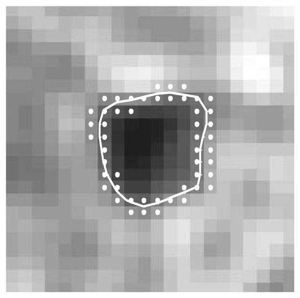
Zero level set contour (white) with a chosen narrow band (white dots).

5. Experimental details

Our institutional review board approved this study. We analyzed 233 liver lesions divided into two subsets. The first subset contains 69 lesions, obtained from 69 contrast-enhanced CT images of distinct patients (Siemens Medical Solutions, Erlangen, Germany). This subset, which was obtained at Stanford Medical Center, includes 20 hemangiomas, 25 cysts and 24 metastases liver lesions. The following image acquisition parameters were used: 120 kVp, 140–400 mAs, 2.5–5 mm section thickness and pixel spacing of 0.729 ± 0.072 mm (min - 0.684 mm, median - 0.784 mm, and max – 0.938 mm). All CT images have isotropic pixels. The second subset includes 164 liver lesions, obtained from 164 MRI images of 52 different patients scanned at a different academic institution (UC San Diego Medical Center). All patients underwent 3T gadoxetic acid enhanced MRI (Signa Excite HDxt; GE Healthcare, Milwaukee, WI) at a tertiary liver center for evaluation of suspected hepatocellular carcinoma (HCC) and were found to have one or more LI-RADS (LR) legions classified as LR-3 or LR-4. Slice thickness is 5 mm and pixel spacing is 0.804 ± 0.077 mm (min - 0.584 mm, median - 0.815 mm, and max – 0.945 mm). Similar to CT images, all MRI images have isotropic pixels. Pulse sequences of single-shot fast spin-echo T2-weighted, and pre- and post-contrast axial 3D T1-weighted fat-suppressed gradient-echo were used.

The different imaging modalities and clinical diagnoses result in high diversity of lesion characteristics present. A wide range of lesion sizes was found in the full set of 233 lesions. The size of CT liver lesions ranged from 18.58 × 20.20 mm to 125.24 × 132.15 mm. The MRI liver lesions ranged from 16.87 × 14.06 mm to 32.81 × 36.56 mm. Therefore, using a single fixed-size local window for all lesions may be inaccurate and will create an inconsistent segmentation performance, means that a specific window size will be good for some lesions, but for other it will not. A wide range of other spatial characteristics such as contrast and homogeneity illustrates the importance of, and need for, an adaptive local window size that is able to handle a wide range of spatial characteristics. These spatial criteria serve as key ideas for our method as given in equation (Fig. 5).

Fig. 5.

Spatial characteristics of the lesions (L) and the whole ROI (G).

Radiologists supplied two different types of manual annotations.

The first type manual annotation was a linear markup - two input points that represent the approximate long axis of the liver lesion. These two points were used as a diameter of a circle that we generated to provide an initial contour for the automated segmentation. Inter-reader variability of 2.87 mm ± 2.28 mm was found between the two input points supplied by the two radiologists. Therefore, to investigate the sensitivity of the segmentation to varied initializations that may be supplied by different radiologists, we changed the angle and length of the user-supplied linear markup. Five linear markups were generated for each lesion by randomly adjusting the position of the two input points within a 5-pixel diameter (~ 4 mm). A 5-pixel diameter was considered reasonable, based on intra-variability of radiologist annotations.

The second type of manual annotation provided was a complete manual segmentation of the entire lesion. It was used only for validating the final result of our automated segmentation. The automated segmentation contours were extracted and quantitatively compared with the average of the two radiologists’ marking.

6. Results

6.1. Segmentation performance

Cost function parameters of μ₁ = 0.15, λ₁ = 2, λ₂ = 2 were used, as they supplied the best average results for all 233 lesions. Figure 6 shows some examples of segmentation for different lesions. Segmentation performance was assessed using the Dice similarity coefficient (Table 1). The Dice coefficient was calculated relative to each radiologist’s manual marking, and then an average Dice score estimated. Our proposed segmentation method has high agreement with the manual markings for different local energies. Those results are better than the overlap that was measured between the complete manual annotations of both radiologists (average of 0.872, 95% CI of [0.863 0.88]), thus demonstrating the strength of our automated method. Non-significant differences were found between the average manual annotations and the automated segmentations (Wilcoxon, p>0.05), thus the manual marking can be replaced by the automated one.

Fig. 6.

Automatic segmentations (yellow) of liver lesions in CT (a–d, f) and MRI (e, g–i) images obtained using the ALW method with the piecewise constant model (PC). (a–b) different lesion sizes (Dice of 0.88, 0.91 respectively), (b–d) heterogeneous lesions (Dice of 0.91,0.92, and 0.89, respectively), (e) homogeneous lesion (Dice of 0.97), (f–g) low contrast lesions (Dice of 0.92, and 0.96 respectively), (h–i) noisy background (Dice of 0.93, 0.86 respectively). Green contours represent the manual annotations.

Table 1.

Average dice coefficient and 95% confidence interval (CI) for the lesion analysis using the proposed adaptive local window compared to manual marking.

	ALW VS. Manual marking [95% CI]
PC energy	0.89 [0.88, 0.90]
MS energy	0.87 [0.86, 0.88]
HS energy	0.88 [0.87, 0.89]

6.2. Process convergence

Figure 7 demonstrates the convergence of both the Dice coefficient and the energy functional over multiple iterations. For both CT and MRI images, the Dice coefficient increased rapidly over a few iterations as the automated segmentation converged on a result that matched the manual segmentations. As expected, energy decreased with increasing iterations, converging on a single value; this implies minimization of the energy functional. For both metrics, substantial convergence was obtained after fewer than 20 iterations and there were only minor fluctuations around their final values over later iterations.

Fig. 7.

Convergence of the (a) Dice coefficient and the (b) energy functional over iterations for both MRI and CT datasets.

6.3. Comparison with global energy

We compared our method with the PC global energy model of Chan and Vese (2001), using the same μ, λ₁, and λ₂ parameter values as we used for our ALW method. The global energy model and manual marking had a mean overlap (Dice similarity coefficient) of 0.784, with a 95% Confidence Interval of [0.759–0.805]. This is significantly less than the 0.89 Dice coefficient obtained using ALW for the local PC energy model (Wilcoxon, p < 0.001). Figure 8 reveals that the global energy model shows poor agreement with manual marking when analyzing images with low contrast (Fig. 8a–8c) or heterogeneous lesions (Fig. 8d–8f), especially if the lesions are located near the boundaries of the liver itself (Fig. 8e).

Fig. 8.

Examples for contours that were obtained by the manual marking (green contour), the proposed ALW (yellow contour) and the global PC energy (magenta contour). Parts of the magenta contour, which are seen as a straight line, represent excessive curve evolution that was stopped by the borders of the selected ROI bounding box.

6.4. Comparison with fixed square local window

We also compared our ALW with a common-used method that uses a fixed square local window (FLW) surrounding each contour point. The comparison was done for each of the three local energy models – PC, MS and HS. As with the ALW and global energy models, the same parameter values (μ₁ = 0.15, λ₁ = 2, λ₂ = 2) were used because they supplied the best results on average for all 233 lesions. Thus, the only difference between the FLW and the ALW methods was the size of the local window in which the statistics were calculated. Hence, any difference in performance was directly related to the local window size. For FLW, we began by testing a range of window sizes from 4 mm to 20 mm. For CT lesions, 11 mm square windows gave the best average performance, and for MRI liver lesions, 9 mm square windows were best. Therefore, these two fixed sizes were used for the FLW method. For all 233 lesions, the 9 mm square window gave an average Dice coefficient of 0.851(95% CI: 0.84–0.86) for all three local energy models. Using a 11 mm square window, the mean Dice coefficient was 0.83 (95% CI: 0.81–0.85). For each applied energy model, the performance of ALW was significantly better than FLW with each of those fixed radii (Wilcoxon, p < 0.01). Figure 9 shows six different lesions that demonstrate segmentation challenges and reveal that our ALW can handle these diverse types of images better than local FLW segmentation. The superiority of the adaptive method can be seen for each of the three energy models tested (PC, MS and HS).

Fig. 9.

Examples for contours that were obtained by the manual marking (green contour), the proposed ALW (yellow contour) and the FLW method (magenta contour). (a) PC model – CT liver lesion, (b) PC model – MRI liver lesion, (c) Mean separation (MS) model – MRI liver lesion, (d) Mean separation (MS) model – CT liver lesion (e) Histogram separation (HS) model – CT liver lesions, (f) Histogram separation (HS) model – MRI liver lesions.

Subset of lesions for which one or more automated methods (ALW or FLW) had less than 70% agreement with the manual marking were also examined separately (Fig. 10). Significant Dice improvement of 0.19 ± 0.09 was obtained for this subset by using our ALW (Wilcoxon, p < 0.05 for PC model, p < 0.001 for MS and HS models), compared with the classic FLW.

Fig. 10.

Subset of lesions, for which one or more automated methods obtained less than 70% agreement with the manual marking. For FLW, 9 mm and 11 mm window sizes were used. Comparison was performed for all

A second subset of lesions that had performance differences between ALW and FLW of greater than 10% was also considered. The 10% difference was chosen according to clinical decision, wherein ALW could be better or worse than FLW. Table 2 shows that our ALW outperforms FLW for each of the local energy models, with a significant mean performance improvement of 0.25 ± 0.13 (Wilcoxon, p < 0.001 for all three energy models). Moreover, ALW shows lower sensitivity and smaller dependence on a specific local energy than FLW.

Table 2.

Subset of lesions for which absolute performance differences higher than 10% between ALW and FLW was obtained. Dice coefficient is presented. Wilcoxon paired test was performed between the ALW and each FLW (p < 0.001).

	Number of Lesions	Number of Lesions
	ALW [95% CI], FLW9 [95% CI]	ALW [95% CI], FLW11 [95% CI]
PC	11	18
	0.84[0.77, 0.89]	0.83 [0.79, 0.87]
	0.70 [0.63, 0.8]	0.72 [0.64, 0.8]
MS	42	60
	0.84 [0.79, 0.85]	0.85 [0.81, 0.86]
	0.54 [0.47, 0.59]	0.47 [0.41, 0.52]
HS	25	60
	0.82 [0.80, 0.85]	0.83 [0.78, 0.86]
	0.60 [0.55, 0.64]	0.59 [0.54, 0.64]

6.5. Comparison with region-scalable fitting (RSF) model

We compared our method to an additional local level set approach (Li et al., 2008). The authors propose a region-scalable fitting (RSF) model. In their work, the authors present weighted averages of the image intensities in a Gaussian window inside and outside the contour. Therefore, the authors claimed that their method is better than FLW for cases with high spatial inhomogeneity, which is a challenge that appears in our dataset. However, as with the FLW method presented above, RSF method still requires user input - pre-definition of the values of local scales that can be applied. In their method, three different scales were tested and a specific one was manually fitted for each type of lesions according to a visual qualitative analysis of the lesions’ spatial characteristics. The chosen scale was fixed for all contour points and over iterations. The inefficiency and the inaccuracy of the manual tuning enhance the added value of our adaptive ALW method that fitted different window sizes for different lesions, contour points and over iterations, without any required input of those scales. We tested Li’s RSF method on both the MRI and CT datasets across all initializations. In order to conduct an optimal evaluation of the RSF method, we analyzed our lesions using a range of Gaussian scales (0.5:0.5:4). Li et al. used only 3 tested scales; therefore our RSF validation should be even more accurate. Values to the left and right of this range resulted in worse segmentation performance and convergence of the contour into local minima and increased sensitivity to noise. The best Gaussian scale was then chosen for each lesion. In addition, several values of λ₁ and λ₂ were tested, and λ₁=λ₂=2 was found to yield the best average results. Li’s method supplied an average Dice of 0.88± 0.06 for the entire dataset of 233 lesions. Thus, the segmentation results obtained by the RSF method are comparable to the traditional FLW results (p>0.05, Wilcoxon) but still worse than our ALW results.

6.6. Sensitivity to parameters

Only one parameter is required for the decision of the local window size - the distance between each pair of pixels used for calculating the GLCM matrices. We tested distances of 1, 2, 3, 4 and 5 pixels before choosing the 1-pixel distance as best. All 233 lesions and all tested distances combined had an average Dice coefficient of 0.887 ± 0.004. The negligible standard deviation indicates that the segmentation performance is affected very little by the value of this parameter. Thus, the performance of our method is stable, and the parameter does not need to be re-tuned manually for different populations of lesions.

6.7. Sensitivity to initialization

We assessed the ability of our model to deal with deviations in the positioning of the initial contour by applying five randomly different contour initializations. Results demonstrate that the ALW method supplied the highest Dice similarity values, compared with both FLW fixed window sizes and with the RSF model. Table 3 shows the average performance of ALW, and FLW when using five different contour initializations. The ALW showed better agreement with the manual marking and smaller changes in the segmentation performance when it was applied using different local energy models, significantly better than FLW windows (Wilcoxon, p < 0.05 for PC model, p < 0.001 for MS and HS models). When the RSF model was applied, an average Dice coefficient of 0.84 with 95% CI of [0.83, 0.85] was obtained, for all contour initializations. The RSF showed comparable results to the FLW method, but with smaller CI, suggesting that the RSF model is more robust than the FLW. However, those values are still significantly lower than our ALW performance (Wilcoxon, p < 0.05). Figure 11 presents two representative images to show this result visually. Each image contains two inaccurate long-axis points that lead to reconstruction of an inaccurate initial contour. The results reveal that despite with noise (Fig. 11a) and low contrast lesions (Fig. 11b), our model can deal with substantial deviations of the location of the initial contour.

Table 3.

Segmentation performance (mean Dice coefficient for comparison with manual marking) for the proposed ALW and the classic FLW at two different fixed sizes: 9 mm square (FLW9) and 11 mm square (FLW11). Results from five different contour initializations were averaged. Three different energy models were used.

	PC (N=233) [95% CI]	MS (N=233) [95% CI]	HS (N=233) [95% CI]
ALW	0.885 [0.88, 0.89]	0.86 [0.85, 0.86]	0.87 [0.87, 0.88]
FLR9	0.878 [0.87, 0.88]	0.82 [0.81, 0.83]	0.85 [0.84, 0.87]
FLR11	0.88 [0.87, 0.88]	0.78 [0.77, 0.80]	0.83 [0.80, 0.86]

Fig. 11.

Inaccurate initialization and final segmentation. Both long-axis input points (white stars) and the initial contour (red circle) that was reconstructed due to those points are presented. The yellow contour in each image illustrates the final accurate segmentation of the lesion.

6.8. Computational time

We examined the computational time required by the proposed method to analyze each lesion. All data were processed using MATLAB R2013b 64–bit (MathWorks Inc., 2013). Compared to the time required by the FLW method, or proposed ALW model took 2–5 times (~20–60 s) longer to run on the same hardware.

7. Discussion and conclusions

We present a novel method for adaptive re-estimation of the local window (ALW) for level set segmentations. The window is re-estimated 1) for each contour point, 2) separately for X and Y window dimensions, 3) over level set segmentation iterations, and 4) separately for each lesion in the dataset. The size of the local window is re-estimated based on 1) the size of the lesion, 2) the spatial texture, and 3) the minimization of the energy functional over iterations. The rationale for choosing those criteria is the substantial diversity of these lesion characteristics (Fig. 5).

Our method contains a local contrast term in addition to global criteria for contrast and homogeneity. The inclusion of both local and global criteria has an important benefit. We demonstrate that incorporating both global and local criteria correctly identifies the best local window size.

Our proposed method shows high agreement with expert manual marking for a diverse dataset of CT and MRI images (Fig. 6). The variety of spatial texture characteristics in our datasets emphasizes the strength of our adaptive method. Our ALW method performed well with low contrast images, heterogeneous lesions, and with noisy lesions or noisy backgrounds.

We compared our results to a global PC energy model (Fig. 8), to models using a pre-defined fixed local window size (Fig. 9), and to RSF model with scalable regions. Lankton and colleagues (Lankton et al., 2007; Lankton and Tannenbaum, 2008) note that their FLW model has high chances of breaking down in a set of widely varying lesions. Our results confirm that it is almost impossible to choose single fixed-size local window that will best fit every case (section 6.4). Among all fixed window sizes tested, a 9 mm square window was better for MRI lesions and a 11 mm square window was better for CT lesions. Estimating an adaptive local window using our method, results in a better agreement with traditional manual marking.

We analyzed two subsets of lesions based on results. Table 2 shows that for lesions with Dice differences higher than 10% between ALW and FLW, our ALW was significantly better. Dice similarity to manual marking was greater by 0.25 ± 0.13 (Wilcoxon, p < 0.001 for all 3 energy models). The second subset of lesions were those in which one or more automated methods obtained less than 70% agreement with the manual marking (Fig. 10). For this subset, the Dice coefficient with manual marking was improved by 0.19 ± 0.09 using ALW versus FLW (Wilcoxon, p < 0.05 for PC model, p < 0.001 for MS and HS models).

The method was also evaluated using five different contour initializations. Our ALW method performs better under these conditions than the FLW methods as it was affected less by different initial contour values (Table 3). The use of both local and global statistics in the model increases the segmentation agreement with the manual marking and by lowers dependence of the model on changes in the location of the initial contour.

We compared our method also to the RSF method. The RSF showed comparable results to the FLW method, after manually optimizing the local window sizes for each lesion separately. RSF showed performance that is more robust than the FLW across different contour initializations. Still, our ALW method produced higher agreement with the manual marking, as well as higher robustness across initializations, compared with the RSF model.

We also examined model sensitivity to parameters. Sensitivity to the single pre-defined parameter in the method - the distance between each pair of pixels used for calculating the GLCM matrices - was very low. Therefore, parameter tuning is not needed for the evaluation of the adaptive local window.

The presented work has some limitations. First, although our database of images of 233 lesions (69 CT, 164 MR) comes from two academic institutions, a larger sample size is desirable. Second, additional manual markings for each lesion may result in a more accurate evaluation of the automated segmentation.

Future work may include an automated evaluation of the level set parameters μ, λ₁, and λ₂. Extension of the method to 3D is also a future direction, as well as incorporation of automatic detection of the lesions prior to segmentation, so that the entire segmentation process is fully automated, with no dependence on user input.

In summary, the method presented shows significantly more accurate lesion segmentation than current state of the art level set methods. It performed better than prior methods in all tested configurations, including different local energy models, different contour initializations, and for different levels of lesion complexity.

Highlights.

• We improve the local level set segmentation by proposing a novel method to estimate the adaptive local window size surrounding each contour point.

• The local window size is re-estimated at each point by an iterative process that considers the object scale, local and global texture statistics, and minimization of the cost function, thus generating an adaptive local window.

• The proposed method estimates the size of the local window directly from the image, not by testing a specific scale from a range of scales and thus requires no pyramid of pre-defined scales as input, removing any potential sensitivity to user input regarding scale sizes.

• The results indicate that our proposed method outperforms the state of the art methods in terms of agreement with the manual marking and segmentation robustness to contour initialization or the energy model used. In case of complex lesions, such as low contrast lesions, heterogeneous lesions, or lesions with a noisy background, our method shows significantly better segmentation with an improvement of 0.25 ± 0.13 in Dice similarity coefficient, compared with state of the art fixed-size local windows (Wilcoxon, p < 0.001).

References

- Abdel-massieh NH, Hadhoud MM, Amin KM. A novel fully automatic technique for liver tumor segmentation from CT scans with knowledge-based constraints. Proceedings of 10th international conference on intelligent systems design and applications; 2010. pp. 1253–1258. [Google Scholar]
- An J, Rousson M, Xu C. Convergence approximation to piecewise smooth medical image segmentation. Proc Med Imag Comput Comp Assist Interven. 2007;(4792):495–502. doi: 10.1007/978-3-540-75759-7_60. [DOI] [PubMed] [Google Scholar]
- Ardon R, Cohen LD. Fast Constrained Surface Extraction by Minimal Paths. Int J Comput Vis. 2006;(69):127–136. [Google Scholar]
- Bhattacharyya A. On a measure of divergence between two statistical populations defined by their probability distributions, Bull. Calcutta Math Soc. 1943;(35):99–110. [Google Scholar]
- Cao L, Udupa JK, Odhnera D, Huanga L, Tonga Y, Torigiana DA. A General Approach to Liver Lesion Segmentation in CT Images. SPIE; 2016. [Google Scholar]
- Casciaro S, Franchini R, Massoptier L, Casciaro E, Conversano F, Malvasi A, Lay-Ekuakille A. Fully automatic segmentations of liver and hepatic tumors from 3-d computed tomography abdominal images: comparative evaluation of two automatic methods. IEEE Sens J. 2012;12(3):464–473. [Google Scholar]
- Caselles V, Kimmel R, Sapiro G. Geodesic active contours. Int J Comput Vision. 1997;22(1):61–79. [Google Scholar]
- Chan TF, Vese LA. Active contour without edges, IEEE Trans. Image Process. 2001;10(2):266–277. doi: 10.1109/83.902291. [DOI] [PubMed] [Google Scholar]
- Chan TF, Vese LA. A multiphase level set framework for image segmentation using the Mumford–Shah model. Int J Comput Vision. 2002;50:271–293. [Google Scholar]
- Chopp D. Computing Minimal Surfaces via Level Set Curvature Flow. J Comput Physics. 1993;106(1):77–91. [Google Scholar]
- Ciesielski KC, Udupa JK, Falcão AX, Miranda PAV. Fuzzy connectedness image segmentation in graph cut formulation: a linear time algorithm and a comparative analysis. J Math Imaging Vis Papers. 2012;44(3):375–398. [Google Scholar]
- Cohen LD, Kimmel R. Global Minimum for Active Contour Models: A Minimal Path Approach. Int J Comput Vis. 1997;24:57–78. [Google Scholar]
- Deng X, Du G. MICCAI Workshop Proceedings of 3D Segmentation in the Clinic: A Grand Challenge II – Liver Tumor Segmentation 2008 [Google Scholar]
- Foruzan AH, Chen YW. Improved segmentation of low-contrast lesions using sigmoid edge model. Int J Comput Assist Radiol Surg. 2015:1–17. doi: 10.1007/s11548-015-1323-x. [DOI] [PubMed] [Google Scholar]
- Freedman D, Zhang T. Interactive Graph Cut Based Segmentation with Shape Priors. Proc IEEE Conf CVPR. 2005;1:755–762. [Google Scholar]
- Freiman M, Cooper O, Lischinski D, Joskowicz L. Liver tumors segmentation from cta images using voxels classification and affinity constraint propagation. Int J Comput Assist Radiol Surg. 2011;6(2):247–255. doi: 10.1007/s11548-010-0497-5. [DOI] [PubMed] [Google Scholar]
- Ge X, Tian J. An automatic active contour model for multiple objects. Int Conf Pattern Recognition. 2002 unpublished. [Google Scholar]
- Häme Y, Pollari M. Semi-automatic liver tumor segmentation with hidden Markov measure field model and non-parametric distribution estimation. Medical Image Analysis. 2012;16(1):140–149. doi: 10.1016/j.media.2011.06.006. [DOI] [PubMed] [Google Scholar]
- He Y, Luo Y, Hu D. Semi-automatic initialization of gradient vector flow snakes. J Electron Imag. 2006;(15):043006. [Google Scholar]
- Haralick RM, Shanmugam K, Dinstein I. Textural Features for Image Classification. IEEE Transactions on Systems, Man and Cybernetics, SMC. 1973;3(6):610–620. [Google Scholar]
- Honeycutt CE, Plotnick R. Image analysis techniques and gray-level co-occurrence matrices GLCM for calculating bioturbation indices and characterizing biogenic sedimentary structures. Computers and Geosciences. 2008;34:1461–1472. [Google Scholar]
- Jolly M, Grady L. 3D general lesion segmentation in CT. IEEE ISBI. 2008:796–799. [Google Scholar]
- Kadoury S, Vorontsov E, Tang A. Metastatic liver tumour segmentation from discriminant grassmannian manifolds. Phys Med Biol. 2015;60(16):6459. doi: 10.1088/0031-9155/60/16/6459. [DOI] [PubMed] [Google Scholar]
- Krishnamurthy C, Rodriguez JJ, Gillies RJ. Snake-based liver lesion segmentation. 2004:187–191. [Google Scholar]
- Lankton S, Nain D, Yezzi A, Tannenbaum A. Hybrid geodesic region-based curve evolutions for image segmentation. Proc SPIE: Med Imag. 2007;6510:65104U. [Google Scholar]
- Lankton S, Tannenbaum A. Localizing region-based active Contours. IEEE Trans Image Process. 2008;17(11):2029–2039. doi: 10.1109/TIP.2008.2004611. [DOI] [PMC free article] [PubMed] [Google Scholar]
- Li C, Huang R, Ding Z, Gatenby JC, Metaxas DN, Gore JC. A level set method for image segmentation in the presence of intensity inhomogeneities with application to MRI. IEEE Trans Image Process. 2011;20(7):2007–2016. doi: 10.1109/TIP.2011.2146190. [DOI] [PMC free article] [PubMed] [Google Scholar]
- Li CM, Kao C, Gore J, Ding Z. Implicit active contours driven by local binary fitting energy. IEEE CVPR; 2007. [Google Scholar]
- Li CM, Kao C, Gore J, Ding Z. Minimization of region-scalable fitting energy for image segmentation. IEEE Trans Image Process. 2008;17:1940–1949. doi: 10.1109/TIP.2008.2002304. [DOI] [PMC free article] [PubMed] [Google Scholar]
- Li CM, Liu J, Fox MD. Segmentation of external force field for automatic initialization and splitting of snakes. Pattern Recognit. 2005;38:1947–1960. [Google Scholar]
- Li C, Wang X, Eberl S, Fulham M, Yin Y, Chen J, Feng DD. A likelihood and local constraint level set model for liver tumor segmentation from ct volumes. IEEE Trans Biomed Eng. 2013;60(10):2967–2977. doi: 10.1109/TBME.2013.2267212. [DOI] [PubMed] [Google Scholar]
- Li Y, Hara S, Shimura K. A machine learning approach for locating boundaries of liver tumors in CT images. Proceedings of ICPR. 2006:400–403. [Google Scholar]
- Li CM, Xu CY, Gui CF, Fox MD. Level set evolution without re-initialization: a new variational formulation. Proc IEEE CVPR. 2005:430–436. [Google Scholar]
- Li G, Chen X, Shi F, Zhu W, Tian J, Xiang D. Automatic liver segmentation based on shape constraints and deformable graph cut in ct images. IEEE Trans Image Process. 2015;24(12):5315–5329. doi: 10.1109/TIP.2015.2481326. [DOI] [PubMed] [Google Scholar]
- Linguraru MG, Richbourg WJ, Liu J, Watt JM, Pamulapati V, Wang S, Summers RM. Tumor burden analysis on computed tomography by automated liver and tumor segmentation. IEEE Trans Med Imaging. 2012;31(10):1965–1976. doi: 10.1109/TMI.2012.2211887. [DOI] [PMC free article] [PubMed] [Google Scholar]
- Malladi R, Sethian JA, Vemuri BC. Shape modeling with front propagation: a level set approach. IEEE Trans Pattern Anal. 1995;17:158–175. [Google Scholar]
- Masuda Y, Foruzan AH, Tateyama T, Chen YW. Automatic liver tumor detection using EM/MPM algorithm and shape information. Softw Eng Data Mining. 2010:692–695. [Google Scholar]
- Militzer A, Hager T, Jäger F, Tietjen C, Hornegger J. Automatic detection and segmentation of focal liver lesions in contrast enhanced CT images. 20th international conference on, pattern recognition; 2010. pp. 2524–2527. [Google Scholar]
- Moltz JH, Bornemann L, Kuhnigk JM, Dicken V, Peitgen E, Meier S, Bolte H, Fabel M, Bauknecht HC, Hittinger M, Kiessling A, Pusken M, Peitgen HO. Advanced segmentation techniques for lung nodules, liver metastases, and enlarged lymph nodes in CT scans. IEEE J Sel Topics Signal Process. 2009;3(1):122–134. [Google Scholar]
- Mumford D, Shah J. Optimal approximation by piecewise smooth function and associated variational problems. Commun Pur Appl Math. 1989;42:577–685. [Google Scholar]
- Neuenschwander W, Szekely PFG, Kubler O. Initializing snakes. IEEE CVPR; 1994. unpublished. [Google Scholar]
- Osher S, Sethian JA. Fronts propagating with curvature dependent speed: algorithms based on Hamilton–Jacobi formulations. J Comput Phys. 1998;79:12–49. [Google Scholar]
- Peng D, Merriman B, Osher S, Zhao H, Kang M. A PDE-based fast local level set model. J Comp Phys. 1999;155:410–438. [Google Scholar]
- Pescia D, Paragios N, Chemouny S. Automatic detection of liver tumors. Proceedings of the 2008 IEEE international symposium on biomedical imaging. 2008:672–675. [Google Scholar]
- Piovano J, Papadopoulo T. Local statistics based region segmentation with automatic scale selection. ECCV. 2008:486–499. [Google Scholar]
- Ronfard R. Region-based strategies for active contour models. Int J Comput Vision. 2002;46:223–247. [Google Scholar]
- Schwier M, Moltz JH, Peitgen HO. Object-based analysis of CT images for automatic detection and segmentation of hypodense liver lesions. Int J Comput Assist Radiol Surg. 2011;6(6):737–747. doi: 10.1007/s11548-011-0562-8. [DOI] [PubMed] [Google Scholar]
- Shimizu A, Narihira T, Furukawa D, Kobatake H, Nawano S, Shinozaki K. Ensemble segmentation using AdaBoost with application to liver lesion extraction from a CT volume. Workshop on 3D segmentation in the clinic: a grand challenge II, MICCAI.2008. [Google Scholar]
- Smeets D, Stijnen B, Loeckx D, De Dobbelaer B, Suetens P. Segmentation of liver metastases using a level set method with spiral-scanning technique and supervised fuzzy pixel classification. MICCAI Workshop on 3-D Segmentation in the Clinic: A Grand Challenge II.2008. [Google Scholar]
- Smeets D, Loeckx D, Stijnen B, De Dobbelaer B, Vandermeulen D, Suetens P. Semi-automatic level set segmentation of liver tumors combining a spiral scanning technique with supervised fuzzy pixel classification. Medical Image Analysis. 2010;14:13–20. doi: 10.1016/j.media.2009.09.002. [DOI] [PubMed] [Google Scholar]
- Tan Y, Schwartz LH, Zhao B. Segmentation of lung lesions on CT scans using watershed, active contours, and Markov random field. Med Phys. 2013;40(4):043502. doi: 10.1118/1.4793409. [DOI] [PMC free article] [PubMed] [Google Scholar]
- Tauber C, Batatia H, Ayache A. A general quasi-automatic initialization for snakes: Application to ultrasound images. IEEE Int Conf Image Processing. 2005 unpublished. [Google Scholar]
- Tsai A, Yezzi A, Wells W, Tempany C, Tucker D, Fan A, Grimson E, Willsky A. A shape based approach to curve evolution for segmentation of medical imagery. IEEE Trans Medical Imaging. 2003;22(2):137–154. doi: 10.1109/TMI.2002.808355. [DOI] [PubMed] [Google Scholar]
- Tsai A, Yezzi A, Willsky AS. Curve evolution implementation of the Mumford–Shah functional for image segmentation, denoising, interpolation, and magnification. IEEE Trans Image Process. 2001;10:1169–1186. doi: 10.1109/83.935033. [DOI] [PubMed] [Google Scholar]
- Wang L, Macione J, Sun Q, Xia D, Li C. Level set segmentation based on local Gaussian distribution fitting. Asian Conference on Computer Vision. 2009:293–302. [Google Scholar]
- Wang X, Georganas ND. GLCM texture based fractal model for evaluating fabric surface roughness. Proceedings of the Canadian Conf El Comp En. 2009:104–107. [Google Scholar]
- Wu D, Liu D, Suehling M, Tietjen C, Soza G, Zhou KS. Automatic detection of liver lesion from 3d computed tomography images. IEEE CVPR Workshops. 2012:31–37. [Google Scholar]
- Yan J, Schwartz LH, Zhao B. Semiautomatic segmentation of liver metastases on volumetric CT images. Med Phys. 2015;42:6283–6293. doi: 10.1118/1.4932365. [DOI] [PMC free article] [PubMed] [Google Scholar]
- Yang Q, Boukerroui D. Optimal spatial adaptation for local region-based active contours: An intersection of confidence intervals approach. IMAGAPP. 2011:87–93. [Google Scholar]
- Yezzi JA, Tsai A, Willsky A. A fully global approach to image segmentation via coupled curve evolution equations. J Vis Comm Image Rep. 2002;13(1):195–216. [Google Scholar]
- Yim PJ, Foran DJ. Volumetry of hepatic metastases in computed tomography using the watershed and active contour algorithms. Proceedings of the 16th IEEE Symposium on Computer-Based Medical Systems.2003. [Google Scholar]
- Zhang K, Song H, Zhang L. Active contours driven by local image fitting energy. Pattern Recognit. 2010;43(4):1199–1206. [Google Scholar]
- Zheng Q, Lu Z, Yang W, Zhang M, Feng Q, Chen W. A robust medical image segmentation model using KL distance and local neighborhood information. Comput Biol Med. 2013;43(5):459–470. doi: 10.1016/j.compbiomed.2013.01.002. [DOI] [PubMed] [Google Scholar]
- Zuiderveld K. Contrast limited adaptive histogram equalization. Graphics Gems IV: Academic Press Professional. 1994:474–485. [Google Scholar]