Global water cycle and the coevolution of the Earth’s interior and surface environment

Abstract

The bulk Earth composition contains probably less than 0.3% of water, but this trace amount of water can affect the long-term evolution of the Earth in a number of different ways. The foremost issue is the occurrence of plate tectonics, which governs almost all aspects of the Earth system, and the presence of water could either promote or hinder the operation of plate tectonics, depending on where water resides. The global water cycle, which circulates surface water into the deep mantle and back to the surface again, could thus have played a critical role in the Earth’s history. In this contribution, we first review the present-day water cycle and discuss its uncertainty as well as its secular variation. If the continental freeboard has been roughly constant since the Early Proterozoic, model results suggest long-term net water influx from the surface to the mantle, which is estimated to be 3−4.5×10¹⁴ g yr⁻¹ on the billion years time scale. We survey geological and geochemical observations relevant to the emergence of continents above the sea level as well as the nature of Precambrian plate tectonics. The global water cycle is suggested to have been dominated by regassing, and its implications for geochemical cycles and atmospheric evolution are also discussed.

This article is part of the themed issue ‘The origin, history and role of water in the evolution of the inner Solar System’.

1. Introduction

The presence of liquid water on the surface is one of the key characteristics that make the Earth a unique planet, and it is usually considered to be critical for a planet to be habitable [1]. Also, surface water is often believed to be essential for the operation of plate tectonics [2], which in turn enables the return of surface water to the planetary interior. The amount of surface water is thus a time-dependent variable that is controlled by the dynamics of the Earth’s interior. The Earth not only has surface water but also has just a right amount of it to allow the subaerial exposure of continental crust, which is important for the modulation of the atmospheric composition as well as various biogeochemical cycles [3,4]. To better understand the role of water in the Earth’s history, therefore, we need to decipher how the distribution of water between the surface and the deep interior has changed with time and how it has affected the surface environment.

In this contribution, we focus on reconstructing the history of surface water by assembling relevant observational constraints and theoretical considerations. Water must have played important roles in the generation of plate tectonics [2], the formation of continental crust [5] and the emergence of life [1], but it is still too early to discuss these issues on a quantitative basis. By contrast, it is possible to derive a fairly robust constraint on the rough history of surface water, at least back to approximately 3 Ga, and we believe it worthwhile to explore its implications for the coevolution of the Earth’s interior and surface environment.

The structure of this paper is as follows. We start with what we know best, i.e. the present-day water contents of different reservoirs and water fluxes among them. Based on available geochemical and geophysical observations, we have to conclude that even the present-day water cycle is quite uncertain, but we then show that the constancy of continental freeboard provides a simple yet robust geometrical constraint on the history of surface water and thus the net water transport between the surface and the interior. Geological observations pertinent to the evolution of global water cycle are discussed in the light of this freeboard constraint. We also discuss the geochemical and geodynamical implications of the estimated history of surface water, and close with possible future directions.

2. Present-day global water cycle

(a). Water budget

We consider the following four reservoirs: the oceans (within which we include water in the atmosphere), the continental crust, the mantle and the core. The amounts of water in the first two reservoirs are best understood; the oceans and the continental crust contain, respectively, approximately 1.4×10²¹ kg and approximately 2.7×10²⁰ kg of water [6]. Most of water in the continental crust (approx. 87%) is contained in sedimentary rocks, with the remaining in metamorphic rocks. Herein we refer to 1.4×10²¹ kg of water as 1 ocean.

Water content in the mantle is more uncertain. The mantle is usually considered to consist of at least two different components: the depleted source region for normal mid-ocean ridge basalts (N-MORB) and the more enriched source region for enriched MORB (E-MORB) and oceanic island basalts (OIB). Analyses of those basalts indicate that the former contains approximately 100–200 ppm H₂O [7,8] whereas the latter carries approximately 300–900 ppm H₂O [7,9–12]. The relative proportion of these two components has been controversial, with the estimated fraction of the depleted MORB source mantle ranging from 30% to 90% [13–15]. This issue hinges critically on the composition of the bulk silicate earth (BSE), which plays the central role in any global mass balance calculation, and the uncertainty of BSE composition is such that the enriched source mantle could be volumetrically insignificant [16,17]. Assuming the mean water content of 150 ppm for the MORB source mantle and that of 600 ppm for the OIB source mantle, for example, the total water content of the mantle ranges from 1.3 ocean (30% MORB source) to 0.56 ocean (90% MORB source).

Some authors propose much higher water contents in the mantle, though their reliability is unclear. Marty [18], for example, derived 10±5 ocean water in the mantle by combining the mean mantle H/C mass ratio (0.99±0.42 [19]), the whole mantle C/N ratio (532±224 [20]) and the silicate Earth N/⁴⁰Ar ratio (160±40 [21]) with the ⁴⁰Ar abundance in the mantle (2.3±0.8×10¹⁸ mol). This estimate has several issues. First, the ⁴⁰Ar abundance used is based on the K/U ratio of 13 800 [22] and the BSE U content of 20±8 ppb [23], but more comprehensive analyses suggest lower values: approximately 12 300 [24] for K/U, and 17±6 ppb for the BSE U [16]. Second, the whole mantle C/N ratio of 532±224 was supposedly derived from C/N ratios for three kinds of MORB [20]: 273±106 (N-MORB), 433±392 (T-MORB, which is an intermediate type between N-MORB and E-MORB), and 1839±641 (E-MORB), but the range of the whole mantle ratio is clearly incapable of encompassing these individual ratios. Finally, and most important, the adopted mantle H/C mass ratio (0.99±0.42) was derived with estimates for the mantle H and C contents [19]. Hirschmann & Dasgupta [19] generated a number of different combinations of the MORB-source mantle and the OIB-source mantle by Monte Carlo sampling, from which they derived statistical estimates on the mantle H, C and H/C. Their Monte Carlo simulation yields the mantle water content ranging from 0.2 to 1.6 ocean mass. Using their estimate on the mantle H/C is thus equivalent to adapting their estimate on the mantle H, and there would be no need to go through multiple elemental ratios. The large discrepancy in the estimated mantle water content between Marty [18] and Hirschmann & Dasgupta [19] suggests that the particular combination of elemental ratios used by the former may be troublesome. Indeed, the combination of H/C, C/N and N/⁴⁰Ar is equivalent to H/⁴⁰Ar, and it is not known whether the H/⁴⁰Ar ratio is sufficiently uniform among MORB and OIB to allow the estimate of the mantle H content using the mantle ⁴⁰Ar value. We note that a related elemental ratio, K₂O/H₂O, is known to be highly variable among MORB and OIB, ranging approximately from 0.2 to 1.3 [7,25]. This wide range of K₂O/H₂O has been attributed to source heterogeneities [7] as well as a potential decoupling between K₂O and H₂O during melting [9]. An approach based on multiple elemental ratios seems to require greater care than usually given.

The distribution of water in the mantle may also be estimated more directly by geophysical means, e.g. interpreting seismic wave attenuation and electrical conductivity [26]. Such geophysical variables, however, still suffer from low spatial resolution and non-uniqueness, and interpreting them is also difficult owing to the paucity of reliable experimental data. In the case of electrical conductivity, for example, using different datasets or different inverse methods gives rise to disparate estimates [27], and even for the same conductivity profile, the implication for water content can be drastically different, depending on the choice of experimental dataset [28,29].

The amount of water in the core is practically unconstrained. The density of the Earth’s core is estimated to be 5–10 wt% lighter than that expected for pure iron [30,31], and this density deficit calls for the presence of light elements in the core. If one tries to explain the density deficit solely by hydrogen, it is possible to have up to approximately 100 oceans-worth of hydrogen in the core [32]. The core is, however, a very popular place for also other proposed light elements (e.g. S, Si and O) [33,34], and one composition model suggests 0.06 wt% H in the core [33], amounting to only approximately 8 oceans. Nevertheless, even this estimate is still much higher than the water mass in the mantle, and the majority of the Earth’s water could reside in the core. How much of water could have been dissolved into the core depends on the details of core formation [35], which remain largely unresolved. An attempt to track the distribution of water starting from the beginning of the Earth’s history is therefore unpromising at the moment, and this is why we place an emphasis on reconstructing the history of water backward in time (§3).

(b). Water fluxes

As the amount of water presently contained in the continental crust is small with respect to those in other reservoirs, there are two major water fluxes: (i) between the oceans and the mantle, and (ii) between the mantle and the core. The latter flux is uncertain but probably small because it is likely to be diffusion-limited. The direction of water flux at the core-mantle boundary depends on the partition coefficient of water between metallic and silicate phases, and given the potentially high water solubility of the core, the core may serve as a sink for mantle water [35]. In the following, we limit ourselves on the water flux between the oceans and the mantle.

Water is continuously carried from the mantle to the oceans by magmatism, and it is also returned to the mantle by subduction in the form of sediments and hydrated lithosphere. The consideration of various sources and sinks for the surface water has long indicated that the sum of sinks exceeds substantially that of sources [36,37]. A compilation by Ito et al. [36], for example, suggests that the magmatic H₂O input from mid-ocean ridges, hotspots and arcs combined amounts to , whereas the H₂O loss by the subduction of altered oceanic crust alone is 8.8±2.9×10¹⁴ g yr⁻¹. A more recent compilation by Jarrard [37] indicates that the global flux of subducted water (by sediments and oceanic crust) is 1.83×10¹⁵ g yr⁻¹. Part of this water flux, however, may be returned to the oceans by (non-magmatic) updip transport [38], and the H₂O input by arc magmatism is highly uncertain and may be as large as 6×10¹⁴ g yr⁻¹ [37]. Although the apparent flux of subducted water could be further increased if the subducting mantle is serpentinized [39], considerable uncertainty associated with updip transport and arc magmatism makes it difficult to estimate the net flux of subducted water.

Many previous studies on net water flux have suggested that too high net flux would cause too large a change in the global sea level to be consistent with observations. Ito et al. [36] estimated the net water flux into the mantle as 1.2−11×10¹⁴ g yr⁻¹, but they felt that the higher rates in this range were geologically unrealistic and suggested that the rate of 1−3×10¹⁴ g yr⁻¹ might be acceptable, if it were only for periods of 100 Myr or so. Similarly, a more recent study [40] suggests that the long-term net water influx should be less than 1×10¹⁴ g yr⁻¹ to keep the sea-level change below 100 m over the Phanerozoic. The consideration of sea level in these studies, however, usually assumes that the present-day hypsometry also applies to the past. This assumption is difficult to justify because the surface topography of the Earth has gradually been modified by the thermal and chemical evolution of its interior. In fact, substantial water influx is possible without causing any change in the sea level, as shown in the next section.

3. The secular evolution of water budget and the emergence of continents

(a). Eustasy and continental freeboard

After the rise of atmospheric oxygen at approximately 2.4 Ga, hydrogen escape into space became trivial [41], and the amount of surface water has been subject to a dynamic balance between volcanic degassing and subduction. There is no a priori need for the volume of water in the oceans to stay constant, and the distribution of water among different reservoirs could also change. Even if the volume of water in the oceans remained the same, the Earth’s hypsometry is time-dependent because of continental growth and the secular cooling of the mantle, and the area of oceans (or equivalently, the area of dry landmasses) could vary with time. As a prime example to illustrate the role of water in the Earth’s history, we will focus on the area of continental crust above the sea level in this section. It is an important variable for the surface environment, controlling the rate of chemical weathering and nutrient fluxes to the oceans as well as the planetary albedo.

The relative height of the mean continental landmasses with respect to the sea level is known as the continental freeboard, and abundant sedimentary records on continents suggest that the freeboard must have been close to zero at least during the Phanerozoic [42]. This constancy of the continental freeboard has been used to constrain continental growth [42–44], the cooling rate of the mantle [45] and ocean volume change [46,47]. Freeboard modelling boils down to a simple isostatic balance, but because it involves several components (figure 1), all of which can change with time, it is not a trivial exercise. Whereas previous studies on freeboard assumed at least one of those components to be constant, we will consider the possibility of temporal variation for all components (table 1), by reviewing relevant geophysical and geological observations. In particular, our modelling includes the secular evolution of continental lithospheric mantle, which is absent from previous freeboard studies.

Figure 1.

Schematic for the set-up of freeboard modelling. (a) The top part of the model. The zero-height continental section corresponds to where the present-day sea-level crosses continental topography. A positive h reduces the area of exposed landmasses A_ex. (b) The entire model view. Note that in this paper we show the hypsometry of ocean basins in a reverse order (i.e. decreasing topography with increasing cumulative surface area) to indicate a likely passive margin structure.

Table 1.

Comparison of freeboard modelling studies.

author(s)	ρoc	hoc	ρol	hol	ρom	ρcc	hcc	zac	ρcl	hcl	Vbo
Wise [42]	Cc	C	—d	—	C	C	Ve	—	—	—	V
Schubert & Reymer [43]	—	—	—	—	C	C	V	—	—	—	C
Galer & Mezger [45]	C	V	—	—	C	C	V	—	—	—	V
Harrison [46]	C	C	—	—	C	V	C	—	—	—	V
Hynes [44]	V	V	V	V	C	C	V	—	—	—	C
Flament et al.[48]	C	V	—	—	C	C	V	V	—	—	C
this study	V	V	V	V	V	V	V	V	V	V	V

^aContinental topography (see equation (3.12)).

^bVolume of water in the oceans.

^cAssumed to be constant.

^dNot considered.

^eTreated as potentially variable with time.

We assume the following isostatic balance to hold between the zero-age oceanic section and the zero-height continental section:

3.1

where h is the sea level with respect to the present-day value, d₀ is the average depth of mid-ocean ridges, ρ_w is the density of sea water (1030 kg m⁻³), and ρ_i and h_i denote density and thickness, respectively, for oceanic crust (i=oc), depleted oceanic lithospheric mantle (ol), asthenospheric mantle (om), continental crust (cc) and continental lithospheric mantle (cl). Except for ρ_w, all variables can be a function of time. The zero-height continental section is at the present-day sea level; the relative location of zero-height section within the continental area does not change with time, regardless of sea-level change. The depth of compensation is taken at the base of continental lithosphere, which determines the thickness of asthenospheric mantle (h_om) in equation (3.1). Seafloor bathymetry is controlled by the thermal evolution of oceanic lithosphere, and continental topography in the past is modelled after its present-day form. The subsidence of seafloor away from the ridge axis is accommodated by the thickening of thermal lithosphere, continental topography is accompanied with the variation of continental crustal thickness (figure 1), and the isostatic balance is satisfied everywhere in our model. The sea level h is determined to be consistent with the volume of water in the oceans, which can change with time.

In our modelling, we use the sea level instead of the continental freeboard. The freeboard is defined as the the mean continental height with respect to the sea level, and because continental topography can change with time, it is cumbersome to use the freeboard as the main variable. The sea level is measured with respect to the present-day zero-height continental section, and the constancy of the freeboard is equivalent to that the sea level remaining close to the present-day value (less than 200 m during the Phanerozoic [49]).

In the subsequent sections, we first describe how individual components may change with time. Freeboard modelling is then conducted by starting from the present day to 3.5 Ga; for this time span, it is probably safe to assume the operation of plate tectonics [2], and our understanding of the likely secular variations of these components is particularly robust back to approximately 2.5 Ga and further back to 3.5 Ga with additional assumptions.

(b). Evolution of oceanic buoyancy

The characteristics of oceanic lithosphere, composed of oceanic crust and depleted oceanic lithospheric mantle, are a function of mantle potential temperature, T_p, so it is imperative to first understand the thermal history of the Earth’s mantle. How the mantle cools depends on the balance between surface heat loss, Q, and internal radiogenic heat production, H. A hotter mantle in the past has long been assumed to convect more vigorously with higher surface heat flux, but such scaling of mantle heat flux is also known to require considerably higher radiogenic heat production than suggested by geochemical data [50]. If a hotter mantle convects slower, e.g. by the effect of mantle melting on viscosity [51], it becomes possible to reconstruct a reasonable thermal history without violating geochemical constraints, and this alternative is more consistent with petrological data on the cooling history of the Earth’s upper mantle [52] (figure 2a). For the purpose of discussion, however, we consider the following two cases: faster plate tectonics with high heat production, and slower plate tectonics with low heat production (figure 2b,c). In either case, average plate velocity is related to mantle temperature and surface heat flux (excluding heat generation in continental crust) as [57]

3.2

for which we use the following present-day values: Q(0)=38 TW [47], T_p(0)=1350°C [53] and v(0)=5 cm yr⁻¹ [58].

Figure 2.

(a) Two contrasting thermal histories (blue for slower plate tectonics (PT) and green for faster plate tectonics in the past, both taken from [2]) compared with the variation of mantle potential temperatures estimated for the last 3.5 Gyr (dots) [52]. These estimates are based on the composition of primary melts for Precambrian non-arc basalts, and their overall trend converges smoothly to the potential temperature of present-day MORB source (approx. 1350°C [53]), supporting the interpretation that the non-arc basalts formed by the melting of ambient mantle. (b) Corresponding surface heat flux (solid) and internal heat production (dashed). (c) Corresponding plate velocity. (d) Continental growth models: [54] (yellow), [55] (black) and [56] (magenta).

We test three models of continental growth: the instantaneous growth model of Armstrong [54] and two more gradual growth models [55,56] (figure 2d). For any given time, the total area of continents is then calculated as

3.3

where m_cc denotes the mass of continental crust, and the total area of seafloor is given as A_o(t)=A_E−A_c(t), where A_E is the surface area of the Earth. For the area-age distribution of seafloor, we assume a triangular form:

3.4

where τ is the seafloor age and G(t) is the plate creation rate. This is a good approximation to the present-day situation and corresponds to subduction irrespective of seafloor age [59]. The maximum seafloor age is given by

3.5

where G(t)=G(0)v(0)/v(t) and G(0)=3.45 km² yr⁻¹.

Once the mantle temperature is given as a function of time, the thicknesses and densities of oceanic crust and depleted lithospheric mantle can be calculated by the model of decompressional mantle melting, and we use the parametrization of Korenaga [60] (figure 3). The density of asthenospheric mantle is also a function of temperature as

3.6

where ρ_om(T_p(0)) of 3300 kg m⁻³ and α of 3.5×10⁻⁵ K⁻¹ [61] are used. This value of thermal expansivity is appropriate for hot asthenospheric mantle; a value of 3×10⁻⁵ K⁻¹, commonly used for lithospheric mantle, requires the incomplete viscous relaxation that can take place only at low temperatures [62].

Figure 3.

(a) Thicknesses and (b) densities of oceanic crust (cyan) and depleted oceanic lithospheric mantle (blue) as a function of mantle potential temperature. After [60].

For the subsidence of seafloor, we test two possibilities: the half-space cooling model [63] and the plate model [64]. The bathymetry for half-space cooling may be expressed as

3.7

where the subsidence rate depends on mantle temperature as

3.8

and b(0)=323 m Ma^−1/2 [63]. For the plate model, we use the empirical fit by Stein & Stein [64]

3.9

where the bathymetry is in metre and the age is in million years ago. The plate model is a phenomenological model developed to fit the detail of present-day bathymetry, and it is not clear how it could vary for deeper times [65]. The use of the present-day plate model, however, still serves our purpose to test the model sensitivity to the age-depth relation of seafloor. The present-day zero-age depth d₀(0) is 2654 m for the half-space cooling model [63] and 2600 m for the plate model [64].

(c). Evolution of continental buoyancy

Unlike oceanic lithosphere, there is no simple genetic relation between mantle temperature and the physical properties of continental lithosphere, so we attempt to vary the buoyancy of continental lithosphere to be consistent with available constraints. First, the average thickness of continental crust is approximately 41 km at present [66]. Based on the regional metamorphic grade of current exposure in Archean greenstone belts, Galer & Mezger [45] estimated that the Archean crust could have been thicker by 5±2 km at approximatively 3 Ga. We thus consider two cases: constant h_cc and a greater h_cc in the past with the rate of 2 km Gyr⁻¹. The average density of continental crust has been estimated as 2830 kg m⁻³ [66], but this is based on a crude empirical correlation between seismic velocity and density, and ρ_cc can be anywhere approximatively between 2800 and 2900 kg m⁻³. We use ρ_cc(0) of 2880 kg m⁻³, to facilitate the interpretation of lithospheric mantle density (see below), and again, we consider two cases: (i) constant ρ_cc(0) and (ii) a gradually changing density as prescribed by

3.10

where f₁=(t−2)/1.5 where t is in giga-annum. The second case is an attempt to emulate the mafic to felsic transition across the Archean–Proterozoic boundary [67]; this formulation implies that the density is the same as oceanic crust for 3.5 Ga, and linearly shifts to that of modern continental crust by 2.0 Ga.

The present-day average thickness of continental lithospheric mantle is set to 200 km [68]. With ρ_cc(0) of 2880 kg m⁻³, then the present-day isostatic balance (equation (3.1)) yields ρ_cl(0) of 3338 kg m⁻³. The density excess of 38 kg m⁻³ with respect to the asthenospheric mantle is required to explain the present-day zero-age depth of seafloor, and it may be interpreted as the combination of thermal and chemical contributions. At present, the temperature at the continental Moho is approximately 500°C for the average continental heat flow of approximately 60 mW m⁻² [69], and that at the base of the continental lithosphere (i.e. 240 km depth) can be assumed to be approximately 1470°C, which corresponds to the potential temperature of 1350°C with the adiabatic gradient of 0.5 K km⁻¹. The continental lithospheric mantle is thus approximately 500 K colder than the asthenospheric mantle on average, which gives rise to the density excess of 58 kg m⁻³. At the same time, the continental lithospheric mantle is compositionally more buoyant than the asthenospheric mantle, and the deficit of 20 kg m⁻³, which is required to lower the excess of 58  kg m⁻³ to 38 kg m⁻³, implies that the Mg# (100×molar Mg/(Mg + Fe) of mantle composition) of the former is higher than that of the latter by approximately 1.3 on average [70,71]. This average Mg# difference appears reasonable; Mg# of the Phanerozoic lithospheric mantle is virtually indistinguishable from that of the asthenospheric mantle (approx. 89), whereas Mg# of the Archean lithospheric mantle is as high as approximately 93 [72]. The average Mg# difference may deviate approximately from 1.3 if we assume different density for continental crust or different thickness for lithospheric mantle, but an important point is that the effect of chemical buoyancy must always be considered. As we go deeper in time, the fraction of the depleted Archean lithosphere must increase, and we use the following function for ρ_cl:

3.11

where f₂=t/2.5 where t is in giga-annum and Δρ^A_cl describes how buoyant the continental lithospheric mantle would have been in the Archean. The continental Moho could have been as hot as 800°C due to increased radiogenic heat production [57], reducing negative thermal buoyancy. Combined with the positive chemical buoyancy caused by the high Mg# (−60 kg m⁻³), becomes negative, around −7 kg m⁻³. These calculations, however, cannot be very accurate because it is difficult to know how representative the Archean lithosphere that has survived to the present would be for the average continental lithosphere in the Archean. We thus test two values of : 0 kg m⁻³ and −5 kg m⁻³. The former corresponds to the isopycnic case where the thermal and chemical effects are cancelled out exactly. The above formulation assumes that the average continental lithospheric mantle in the Archean was as depleted as the mantle xenoliths of Archean ages observed today, and this assumption is consistent with existing hypotheses for the formation mechanism of cratonic lithosphere [73,74]. Equation (3.11) implies that the continental lithospheric mantle has been negatively buoyant for the past approximately 2 billion years, but this does not necessarily mean that the lithospheric mantle has been subject to convective instability; the high viscosity of dry, depleted lithosphere can easily sustain a gravitationally unstable configuration [75,76].

At present, the continental lithosphere of the Archean age is generally thicker than that of the Phanerozoic age [77], but for the same reason as above, it is not clear how we should vary the average thickness of continental lithospheric mantle with time. Numerical modelling studies usually show the gradual thinning of continental lithosphere by convective erosion [78,79], but the degree of thinning varies among different models. As the lower bound on continental buoyancy, therefore, we keep h_cl constant in this study. Any potential variation in h_cl may be considered to be effectively represented by the variation of ρ_cl, because it is the product of ρ_clh_cl that enters into the isostatic balance.

The present-day continental topography may be approximated as

3.12

where x is the cumulative fraction of surface area, and x_i’s and a_i’s are set as x₁=0.575, x₂=0.657, x₃=0.725, a₁=−18.18, a₂=27.36, a₃=−2.127, a₄=2.932, a₅=−2.642, a₆=3.642, a₇=4.5 and a₈=52.03. The first part corresponds to the continental slope, the second to the continental shelf, and the third to the subaerial crust. As the continental area changes with time, the horizontal scale of this topography is uniformly adjusted. The amplitude of subaerial topography is expected to be reduced in the past because of hotter geotherm [48], and the vertical scale of the subaerial topography is linearly decreased with time so that, at 2.5 Ga, the maximum height becomes only one-third of the present-day value. For comparison, we also test the case of no reduction in the vertical scale.

(d). Results of freeboard modelling

From the present-day hypsometry as described in the previous section, the volume of water in the oceans is calculated as 1.496×10¹⁸ m³ for the half-space cooling model, and 1.469×10¹⁸ m³ for the plate model. There are small discrepancies from the actual ocean volume of 1.335×10¹⁸ m³ [80], because both the area–age distribution and age–depth relation are simplified in our modelling. If there is non-zero water flux between the oceans and the mantle, the volume of water in the oceans can change with time, and for simplicity, we assume that the water influx is constant with time. We consider three cases: (i) zero net flux, (ii) 3×10¹⁴ g yr⁻¹ and (iii) 4.5×10¹⁴ g yr⁻¹. In the last two cases, the volume of water in the oceans at 2.5 Ga is higher than the present volume approximately by 50% and 70%, respectively.

Thus far we mentioned two thermal histories, three continental growth models, two seafloor subsidence models, two models each for the thickness and density of continental crust, two models of the Archean lithospheric density, two models of continental topography, and three models of ocean volume change. We evaluated all of 2⁶×3²=576 permutations, and some representative results are shown in figures 4 and 5.

Figure 4.

Representative results of freeboard modelling with slower plate tectonics in the past with the continental growth models of (a,d,g) Armstrong [54], (b,e,h) McLennan & Taylor [56] and (c,f,i) Campbell [55]. (a–c) Sea level, (d–f) the areal fraction (with respect to the Earth’s surface area) of exposed continents above sea level, and (g–i) the zero-age depth of seafloor. In all panels, thick black curves denote a reference case, which assumes the net water influx of 3×10¹⁴ g yr⁻¹, half-space cooling for seafloor subsidence, 5 km thicker continental crustal at 2.5 Ga, time-varying continental crust density, Δρ^A_cl of −5 kg m⁻³, and reduced continental topography in the past. Other curves denote sensitivity tests in which only one of those assumptions is modified: constant volume of water in the oceans (dashed cyan), the net water influx of 4.5×10¹⁴ g yr⁻¹ (solid cyan), the plate model for subsidence (dashed tan), constant continent crustal thickness (solid orange), constant continental crustal density (dashed orange), Δρ^A_cl of 0 kg m⁻³ (solid green) and constant continental topography (dashed orange). In (d–f), thick dotted curves denote the total areal fraction of continental crust for the reference case. Even when continental mass does not change, this fraction can vary if continental thickness changes. The ridge depth shown in (g–i) is d₀−h, i.e. the depth with respect to the sea level. The ridge shallowing for the case of constant ocean volume is caused by the lowering of the sea level. CL, continental lithosphere.

Figure 5.

Same as figure 4 but with faster plate tectonics in the past.

One of our main findings is that the net water influx of at least approximately 3×10¹⁴ g yr⁻¹ is required to satisfy the constancy of the freeboard, regardless of the choice of thermal evolution and continental growth. This may be quite surprising to those familiar with previous freeboard studies. For example, assuming the constant volume of water in the oceans, Schubert & Reymer [43] combined the constant freeboard with faster plate tectonics in the past to derive a continental growth model similar to that of McLennan & Taylor [56], and Hynes [44] made a similar argument to discount the instantaneous growth model of Armstrong [54]. Past oceanic lithosphere made from a hotter mantle must have been more buoyant than the present one (figure 3), so if the buoyancy of continental lithosphere did not change with time, seafloor would have been shallower. The constant freeboard would thus require that the continental area or the volume of water in the oceans be smaller in the past. The degree of chemical depletion in mantle xenoliths sampled from continental lithosphere, however, has long been known to exhibit secular evolution [77,81], which is incorporated in our model (equation (3.11)). Because of this, the relative buoyancy of continental lithosphere with respect to oceanic lithosphere is higher in the past, as clearly seen in the evolution of ridge depth (e.g. figure 4g–i). The use of lower average density for present-day continental crust or thinner present-day lithospheric thickness than adopted here would lead to even greater continental buoyancy in the past, so our particular model setting should be regarded as a conservative choice. The time-varying chemical buoyancy of continental lithosphere has not been considered in previous freeboard modelling, at least quantitatively. Armstrong [82] once noted the lack of consideration of continental lithospheric mantle in the usual treatment of freeboard modelling, and he argued that younger continental lithosphere in the past was likely to be thinner, which might permit his growth model. Unlike its oceanic counterpart, however, the thickness of continental lithosphere is not a thermal issue [83]; the time scale of thermal diffusion is only approximately 300 Myr for the length scale of 200 km. Thinner continental lithosphere in the past would also conflict with the antiquity of thick Archean cratonic lithosphere [73].

The most important free parameter in our freeboard modelling is net water influx from the oceans to the mantle, and all of the reference cases shown in figures 4 and 5 assume the net water influx of 3×10¹⁴ g yr⁻¹. Two other cases (0 and 4.5×10¹⁴ g yr⁻¹) are also shown for comparison. The calculated history of sea level or ridge depth is not so sensitive to other parameters, whose variability is more restricted compared to that of water flux. To maintain the present-day sea level for the past 2 Gyr, the net water influx must have been approximately 3×10¹⁴ g yr⁻¹ for the continental growth model of Armstrong [54] and approximately 4.5×10¹⁴ g yr⁻¹ for the other two growth models. Even greater influx would be necessary for more gradual continental growth models (e.g. [84,85]). These water flux estimates can be lowered to some extent by reducing continental buoyancy in the past, e.g. assuming constant crustal thickness and less depleted lithospheric mantle, but it appears nearly impossible to eliminate the need of positive water influx entirely. Various curves other than thick solid ones in figures 4 and 5 are shown to visualize the contributions of different factors, and most of them are not meant to be similarly valid alternatives. The constant thickness of continental crust, for example, is difficult to justify given that the Precambrian crust invariably experienced erosion, even after crustal stabilization [45], and the Archean bathymetry following the present-day plate model is similarly unlikely. The results shown in figures 4 and 5 may thus be interpreted chiefly as a function of ocean volume change.

The relative insensitivity to the type of thermal evolution, up to approximately 2.5 Ga, can be explained by the competing effects of mantle temperature and plate velocity. In the case of slower plate tectonics in the past, mantle temperature rises quickly as we go deeper in time (figure 2a), but plate velocity becomes lower (figure 2c), raising the maximum seafloor age. The former increases the chemical buoyancy of oceanic lithosphere, but the latter adds to its negative thermal buoyancy. In the case of faster plate tectonics, the rise of mantle temperature takes place more slowly, but plate velocity was faster, lowering the maximum seafloor age. These competing effects can be seen directly in the hypsometry snapshots (figure 6); in the case of faster plate tectonics, seafloor is much flatter, but its overall depth is also greater. Beyond approximately 2.5 Ga, two different thermal histories start to diverge because both mantle temperature and plate velocity rise very sharply in the case of faster plate tectonics.

Figure 6.

Hypsometry snapshots from the reference cases shown in figures 4 and 5 at present (solid), 1 Ga (green), 2 Ga (cyan) and 3 Ga (magenta). Corresponding sea levels are shown in dashed lines. The hypsometry is measured with respect to the (present day) zero-height continental section, the relative location of which in the continental area does not change with time (figure 1a). The absolute height of the reference point, with respect to the centre of the Earth, varies to satisfy the conservation of mass in the solid Earth.

Compared with sea level and ridge depth, the calculated history of the area of exposed continents (e.g. figure 4d–f) is sensitive to more parameters, except for the case of the continental growth model of McLennan & Taylor [56]. In this growth model, the continental mass changes drastically at 2.5 Ga, and the exposed continental area must follow this trend. In other growth models with more gradual (or no) variation in the continental mass across the Archean–Proterozoic boundary, the timing of the emergence of continents above the sea level is sensitive to subtle changes in a number of factors, including ocean volume, the thickness of continental crust and its density, seafloor bathymetry and continental topography. It is interesting to see that, even with the Armstrong growth model, the rapid emergence of continents around the Archean–Proterozoic boundary is possible (figures 4d and 5d). By contrast, the growth model of McLennan and Taylor makes it difficult to achieve a transition from the submarine to subaerial environment, because flooding becomes less likely with much reduced continental mass (i.e. broader ocean basins) before 2.5 Ga (figure 6c).

Though our freeboard modelling is more complete than previous attempts, it is still largely kinematic; some factors are simply assigned, rather than being solved in a self-consistent manner. For example, the thermal evolution of the mantle is likely to be coupled with net water influx, and so is the growth of continents. Also, the net water influx is assumed to be time-independent for the sake of simplicity. Our theoretical understanding of Earth evolution is such that it is more beneficial to explore the model space freely than to limit the model search by an imperfect theory. On the basis of existing geophysical and geological constraints, we believe that the end-member cases considered here should be able to encompass a realistic evolutionary scenario, and that the first-order features of modelling results are reasonably accurate.

4. Discussion

(a). Precambrian freeboard and emergence of continents

Although constraints on freeboard in the Precambrian are far less developed than in the Phanerozoic, there is still a suite of geologic and geochemical observations that provide insights into the early history of continental exposure. Cases have been made for near-constant freeboard through much of the Precambrian (e.g. [42,86]), but there are uncertainties and debate about most observations and proxies that are used to quantify the global extent of continental exposure. We will briefly review some of the commonly discussed means of tracking the history of sea level and also explore some non-traditional proxies.

Exposure surfaces (palaeosols) are the most intuitive observations that directly constrain the extent of continental exposure, but they provide very limited insights into the overall extent continental crust above sea level, given the elevation range within continental systems. However, nearly flat, laterally expansive (hundreds of square kilometres) exposure horizons may be able to provide insights into global-scale extent of exposure at given time in the Earth’s history. Although paleosols can be difficult to identify confidently in the Precambrian sedimentary record, intense, long-lived weathering surfaces can be identified (e.g. [87]). On the modern Earth, broad, level areas (plateaus) develop within mountain belts and can have elevation as high as 5 km. However, plateaus must be associated with an orogeny, and the basic tectonic setting of a region can be readily reconstructed from mapping and field observations, even in Archean terranes (e.g. [88]). Broad weathering surfaces with limited topographic relief that are not linked to an orogeny are likely to have formed less than 1 km above the sea level based on the modern hypsometry. Future work could move towards placing this idea into a more quantitative and rigorous model, but this rough framework can be used to do a first-pass exploration of the Precambrian record.

There are occurrences of spatially expansive exposure horizons in the Archean. Foremost, the ca 3.0 Ga Pongola–Witwatersrand Basin in South Africa contains several weathering horizons, one of which is spatially expansive. The most pronounced erosion surface in this succession is developed at the base of the sedimentary successions, with weathering occurring on underlying greenstone-granite basement. The exposure surface can be found in the Pongola and the Witwatersrand succession, spanning total area of hundreds of square kilometres. This palaeosol most likely represents an erosive surface that developed during subsidence of the craton around 3.1–3.0 Ga and is not linked to a major collisional event [89–91]. There is also a less spatially expansive exposure surface in the Pongola Supergroup between the contact of the Nsuze and Mozaan groups, but a conformable contact at the equivalent horizon in the Witwatersrand Basin. The exposure surface in the Pongola–Witwatersrand succession occurred on a stable cratonic basement, clearly not in a plateau setting. The 2.76 Ga weathering horizon on the Mount Roe Basalt in the Fortescue Group, Western Australia, was also recently recognized to be spatially widespread [92]. The Fortescue Group has been variably interpreted as a rift-to-passive margin sequence or as being part of a more complex, two-stage continental break-up [93,94]. Importantly, however, there is no evidence that the Fortescue Group deposition results from a major orogenic event. The Mount Roe Basalt is now restricted to palaeovalleys that existed on 2.78 Ga old peneplained surface, but this basalt and the exposure surface are likely to have also initially covered much of the craton [92]. There are numerous other Archean palaeosols, which future work may also determine are part of laterally extensive continental exposure surfaces. There are, however, no accepted or definitive palaeosols prior to 3.0 Ga (cf [87]).

Given the framework developed above about the significance of spatially expansive continental exposure surfaces, the Archean palaeosol records suggest the continental freeboard was roughly within a kilometre of modern values going back to the mid-Archean. Palaeosols are not a ubiquitous feature of the rock records, making it difficult to gauge if the ‘first appearance’ of widespread palaeosols at 3.0 Ga reflects environmental evolution or just a chance discovery in a sparse record. However, it is interesting to note that the first case in the rock record of widespread exposure surfaces occurs when there is a jump in our modelled extent of exposed continental landmass (figures 4 and 5). Whether or not the palaeosol record can pinpoint a transition in continental exposure, the occurrence of widespread palaeosols at 3.0 and 2.78 Ga (and younger times) support model results that suggest significant continental exposure over at least the last 3.0 Gyr. By contrast, the Archean palaeosol record appears to conflict with suggestions of limited (less than 5% of A_E) exposure throughout the Archean (e.g. [48]).

The broad-scale stacking patterns of volcano-sedimentary sequences can also be used to gauge the evolution of continental freeboard. Volcano-sedimentary sequences can, in principle, provide a record of a progressive flooding or prolonged exposure. A predominance of deep-water deposits and submarine volcanics (e.g. [95]) could point to higher sea level than what characterized the Phanerozoic. By contrast, a signature for periodic flooding of craton interiors is observed, and is consistent with limited average cratonic relief, similar to what was observed in the Phanerozoic. There are several Archean cratons (e.g. Kaapvaal and Pilbara) that are characterized by thick and cyclic epeiric marine deposits. The Kaapvaal and Pilbara cratons are also noteworthy in having extensive Archean–Paleoproterozoic sedimentary records, spanning from more than 3.0 Ga to less than 2.4 Ga. There are cratonic successions (e.g. the Abitibi Greenstone Belt on the Superior Craton) characterized by almost exclusively by deep-water facies (greywackes, black shales and submarine volcanics), which would be consistent with extensive cratonic flooding. However, the Abitibi Greenstone Belt (and other Archean succession lacking shallow water facies) are relatively short-lived, and extensive flooding is expected in certain tectonic settings (e.g. rift basins). In this light, the stacking patterns of volcano-sedimentary sequences do not provide precise freeboard estimates, but are most consistent with the persistence of significant continental exposure over the past 3 Gyr.

An extensive record of epicontinental flooding is recorded by terrestrial and marine basins developed on continental lithosphere, inboard of the continent-ocean margins. Figure 7 illustrates this record by graphically tabulating epicontinental basins from the last 3 Gyr, with areas greater than 30 000 km². The data are organized into cratonic areas identified within the Nuna, Rodinia and Gondwana/Pangea supercontinents [96] and categorized as either wholly terrestrial (typically fluvial), mixed terrestrial/marine or marine (usually shallow marine but sporadically including deep-water facies). The global record of epicontinental basins (figure 7) shows, foremost, that many cratonic regions experienced sporadic marine flooding or terrestrial cover in repeated episodes, rather than being continuously flooded or continuously unroofed and eroded. There is a tendency for epicontinental basins to become more rare in the deep past, which is probably attributable to a systematic decrease in sedimentary preservation with age. As second-order signals, both the prevalence of terrestrial settings for 1.8–1.6 Ga deposits and the lack of 1.0-Ga epicontinental basins may be related to the emergence and erosion of supercontinents Nuna and Rodinia, respectively. Several cratons, such as Laurentia, were episodically flooded and exposed repeatedly through the last 0.5 Gyr [97], indicating a remarkable stability in freeboard over that long interval. The same motif of episodic flooding is evident in the stratigraphic record of well-preserved Neoarchean–Paleoproterozoic cratons such as Laurentia, Kaapvaal (Kalahari) and Pilbara (Australia).

Figure 7.

Compilation of epicontinental sedimentary records for exposed areas larger than 30 000 km². The data are available from the authors upon request and will be described in detail in a forthcoming publication. Only broad trends are discussed herein.

The Sr isotope record has been extensively used to track the formation of continents and the exposure of continental crust. Specifically, there is a marine carbonate ⁸⁷Sr/⁸⁶Sr record with a Neoarchean (ca 2.7 Ga) rise in preferred ⁸⁷Sr/⁸⁶Sr ratios that has been variably proposed to track either the growth or the emergence of the continents [98,99]. The basic idea behind this is straightforward; more radiogenic seawater Sr isotope values can be confidently linked, through a global isotope mass balance, to the weathering of exposed continental crust, which is more radiogenic than the depleted mantle. However, tracking seawater Sr isotope values in Archean carbonates is not entirely straightforward. Radiogenic Sr isotope values can be derived from unintentional analysis of siliciclastic bound Sr. The convention has been to assume that the lowest ⁸⁷Sr/⁸⁶Sr ratios in a given time period are representative of seawater values. However, the diagenetic alteration of carbonates can also result in ‘low’ ⁸⁷Sr/⁸⁶Sr ratios if carbonates trap Sr acquired from the alteration of mafic rocks. In addition, a large amount of the Archean and Paleoproterozoic Sr isotope record has been generated with little or no complementary trace element data to track detrital contamination or carbonate alteration. Given the scarcity of Sr isotope data (relative to younger time intervals) and the variability in data quality, the conservative view would be that additional Sr isotope data is needed to provide compelling evidence for the onset of extensive continental exposure between 3.0 and 2.5 Ga. However, the traditional interpretation of the Sr isotope record is generally consistent with our modelling results, which also show an increase in extent of continental exposure at the end of the Archean (figures 4 and 5).

There is also a Neoproterozoic increase the observed minimum carbonate ⁸⁷Sr/⁸⁶Sr ratios [99] that, in the traditional framework, could be linked to an increase in the extent of continental exposure. A Neoproterozoic increase in continental exposure is difficult to reconcile with our freeboard model results. In fact, no model scenarios show a pronounced and sustained shift in continental exposure in the Neoproterozoic. Accumulation of radiogenic sedimentary Sr isotope values in the upper crust after extensive continental exposure should provide a ‘buffer’ that prevents swings to low seawater ⁸⁷Sr/⁸⁶Sr ratios during times of more limited continental input. This buffering mechanism should have become established 250 to 500 Myr (several half lives of the upper continental crust [100]) after extensive continental exposure (in the Late Archean in our results)—so at first glance this process is an unlikely explanation for the disagreement between the freeboard model results and the current carbonate Sr isotope curve. However, despite variability in the carbonate Sr curve through time, one could view the carbonate record as capturing a progressive increase in ⁸⁷Sr/⁸⁶Sr ratios—an increase driven by increasing radiogenicity of the upper continental crust. In addition to this protracted increase, ‘radiogenic sedimentary buffering’ would have progressively prevented dips to low seawater Sr isotope ratios during lulls in continental Sr input, potentially providing a means to reconcile our freeboard modelling with the observed Neoproterozoic–Phanerozoic increase in minimum carbonate ⁸⁷Sr/⁸⁶Sr ratios.

Non-traditional metal isotope proxies may provide a new means to track continental exposure. An initial sedimentary Zn isotope record (from iron formations) has been proposed to provide support for continental emergence at 2.7 Ga, consistent with the traditional view of the Sr isotope record introduced above [101]. However, we have a relatively limited understanding of Zn isotope cycling in iron-rich aqueous systems, opening up the possibility for alternative explanations of the limited amount Archean Zn isotope data generated thus far [101]. Osmium (Os), very similar to Sr, is part of a radiogenic isotope system (Re–Os) controlled by crustal differentiation and weathering of radiogenic continental crust. Therefore, the global Os isotope mass balance could, in theory, be used to track continental exposure. To date, the first notably radiogenic sedimentary Os isotope values are found at successions deposited near the end of the Archean (ca 2.5 Ga; [102]). However, Os is also redox sensitive, indicating that the late ‘first appearance’ of radiogenic sedimentary Os isotope values could be tied to atmospheric evolution (oxygenation) rather than continental exposure.

(b). Chemical weathering and atmospheric evolution

Changes in continental freeboard will have a large effect upon essentially all major biogeochemical cycles. This work was motivated in part by the desire to develop new estimates for exposed continental area and hypsometry through time that can be directly linked to various Earth surface biogeochemical models. However, herein we provide a qualitative discussion of how our freeboard estimates would have shaped the evolution of biogeochemical cycling (figure 8). More specifically, we discuss shifts in silicate weathering and phosphorus (P) fluxes to the oceans, the manner in which these shifts are linked to continental freeboard, and how these changes would have affected atmospheric oxygen and carbon dioxide levels.

Figure 8.

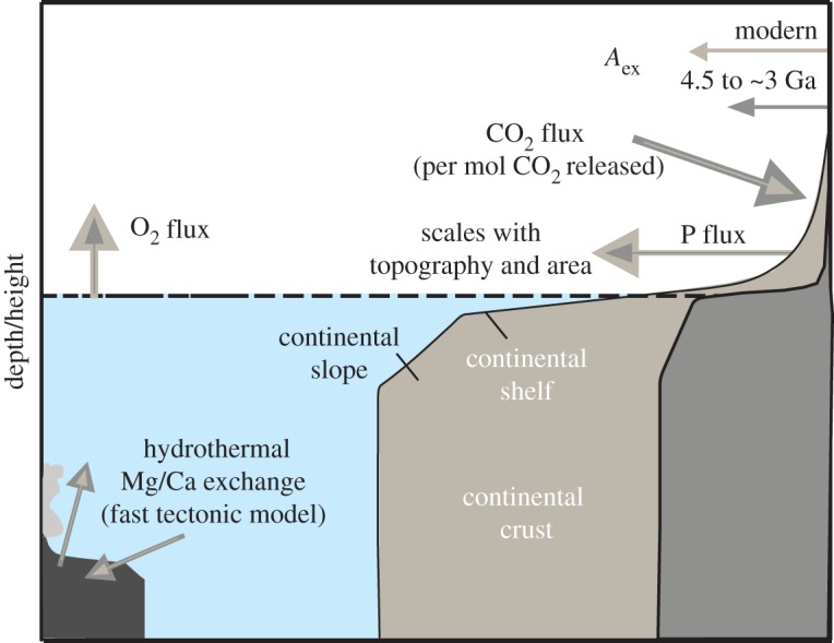
Schematic of the links between continental emergence and major biogeochemical cycles. The light grey area represents modern continental crust and fluxes and the dark grey represents the Archean continental crust and fluxes. Limited continental exposure might have lead to high weathering intensities in a CO₂ rich atmosphere and decreased phosphorus fluxes to the oceans. Lower phosphorous fluxes to the oceans would have limited primary productivity and oxygen release to the atmosphere. Traditionally, it was assumed there was greatly increased hydrothermal activity in the Archean, which would have reduced dissolved Mg levels, but there is no empirical support for this ‘fast tectonic’ model.

The central idea of the silicate weathering feedback [103,104] is that the extent of silicate weathering and thus CO₂ draw-down scales with temperature. Given that CO₂ is likely to have been a critical greenhouse gas over the past 4 Gyr, this temperature-dependent link is one of the main factors behind the Earth’s sustained habitability and persistently clement climate. However, the silicate weathering feedback, of course, only mitigates changes in carbon dioxide concentrations, and shifts in continental area and hypsometry will affect the efficiency of this feedback. With a constant CO₂ input the ocean–atmosphere system and with all other climate variables held constant, varying the extent of continental exposure will result in disparate globally averaged weathering intensities and different steady-state atmospheric CO₂ concentrations. With less continental exposure, more intensive silicate weathering per unit area is required to balance a given carbon dioxide input flux. Higher steady-state carbon dioxide concentrations are needed to drive higher weathering intensities (per unit area). In this light, the extent of continental exposure is likely to have been, over the past 4 billion years, an important driver of the Earth’s climate state and something that ought to be incorporated into discussion of Archean climate and the ‘faint young Sun paradox’ [105–107]. The steep increase in continental exposure from 3.0 to 2.4 Ga (figure 4) should also be taken into account when trying to quantify the factors responsible for the first appearance of ‘Snowball’-style low-latitude glaciation at 2.4 Ga [108]. Carbon cycle models, directly coupled to our geodynamic freeboard model, will be able to further explore the influence of freeboard evolution on Archean climate.

Phosphorus is commonly considered to the nutrient ultimately limiting primary productivity and thus life as a whole on the Earth. Continental weathering is the only significant source of P to the oceans. By strong contrast, nitrogen (N) can be biologically fixed in the marine system from a limitless supply of atmospheric N. Therefore, although N is commonly considered the ‘proximate’ limiting nutrient over large swaths of the modern oceans, P is typically considered to be the ‘ultimate’ limiting nutrient on geologically meaningful timescales [109]. Given that P is essentially sourced only from continental systems, the extent of continental exposure has the potential to dramatically alter the global P cycle, despite the potential for greater weathering intensities in Archean rocks (see above). Reduced continental exposure through the Archean, a feature observed in the vast majority of our model runs (figures 4 and 5), is therefore likely to have been a factor driving extremely low Archean C burial and thus atmospheric pO₂ levels (pO₂<10⁻⁷ to 10⁻⁵ PAL; [110]). Limiting primary productivity (via P scarcity) is the only feasible way to drive the ocean-atmosphere system to low atmospheric oxygen levels following the evolution of oxygenic photosynthesis [111], which multiple records indicate occurred by at least 3.0 Ga (e.g. [91,112]). Given that the O₂ sinks are smaller on an anoxic Earth and organic carbon burial is favoured in anoxic systems, low levels of primary productivity are likely an essential part of a low-oxygen ocean–atmosphere system [111,113]. On a similar note, the potential for a protracted rise of atmospheric oxygen from 3.0 to 2.4 Ga (e.g. [114]) could be due, in part, to gradual increases in the extent of continental area exposed (figures 4 and 5). By contrast, the presented freeboard modelling indicates that continental freeboard is not likely to have been a key factor responsible for the Neoproterozoic oxygen rise or low Proterozoic oxygen levels [114–116]. This indicates that inorganic marine P scavenging must be responsible for low Proterozoic atmospheric oxygen levels (e.g. [111]).

(c). Tempo of plate tectonics

The largest difference in continental freeboard estimates from our model using either ‘fast’ or ‘slow’ tectonics (see figure 2 for background on tectonic models) occur between 4.0 and 3.0 Ga, regardless of the used continental growth curve (cf. figures 4 and 5). Therefore, it is difficult to differentiate between these tectonic modes using empirical observations about the evolution of continental freeboard. The oldest siliciclastic sedimentary rocks on the Earth are more than 3.8 Ga [117], suggesting at least some degree of continental exposure in the Early Archean. However, the sedimentary record prior to 3.0 Ga is rather sparse. The ca 3.2 Ga Barberton Greenstone Belt contains thick shallow-water siliciclastic deposits, but it is difficult to gain much information about the global-scale extent of continental exposure from a single (e.g. localized) succession.

Observational support for the slow tectonic model has been mostly indirect, such as the thermal budget of the Earth [17], the lifespan of passive margins [118] and the cooling history of the upper mantle [52]. The tempo of plate tectonics can also be estimated directly from palaeomagnetic records of continental cratons, although there are important caveats. First, the direct application of palaeomagnetic data to reconstruct cratons suffers from a lack of control on palaeolongitude, given the rotational symmetry of the time-averaged field. Any palaeolatitude shift mandated by successive palaeomagnetic poles is thus a minimum estimate of the total motion of that craton. The issue can be overcome, somewhat, by applying a globally consistent kinematic model that includes palaeolongitude constraints [119–121]. ‘Absolute’ velocities of all continental blocks can be calculated for any such global model, even if its palaeolongitude framework is arbitrarily assigned [122]. However, such models still lack information on oceanic plates for pre-Mesozoic times; efforts to include such plates explicitly in the models are very laborious and introduce degrees of uncertainty that are difficult to quantify [123]. On top of all of these limitations, there is the additional fundamental uncertainty on whether to interpret continental motions as those of plates sliding over the asthenosphere, versus the entire mantle slipping over the core (true polar wander, TPW). It is likely that both plate tectonics and TPW occurred throughout the Earth’s history, but deconvolving the two factors from palaeomagnetically derived motions can be influenced strongly by data selection [124–127]. As one example, O’Neill et al. [128] purported to show prominent spikes in cratonic plate velocities at 1.1, 1.9, 2.2–2.1 and 2.7 Ga, but among those records, the alternative end-member TPW solution is either suggested directly by recent studies (1.1 Ga [129] and 1.9 Ga [130]), or made possible via recognition of rapid palaeomagnetic shifts on additional cratons (2.2–2.1 Ga, [131,132]), or presently untestable due to only one well-defined cratonic palaeomagnetic record at that age (2.7 Ga [133]). On a broader scale of analysis, the general trend of increasing continental plate velocities through time (twofold increase in the past 2 Ga) as suggested by Condie et al. [122] is mostly underpinned by very rapid motions through the Ediacaran–Ordovician interval, which have alternatively been interpreted as largely due to TPW [121,125,134,135], biases in the data due to rock-magnetic effects [136], or anomalous geomagnetic field behaviour [137–139]. If that unusual time interval is excluded from the analysis, then there is no significant trend in plate velocities through time. The most recent global kinematic model spanning the interval 2.0–1.3 Ga [140] produces a distribution of plate velocities with a peak only slightly lower (approx. 30%) than that of the Phanerozoic distribution; the slow tectonic model shown in figure 2b is consistent with such a modest change in globally averaged plate velocities.

Whereas palaeomagnetic constraints on oceanic plate velocities are difficult to obtain as mentioned, the Mg/Ca ratio of the Archean ocean may provide support for slower-spreading ocean ridges. Hydrothermal systems are characterized by Mg–Ca exchange (Mg removal) and it is possible to roughly link a seawater Mg/Ca ratio, to a range of hydrothermal Mg removal and continental Ca and Mg weathering fluxes [141]. In the Archean, the plate motion and heat generated by hydrothermal systems are much greater for the fast tectonic model than the slow tectonic model (figure 2b). For instance, the heat flux at 3.0 Ga in the fast tectonic model is more than double that of the slow tectonic model. Elemental fluxes into hydrothermal systems will scale with plate velocities and heat fluxes. An extremely high heat flux coupled with limited continental exposure—a state indicated for the Archean by the fast tectonic model—should have resulted in very low seawater Mg/Ca ratios. For instance, increases in hydrothermal fluxes as small as 25% have been proposed to cause Ca (currently 10.3 mM) to become the abundant ionic species in seawater—instead of Mg (currently 52.7 mM) [142]. The marine Mg/Ca ratios can alternatively be thought of as having been drawn to an ‘attractor’, where Ca and Mg are near equilibration with seafloor hydrothermal system mineral assemblages (20 mM Ca and 0 mM Mg) [143]. With limited continental exposure, high heat fluxes, and rapid spreading rates (all predicted by the fast tectonic model), the Archean seawater should have been close to the attractor value. Slow-spreading mafic systems may be a significant Mg source to the oceans, and a potentially important deviation from the standard Mg marine mass balance. This flux has been proposed to have been a driver of observed Cenozoic shifts in Mg/Ca ratios [144]. However, this process does not appear to be important in fast-spreading mafic systems, indicating that this flux is unlikely to significantly impact our ability to use Mg/Ca ratios to differentiate between global-scale fast and slow Archean tectonic systems.

It is possible to track the Mg/Ca ratio of seawater through time using carbonate mineralogy. Evidence for primary aragonite deposition provides a ‘threshold’ seawater Mg/Ca ratio [145–147]. This builds from observations that Mg poisoning of the calcite crystal structure is a critical driver of precipitation of metastable aragonite rather than calcite in marine systems. There is evidence for persistent aragonite deposition in shallow Archean successions (approx. less than 3.0 Ga and potentially prior to this), suggesting, relatively high seawater Mg/Ca ratios, with respect to much of the Phanerozoic [148]. Evidence for primary aragonite comes mainly from petrographic textures and Sr abundances [149]. It is important to note that Fe and Mn, although in low amounts relative to Mg (micromolar instead of millimolar concentrations), may have also favoured aragonite precipitation [150]. However, increases in dissolved sulfate levels decrease the Mg/Ca ratio at which aragonite becomes the dominant carbonate polymorph [147], which, given evidence for extremely low sulfate levels in the Archean [151], makes the common presence of marine aragonite even more surprising. High seawater Mg/Ca ratios in the Archean would be predicted in the slow tectonic model with an elevated Mg/Ca ratio of the upper continental crust (e.g. [152]; see above). Therefore, the carbonate record provides support for the idea that a hotter mantle need not translate into greater surface heat flux and more rapid plate tectonics.

(d). Evolution of water budget and early Earth conditions

There are few direct constraints on the evolution of the volume of water in the oceans—arguably the most important parameter in determining the extent of continental exposure. Pope et al. [153] have proposed limited ocean volume change based on hydrogen isotope work in Archean serpentines, but their study is based on ca 3.8 Ga serpentines from the Isua supracrustal belt in Greenland; these rocks had an extremely complex diagenetic history: hydrogen isotopes can be reset, and the authors’ use of a simple, single-step diagenetic model may not be valid. Their interpretation assumes that the heaviest hydrogen isotope values could be tracking Archean seawater, but the heaviest values in the dataset could also be derived from later-stage fluids. A conservative view would be that similar heavy values in another Archean unit (that has a less complex history) are needed to substantiate their claim. Other aspects of their model could also be potentially problematic. An important control in the model is that hydrogen loss to space is assumed to be 225‰ lighter than seawater. This assumed fractionation factor ignores two key processes. First, thermogenic methane fluxes to the atmosphere are going to be much heavier than microbially derived methane. Thermogenic fluxes will be important as they are often directly sourced to the atmosphere with no chance for aqueous oxidation. Second, oxidation (possible from OH radicals even in a low oxygen atmosphere) will push up the hydrogen isotope values of atmospheric methane (leading to escape of heavier hydrogen than was assumed). Moreover, having a significant water subduction flux could also affect their model predictions. Accounting for these factors in will allow for greater extents of water loss than proposed by Pope et al. [153].

A greater ocean volume in the past, as suggested by our freeboard modelling, is equivalent to a drier mantle in the past. As reviewed in §2a, the water budget of the mantle is quite uncertain even for the present, and constraining its temporal evolution appears daunting. Precambrian high-MgO rocks such as Archean komatiites are generally considered to have been formed by partial melting of nearly anhydrous peridotite [154,155]. Whereas melt inclusions from komatiites from the Belingwe Greenstone Belt, Zimbabwe, suggest relatively high water contents in the primary melt (up to 0.9% [156]), their relation to the water content of the source mantle is uncertain because an ultramafic magma could assimilate hydrated oceanic crust and gain water [154]. Even if komatiites were formed by hydrous melting at subduction zones (e.g. [157]), it would be largely irrelevant to the average water content of the whole mantle, because subduction zones are always expected to be locally wet. Estimating how the average water content of the mantle has varied with time would require a careful analysis of global geochemical databases, and such an attempt must be accompanied with a better understanding of continental growth, which influences the budget of proxy trace elements such as Ce.

The net water influx of 3-4.5×10¹⁴ g yr⁻¹ as implied by our modelling, if integrated over the duration of 4.5 Gyr, could bring approximately 1–1.5 oceans of water into the mantle, which is similar to the present-day water content in the mantle (§2a). If we simply extrapolate to the Hadean, therefore, the Earth would have had twice as voluminous oceans and a very dry mantle. This extrapolation to the Hadean Earth is admittedly speculative, but the regassing-dominated nature of the Earth evolution is robust at least back to approximately 3 Ga, as suggested by our freeboard modelling. The regassing-dominated revolution is entirely opposite to the conventional picture of degassing-dominated mantle evolution [39,158,159], but such an evolution is simply a result of how these models are parametrized. As reviewed in §2b, it is still difficult, even for the present day, to quantify the net water influx as the difference between volcanic degassing and subduction loss; i.e., how to parametrize the subduction loss of water is still largely uncertain (cf. [160]). The combination of abundant surface water and a dry mantle, as implied by our freeboard modelling, is an ideal condition for the operation of plate tectonics in a hotter Earth [57]; the former would guarantee the weakening of otherwise stiff oceanic lithosphere [161], and the latter could maintain sufficient convective stress to break surface plates [162]. If a hotter mantle in the past were as wet as the present-day asthenosphere, the operation of plate tectonics would not be guaranteed prior to approximately 1 Ga, because the viscosity of the convecting mantle would have been too low to generate sufficient stress [162]. The regassing-dominated mantle evolution proposed herein is thus attractive, not only because it is consistent with the freeboard constraint, but also because it helps the operation of plate tectonics for most (if not all) of the Earth’s history, as suggested by a variety of geological indicators [2]. The regassing-dominated evolution also brings a number of intriguing implications for the role of water in the Earth’s history. The early onset of plate tectonics would, for example, lead to the early genesis of continental crust, and the substantial net subduction of surface water could eventually bring such early crust above the sea level even if the early Earth started as a ‘water world’ with abundant surface water. Note that the available geological record is not inconsistent with the notion of the water world in the Early Archean and the Hadean; the Precambrian freeboard constancy discussed in §4a is mostly about back only to the mid-Archean. The emergence of dry landmasses activates the constancy of continental freeboard; the constancy is achieved by the competing processes of erosion and deposition [42], which would not take place in a water world. More important, the emergence is critical for the geochemical cycles that control the surface environment (§4b). How water has been distributed between the surface and the interior through time thus has an enormous impact on the evolution of the Earth as a whole.

5. Conclusion and outlook

We have presented by far the most complete modelling of the continental freeboard, the results of which indicate that there is a net water transport from the oceans to the mantle, at the long-term average rate of approximately 3–4.5×10¹⁴ g yr⁻¹. The critical difference from previous attempts is the consideration of the buoyancy of continental lithospheric mantle, the age dependence of which has long been known in the literature. This estimate on the net water influx is considered to be particularly robust because of its lack of sensitivity to the choice of mantle cooling models.

Our freeboard modelling must, however, be regarded as a starting point, as certain components suffer from large uncertainties. First of all, the effect of continental buoyancy may be better quantified by carefully analysing the present-day topography. Deconvolving the effects of temperature and composition would be important, though estimating the continental geotherm is not a trivial task [69], and the effect of dynamic topography due to deeper mantle sources [163] also needs to be taken into account. Second, we have tested three different growth models of continental crust, but we need to have a better handle of realistic uncertainty associated with continental growth. Finally, the evolution of seafloor bathymetry needs to be assessed based on a theory more realistic than simple half-space cooling. The plate model can fit the present-day bathymetry better than the half-space cooling model, but being a phenomenological model, it cannot be extrapolated to the past. With reasonable progress on these issues, it would be worth revisiting our freeboard modelling and trying to derive a confidence interval for the net water influx by Monte Carlo sampling.

It will also be interesting to investigate how the estimated water influx is actually achieved as the consequence of the subduction of hydrated oceanic lithosphere. The constant rate of water influx is certainly a gross simplification, and we suspect that the actual influx is likely to have been time-dependent, with some possible feedback with mantle dynamics. For example, too high influx could make the convecting mantle too wet and thus too weak, and plate tectonics could have been slowed down or even shut down temporarily. Our understanding of mantle convection and its relation to the global water cycle is still too premature to model such a process in a convincing manner. Similarly, it is unclear whether the emergence of continental crust above the sea level is a corollary of plate tectonics. A water world could exist with approximately three oceans of water for the present hypsometry and approximately two oceans for the Archean one. Even with the net water influx estimated in this study, therefore, the Earth’s surface would always have been under water, if it started with 4–5 ocean mass of surface water. The self-stabilizing mechanism for the ocean volume suggested by Kasting & Holm [164] works only when the oceans were shallower than the present day, so it would not help to escape from the water-world situation. The presence of dry landmasses today may thus require a narrow range of the initial amount of surface water.

Our freeboard modelling suggests that the Hadean Earth is characterized by abundant surface water and a dry mantle, and how such a situation could have been produced is another interesting question. While the solidification of a putative magma ocean may not have efficiently expelled water into the surface [165,166], subsequent subsolidus convection could further dehydrate the mantle even in the regime of stagnant-lid convection [167]. Also, the solidification of magma ocean may have taken place in conjunction with the formation of the core, which can dissolve a substantial amount of water and thus help to create a dry mantle. Our understanding of early Earth conditions is still nebulous, and this study provides an important first step in addressing Hadean mantle dynamics from the integrative treatment of water fluxes, freeboard constraints and the chemical evolution of the lithosphere.

Competing interests

We declare we have no competing interests.

Funding

This material is based upon work supported by the US National Aeronautics and Space Administration through the NASA Astrobiology Institute under Cooperative Agreement No. NNA15BB03A issued through the Science Mission Directorate.

References

- 1.Kasting JF, Catling D. 2003. Evolution of a habitable planet. Annu. Rev. Astron. Astrophys. 41, 429–463. ( 10.1146/annurev.astro.41.071601.170049) [DOI] [Google Scholar]
- 2.Korenaga J. 2013. Initiation and evolution of plate tectonics on Earth: theories and observations. Annu. Rev. Earth Planet. Sci. 41, 117–151. ( 10.1146/annurev-earth-050212-124208) [DOI] [Google Scholar]
- 3.Holland HD. 1984. The chemical evolution of the atmosphere and oceans. Princeton, NJ: Princeton University Press. [Google Scholar]
- 4.Berner RA. 2004. The phanerozoic carbon cycle: CO2 and O2. Oxford, UK: Oxford University Press. [Google Scholar]
- 5.Campbell IH, Taylor SR. 1983. No water, no granites—no oceans, no continents. Geophys. Res. Lett. 10, 1061–1064. ( 10.1029/GL010i011p01061) [DOI] [Google Scholar]
- 6.Lecuyer C, Gillet P, Robert F. 1998. The hydrogen isotope composition of seawater and the global water cycle. Chem. Geol. 145, 249–261. ( 10.1016/S0009-2541(97)00146-0) [DOI] [Google Scholar]
- 7.Michael PJ. 1988. The concentration, behavior and storage of H2O in the suboceanic upper mantle: implications for mantle metasomatism. Geochim. Cosmochim. Acta 52, 555–566. ( 10.1016/0016-7037(88)90110-X) [DOI] [Google Scholar]
- 8.Saal AE, Hauri EH, Langmuir CH, Perfit MR. 2002. Vapour undersaturation in primitive mid-ocean-ridge basalt and the volatile content of Earth’s upper mantle. Nature 419, 451–455. ( 10.1038/nature01073) [DOI] [PubMed] [Google Scholar]
- 9.Sobolev AV, Chaussidon M. 1996. H2O concentrations in primary melts from supra-subduction zones and mid-ocean ridges: implications for H2O storage and recycling in the mantle. Earth Planet. Sci. Lett. 137, 45–55. ( 10.1016/0012-821X(95)00203-O) [DOI] [Google Scholar]
- 10.Wallace PJ. 1998. Water and partial melting in mantle plumes: inferences from the dissolved H2O concentrations of Hawaiian basaltic magmas. Geophys. Res. Lett. 25, 3639–3642. ( 10.1029/98GL02805) [DOI] [Google Scholar]
- 11.Dixon JE, Leist L, Langmuir C, Schilling JG. 2002. Recycled dehydrated lithosphere observed in plume-influenced mid-ocean-ridge basalt. Nature 420, 385–389. ( 10.1038/nature01215) [DOI] [PubMed] [Google Scholar]
- 12.Aubaud C, Pineau F, Hékinian R, Javoy M. 2005. Degassing of CO2 and H2O in submarine lavas from the Society hotspot. Earth Planet. Sci. Lett. 235, 511–527. ( 10.1016/j.epsl.2005.04.047) [DOI] [Google Scholar]
- 13.Jacobsen SB, Wasserburg GJ. 1979. The mean age of mantle and crustal reservoirs. J. Geophys. Res. 84, 7411–7427. ( 10.1029/JB084iB13p07411) [DOI] [Google Scholar]
- 14.Allegre CJ, Hart SR, Minster JF. 1983. Chemical structure and evolution of the mantle and continents determined by inversion of Nd and Sr isotopic data, II. numerical experiments and discussion. Earth Planet. Sci. Lett. 66, 191–213. ( 10.1016/0012-821X(83)90136-X) [DOI] [Google Scholar]
- 15.Hofmann AW. 1997. Mantle geochemistry: the message from oceanic volcanism. Nature 385, 219–229. ( 10.1038/385219a0) [DOI] [Google Scholar]
- 16.Lyubetskaya T, Korenaga J. 2007. Chemical composition of Earth’s primitive mantle and its variance, 1, methods and results. J. Geophys. Res. 112, B03211 ( 10.1029/2005JB004223) [DOI] [Google Scholar]
- 17.Lyubetskaya T, Korenaga J. 2007. Chemical composition of Earth’s primitive mantle and its variance: 2, implications for global geodynamics. J. Geophys. Res. 112, B03212 ( 10.1029/2005JB004224) [DOI] [Google Scholar]
- 18.Marty B. 2012. The origins and concentrations of water, carbon, nitrogen and noble gases on Earth. Earth Planet. Sci. Lett. 313–314, 56–66. ( 10.1016/j.epsl.2011.10.040) [DOI] [Google Scholar]
- 19.Hirschmann MM, Dasgupta R. 2009. The H/C ratios of Earth’s near-surface and deep reservoirs, and consequences for deep Earth volatile cycles. Chem. Geol. 262, 4–16. ( 10.1016/j.chemgeo.2009.02.008) [DOI] [Google Scholar]
- 20.Marty B, Zimmermann L. 1999. Volatiles (He, C, N, Ar) in mid-ocean ridge basalts: assessment of shallow-level fractionation and characterization of source composition. Geochim. Cosmochim. Acta 63, 3619–3633. ( 10.1016/S0016-7037(99)00169-6) [DOI] [Google Scholar]
- 21.Marty B, Dauphas N. 2003. The nitrogen record of crust-mantle interaction and mantle convection from Archean to present. Earth Planet. Sci. Lett. 206, 397–410. ( 10.1016/S0012-821X(02)01108-1) [DOI] [Google Scholar]
- 22.Arevalo R, McDonough WF, Luong M. 2009. The K/U ratio of the silicate earth: insights into mantle composition, structure and thermal evolution. Earth Planet. Sci. Lett. 278, 361–369. ( 10.1016/j.epsl.2008.12.023) [DOI] [Google Scholar]
- 23.McDonough WF, Sun Ss. 1995. The composition of the Earth. Chem. Geol. 120, 223–253. ( 10.1016/0009-2541(94)00140-4) [DOI] [Google Scholar]
- 24.Gale A, Dalton CA, Langmuir CH, Su Y, Schilling JG. 2013. The mean composition of ocean ridge basalts. Geochem. Geophys. Geosys. 14, 489–518. ( 10.1029/2012GC004334) [DOI] [Google Scholar]
- 25.Jambon A, Zimmermann JL. 1990. Water in oceanic basalts: evidence for dehydration of recycled crust. Earth Planet. Sci. Lett. 101, 323–331. ( 10.1016/0012-821X(90)90163-R) [DOI] [Google Scholar]
- 26.Karato S. 2011. Water distribution across the mantle transition zone and its implications for global material circulation. Earth Planet. Sci. Lett. 301, 413–423. ( 10.1016/j.epsl.2010.11.038) [DOI] [Google Scholar]
- 27.Kuvshinov AV. 2012. Deep electromagnetic studies from land, sea, and space: progress status in the past 10 years. Surv. Geophys. 33, 169–209. ( 10.1007/s10712-011-9118-2) [DOI] [Google Scholar]
- 28.Khan A, Shankland TJ. 2012. A geophysical perspective on mantle water content and melting: inverting electromagnetic sounding data using laboratory-based electrical conductivity profiles. Earth Planet. Sci. Lett. 317–318, 27–43. ( 10.1016/j.epsl.2011.11.031) [DOI] [Google Scholar]
- 29.Yoshino T, Katsura T. 2013. Electrical conductivity of mantle minerals: role of water in conductivity anomalies. Annu. Rev. Earth Planet. Sci. 41, 605–628. ( 10.1146/annurev-earth-050212-124022) [DOI] [Google Scholar]
- 30.Birch F. 1964. Density and composition of mantle and core. J. Geophys. Res. 69, 4377–4388. ( 10.1029/JZ069i020p04377) [DOI] [Google Scholar]
- 31.Anderson OL, Isaak DG. 2002. Another look at the core density deficit of Earth’s outer core. Phys. Earth Planet. Inter. 131, 19–27. ( 10.1016/S0031-9201(02)00017-1) [DOI] [Google Scholar]
- 32.Williams Q, Hemley RJ. 2001. Hydrogen in the deep Earth. Annu. Rev. Earth Planet. Sci. 29, 365–418. ( 10.1146/annurev.earth.29.1.365) [DOI] [Google Scholar]
- 33.McDonough WF. 2003. Compositional model for the Earth’s core. In Treatise on geochemistry, vol. 2 (eds HD Holland, KK Turekian), pp. 547–568. Amsterdam, The Netherlands: Elsevier. [Google Scholar]
- 34.Hirose K, Labrosse S, Hernlund J. 2013. Composition and state of the core. Annu. Rev. Earth Planet. Sci. 41, 657–691. ( 10.1146/annurev-earth-050212-124007) [DOI] [Google Scholar]
- 35.Karato S. 2015. Water in the evolution of the Earth and other terrestrial planets. In Treatise on Geophysics, 2nd edn, vol. 9, pp. 105–144. Amsterdam, The Netherlands: Elsevier. [Google Scholar]
- 36.Ito E, Harris DM, Anderson AT. 1983. Alteration of oceanic crust and geologic cycling of chlorine and water. Geochim. Cosmochim. Acta 47, 1613–1624. ( 10.1016/0016-7037(83)90188-6) [DOI] [Google Scholar]
- 37.Jarrard RD. 2003. Subduction fluxes of water, carbon dioxide, chlorine, and potassium. Geochem. Geophys. Geosys. 4, 8905 ( 10.1029/2002GC000392) [DOI] [Google Scholar]
- 38.Bebout GE. 1996. Volatile transfer and recycling at convergent margins: Mass-balance and insights from high-P/T metamorphic rocks. In Subduction: top to bottom (eds GE Bebout, DW Scholl, SH Kirby, JP Platt), pp. 179–193. Washington, DC: American Geophysical Union. [Google Scholar]
- 39.Rüpke LH, Phipps Morgan J, Hort M, Connolly JAD. 2004. Serpentine and the subduction zone water cycle. Earth Planet. Sci. Lett. 223, 17–34. ( 10.1016/j.epsl.2004.04.018) [DOI] [Google Scholar]
- 40.Parai R, Mukhopadhyay S. 2012. How large is the subducted water flux? New constraints on mantle regassing rates. Earth Planet. Sci. Lett. 317–318, 396–406. ( 10.1016/j.epsl.2011.11.024) [DOI] [Google Scholar]
- 41.Walker JCG. 1977. Evolution of the atmosphere. New York, NY: Macmillan. [Google Scholar]
- 42.Wise DU. 1974. Continental margins, freeboard and the volumes of continents and oceans through time. In Geology of continental margins (eds CA Burk, CL Drake), pp. 45–58. New York, NY: Springer. [Google Scholar]
- 43.Schubert G, Reymer APS. 1985. Continental volume and freeboard through geological time. Nature 316, 336–339. ( 10.1038/316336a0) [DOI] [Google Scholar]
- 44.Hynes A. 2001. Freeboard revisited: continental growth, crustal thickness change and Earth’s thermal efficiency. Earth Planet. Sci. Lett. 185, 161–172. ( 10.1016/S0012-821X(00)00368-X) [DOI] [Google Scholar]
- 45.Galer SJG, Mezger K. 1998. Metamorphism, denudation and sea level in the Archean and cooling of the Earth. Precambrian Res. 92, 389–412. ( 10.1016/S0301-9268(98)00083-7) [DOI] [Google Scholar]
- 46.Harrison CGA. 1999. Constraints on ocean volume change since the Archean. Geophys. Res. Lett. 26, 1913–1916. ( 10.1029/1999GL900425) [DOI] [Google Scholar]
- 47.Korenaga J. 2008. Plate tectonics, flood basalts, and the evolution of Earth’s oceans. Terra Nova 20, 419–439. ( 10.1111/j.1365-3121.2008.00843.x) [DOI] [Google Scholar]
- 48.Flament N, Coltice N, Rey PF. 2008. A case for late-Archaean continental emergence from thermal evolution models and hypsometry. Earth Planet. Sci. Lett. 275, 326–336. ( 10.1016/j.epsl.2008.08.029) [DOI] [Google Scholar]
- 49.Algeo TJ, Seslavinsky KB. 1995. The Paleozoic world: continental flooding, hypsometry, and sealevel. Am. J. Sci. 295, 787–822. ( 10.2475/ajs.295.7.787) [DOI] [Google Scholar]
- 50.Korenaga J. 2008. Urey ratio and the structure and evolution of Earth’s mantle. Rev. Geophys. 46, RG2007 ( 10.1029/2007RG000241) [DOI] [Google Scholar]
- 51.Korenaga J. 2003. Energetics of mantle convection and the fate of fossil heat. Geophys. Res. Lett. 30, 1437 ( 10.1029/2003GL016982) [DOI] [Google Scholar]
- 52.Herzberg C, Condie K, Korenaga J. 2010. Thermal evolution of the Earth and its petrological expression. Earth Planet. Sci. Lett. 292, 79–88. ( 10.1016/j.epsl.2010.01.022) [DOI] [Google Scholar]
- 53.Herzberg C, Asimow PD, Arndt N, Niu Y, Lesher CM, Fitton JG, Cheadle MJ, Saunders AD. 2007. Temperatures in ambient mantle and plumes: Constraints from basalts, picrites, and komatiites. Geochem. Geophys. Geosys. 8, Q02206 ( 10.1029/2006GC001390) [DOI] [Google Scholar]
- 54.Armstrong RL. 1981. Radiogenic isotopes: the case for crustal recycling on a near-steady-state no-continental-growth Earth. Phil. Trans. R. Soc. Lond. A 301, 443–472. ( 10.1098/rsta.1981.0122) [DOI] [Google Scholar]
- 55.Campbell IH. 2003. Constraints on continental growth models from Nb/U ratios in the 3.5 Ga Barberton and other Archaean basalt-komatiite suites. Am. J. Sci. 303, 319–351. ( 10.2475/ajs.303.4.319) [DOI] [Google Scholar]
- 56.McLennan SM, Taylor RS. 1982. Geochemical constraints on the growth of the continental crust. J. Geol. 90, 347–361. ( 10.1086/628690) [DOI] [Google Scholar]
- 57.Korenaga J. 2011. Thermal evolution with a hydrating mantle and the initiation of plate tectonics in the early Earth. J. Geophys. Res. 116, B12403 ( 10.1029/2011JB008410) [DOI] [Google Scholar]
- 58.Parsons B. 1981. The rates of plate creation and consumption. Geophys. J. R. Astron. Soc. 67, 437–448. ( 10.1111/j.1365-246X.1981.tb02759.x) [DOI] [Google Scholar]
- 59.Parsons B. 1982. Causes and consequences of the relation between area and age of the ocean floor. J. Geophys. Res. 87, 289–302. ( 10.1029/JB087iB01p00289) [DOI] [Google Scholar]
- 60.Korenaga J. 2006. Archean geodynamics and the thermal evolution of Earth. In Archean geodynamics and environments (eds K Benn, JC Mareschal, K Condie), pp. 7–32. Washington, D.C.: American Geophysical Union.
- 61.Bouhifd MA, Andrault D, Fiquet G, Richet P. 1996. Thermal expansion of forsterite up to the melting point. Geophys. Res. Lett. 23, 1143–1146. ( 10.1029/96GL01118) [DOI] [Google Scholar]
- 62.Korenaga J. 2007. Effective thermal expansivity of Maxwellian oceanic lithosphere. Earth Planet. Sci. Lett. 257, 343–349. ( 10.1016/j.epsl.2007.03.010) [DOI] [Google Scholar]
- 63.Korenaga T, Korenaga J. 2008. Subsidence of normal oceanic lithosphere, apparent thermal expansivity, and seafloor flattening. Earth Planet. Sci. Lett. 268, 41–51. ( 10.1016/j.epsl.2007.12.022) [DOI] [Google Scholar]
- 64.Stein CA, Stein S. 1992. A model for the global variation in oceanic depth and heat flow with lithospheric age. Nature 359, 123–129. ( 10.1038/359123a0) [DOI] [Google Scholar]
- 65.Korenaga J. 2015. Seafloor topography and the thermal budget of Earth. In The interdisciplinary Earth: a volume in Honor of Don L. Anderson (eds GR Foulger, M Lustrino, SD King). GSA Special Paper 514 and AGU Special Publication 71, pp. 167–185. Boulder, CO: Geological Society of America.
- 66.Christensen NI, Mooney WD. 1995. Seismic velocity structure and composition of the continental crust: a global view. J. Geophys. Res. 100, 9761–9788. ( 10.1029/95JB00259) [DOI] [Google Scholar]
- 67.Taylor SR, McLennan SM. 1985. The continental crust: its composition and evolution. Boston, MA: Blackwell. [Google Scholar]
- 68.Carlson RW, Pearson DG, James DE. 2005. Physical, chemical, and chronological characteristics of continental mantle. Rev. Geophys. 43, RG1001 ( 10.1029/2004RG000156) [DOI] [Google Scholar]
- 69.Jaupart C, Mareschal JC. 2015. Heat flow and thermal structure of the lithosphere. In Treatise on geophysics, 2nd edn., vol. 6, pp. 217–253. Amsterdam, The Netherlands: Elsevier.
- 70.Jordan TH. 1979. Mineralogies, densities and seismic velocities of garnet lhezolites and their geophysical implications. In The mantle sample: inclusions in kimberlites and other volcanics, pp. 1–14. Washington, DC: American Geophysical Union.
- 71.Lee CTA. 2004. Compositional variation of density and seismic velocities in natural peridotites at STP conditions: implications for seismic imaging of compositional heterogeneities in the upper mantle. J. Geophys. Res. 108, 2441 ( 10.1029/2003JB002413) [DOI] [Google Scholar]
- 72.Kelemen PB, Hart SR, Bernstein S. 1998. Silica enrichment in the continental upper mantle via melt/rock reaction. Earth Planet. Sci. Lett. 164, 387–406. ( 10.1016/S0012-821X(98)00233-7) [DOI] [Google Scholar]
- 73.Pearson DG. 1999. The age of continental roots. Lithos 48, 171–194. ( 10.1016/S0024-4937(99)00026-2) [DOI] [Google Scholar]
- 74.Herzberg C, Rudnick R. 2012. Formation of cratonic lithosphere: An integrated thermal and petrological model. Lithos 149, 4–15. ( 10.1016/j.lithos.2012.01.010) [DOI] [Google Scholar]
- 75.Karato S. 2010. Rheology of the deep upper mantle and its implications for the preservation of the continental roots: a review. Tectonophysics 481, 82–98. ( 10.1016/j.tecto.2009.04.011) [DOI] [Google Scholar]
- 76.Katayama I, Korenaga J. 2011. Is the African cratonic lithosphere wet or dry? In Volcanism and evolution of the African lithosphere (eds L Beccaluva, G Bianchini, M Wilson). Geol. Soc. Am. Special Paper, vol. 478, pp. 246–256. Boulder, CO: Geological Society of America.
- 77.Poudjom Djomani YH, O’Reilly SY, Griffin WL, Morgan P. 2001. The density structure of subcontinental lithosphere through time. Earth Planet. Sci. Lett. 184, 605–621. ( 10.1016/S0012-821X(00)00362-9) [DOI] [Google Scholar]
- 78.Doin MP, Fleitout L, Christensen U. 1997. Mantle convection and stability of depleted and undepleted continental lithosphere. J. Geophys. Res. 102, 2771–2787. ( 10.1029/96JB03271) [DOI] [Google Scholar]
- 79.Shapiro SS, Hager BH, Jordan TH. 1999. Stability and dynamics of the continental tectosphere. Lithos 48, 115–133. ( 10.1016/S0024-4937(99)00025-0) [DOI] [Google Scholar]
- 80.Eakins B, Sharman G. 2010. Volumes of the World’s Oceans from ETOPO1. Boulder, CO: NOAA National Geophysical Data Center. [Google Scholar]
- 81.Boyd FR. 1989. Compositional distinction between oceanic and cratonic lithosphere. Earth Planet. Sci. Lett. 96, 15–26. ( 10.1016/0012-821X(89)90120-9) [DOI] [Google Scholar]
- 82.Armstrong RL. 1991. The persistent myth of crustal growth. Aust. J. Earth Sci. 38, 613–630. ( 10.1080/08120099108727995) [DOI] [Google Scholar]
- 83.Jordan TH. 1988. Structure and formation of the continental tectosphere. J. Pet. Spec. Vol., 11–37.
- 84.Hurley PM, Rand JR. 1969. Pre-drift continental nuclei. Science 164, 1229–1242. ( 10.1126/science.164.3885.1229) [DOI] [PubMed] [Google Scholar]
- 85.Belousova EA, Kostitsyn YA, Griffin WL, Begg GC, O’Reilly SY, Pearson NJ. 2010. The growth of the continental crust: constraints from zircon Hf-isotope data. Lithos 119, 457–466. ( 10.1016/j.lithos.2010.07.024) [DOI] [Google Scholar]
- 86.Eriksson PG, Mazumder R, Catuneanu O, Bumby AJ, Ountsche Ilondo B. 2006. Precambrian continental freeboard and geological evolution: a time perspective. Earth-Sci. Rev. 79, 165–204. ( 10.1016/j.earscirev.2006.07.001) [DOI] [Google Scholar]
- 87.Rye R, Holland H. 1998. Paleosols and the evolution of atmospheric oxygen: a critical review. Am. J. Sci. 298, 621–672. ( 10.2475/ajs.298.8.621) [DOI] [PubMed] [Google Scholar]
- 88.Van Kranendonk MJ, Smithies RH, Hickman AH, Champion D. 2007. Review: secular tectonic evolution of Archean continental crust: interplay between horizontal and vertical processes in the formation of the Pilbara Craton, Australia. Terra Nova 19, 1–38. ( 10.1111/j.1365-3121.2006.00723.x) [DOI] [Google Scholar]
- 89.Grandstaff DE, Edelman MJ, Foster RW, Zbinden E, Kimberley MM. 1986. Chemistry and mineralogy of Precambrian paleosols at the base of the Dominion and Pongola Groups (Transvaal, South Africa). Precambrian Res. 32, 97–131. ( 10.1016/0301-9268(86)90003-3) [DOI] [Google Scholar]
- 90.Nhleko N. 2003. The Pongola Supergroup in Swaziland. PhD thesis, University of Johannesburg, Johannesburg, South Africa.
- 91.Crowe SA, Døssing LN, Beukes NJ, Bau M, Kruger SJ, Frei R, Canfield DE. 2013. Atmospheric oxygenation three billion years ago. Nature 501, 535–538. ( 10.1038/nature12426) [DOI] [PubMed] [Google Scholar]
- 92.Teitler Y, Philippot P, Gerard M, Le Hir G, Fluteau F, Ader M. 2015. Ubiquitous occurrence of basaltic-derived paleosols in the Late Archean Fortescue Group, Western Australia. Precambrian Res. 267, 1–27. ( 10.1016/j.precamres.2015.05.014) [DOI] [Google Scholar]
- 93.Thorne AM, Trendall AF. 2001. Geology of the Fortescue Group, Pilbara Craton, Western Australia. Perth, Australia: Geological Survey of West Australia. [Google Scholar]
- 94.Blake TS. 2001. Cyclic continental mafic tuff and flood basalt volcanism in the Late Archaean Nullagine and Mount Jope—supersequences in the eastern Pilbara, Western Australia. Precambrian Res. 107, 139–177. ( 10.1016/S0301-9268(00)00135-2) [DOI] [Google Scholar]
- 95.Arndt N. 1999. Why was flood volcanism on submerged continental platforms so common in the Precambrian? Precambrian Res. 97, 155–164. ( 10.1016/S0301-9268(99)00030-3) [DOI] [Google Scholar]
- 96.Evans DAD. 2013. Reconstructing pre-Pangean supercontinents. Geol. Soc. Am. Bull. 125, 1735–1751. ( 10.1130/B30950.1) [DOI] [Google Scholar]
- 97.Sloss LL. 1963. Sequences in the cratonic interior of North America. Geol. Soc. Am. Bull. 74, 93–114. ( 10.1130/0016-7606(1963)74%5B93:SITCIO%5D2.0.CO;2) [DOI] [Google Scholar]
- 98.Veizer J. 1989. Strontium isotopes in seawater through time. Annu. Rev. Earth Planet. Sci. 17, 141–167. ( 10.1146/annurev.ea.17.050189.001041) [DOI] [Google Scholar]
- 99.Shields G, Veizer J. 2002. Precambrian marine carbonate isotope database: version 1.1. Geochem. Geophys. Geosys. 3, 1–12. ( 10.1029/2001GC000266) [DOI] [Google Scholar]
- 100.Garrels RM, MacKenzie FT. 1972. A quantitative model for the sedimentary rock cycle. Mar. Chem. 1, 27–41. ( 10.1016/0304-4203(72)90004-7) [DOI] [Google Scholar]
- 101.Pons ML, Fujii T, Rosing M, Quitté G, Télouk P, Albarède F. 2013. A Zn isotope perspective on the rise of continents. Geobiology 11, 201–214. ( 10.1111/gbi.12030) [DOI] [PubMed] [Google Scholar]
- 102.Kendall B, Creaser RA, Reinhard CT, Lyons TW, Anbar AD. 2015. Transient episodes of mild environmental oxygenation and oxidative continental weathering during the late Archean. Sci. Adv. 1, e1500777 ( 10.1126/sciadv.1500777) [DOI] [PMC free article] [PubMed] [Google Scholar]
- 103.Walker JCG, Hays PB, Kasting JF. 1981. A negative feedback mechanism for the long-term stabilization of Earth’s surface temperature. J. Geophys. Res. 86, 9776–9782. ( 10.1029/JC086iC10p09776) [DOI] [Google Scholar]
- 104.Berner RA, Lasaga AC, Garrels RM. 1983. The carbonate-silicate geochemical cycle and its effect on atmospheric carbon-dioxide over the past 100 million years. Am. J. Sci. 283, 641–683. ( 10.2475/ajs.283.7.641) [DOI] [PubMed] [Google Scholar]
- 105.Kasting JF. 2002. Long-term stability of earth’s climate: the faint young Sun problem revisited. In Geosphere-Biosphere interactions and climate (eds LO Bengtsson, CU Hammer), pp. 203–219. Cambridge, UK: Cambridge University Press.
- 106.Feulner G. 2012. The faint young Sun problem. Rev. Geophys. 50, RG2006 ( 10.1029/2011RG000375) [DOI] [Google Scholar]
- 107.Charnay B, Forget F, Wordsworth R, Leconte J, Millour E, Codron F, Spiga A. 2013. Exploring the faint young Sun problem and the possible climates of the Archean Earth with a 3-D GCM. J. Geophys. Res. Atmos. 118, 10 414–10 431. ( 10.1002/jgrd.50808) [DOI] [Google Scholar]
- 108.Evans DA, Beukes NJ, Kirschvink JL. 1997. Low-latitude glaciation in the Paleoproterozoic era. Nature 386, 262–266. ( 10.1038/386262a0) [DOI] [Google Scholar]
- 109.Tyrrell T. 1999. The relative influences of nitrogen and phosphorus on oceanic primary production. Nature 400, 525–531. ( 10.1038/22941) [DOI] [Google Scholar]
- 110.Pavlov AA, Kasting JF. 2002. Mass-independent fractionation of sulfur isotopes in Archean sediments: strong evidence for an anoxic Archean atmosphere. Astrobiology 2, 27–41. ( 10.1089/153110702753621321) [DOI] [PubMed] [Google Scholar]
- 111.Derry LA. 2015. Causes and consequences of mid-Proterozoic anoxia. Geophys. Res. Lett. 42, 8538–8546. ( 10.1002/2015GL065333) [DOI] [Google Scholar]
- 112.Planavsky NJ. et al. 2014. Evidence for oxygenic photosynthesis half a billion years before the Great Oxidation Event. Nat. Geosci. 7, 283–286. ( 10.1038/ngeo2122) [DOI] [Google Scholar]
- 113.Laakso TA, Schrag DP. 2014. Regulation of atmospheric oxygen during the Proterozoic. Earth Planet. Sci. Lett. 388, 81–91. ( 10.1016/j.epsl.2013.11.049) [DOI] [Google Scholar]
- 114.Lyons TW, Reinhard CT, Planavsky NJ. 2014. The rise of oxygen in Earth’s early ocean and atmosphere. Nature 506, 307–315. ( 10.1038/nature13068) [DOI] [PubMed] [Google Scholar]
- 115.Och LM, Shields-Zhou GA. 2012. The Neoproterozoic oxygenation event: Environmental perturbations and biogeochemical cycling. Earth Sci. Rev. 110, 26–57. ( 10.1016/j.earscirev.2011.09.004) [DOI] [Google Scholar]
- 116.Planavsky NJ, Tarhan LG, Bellefroid E, Evans DA, Reinahrd CT, Love G, Lyons TW. 2015. Late Proterozoic transitions in climate, oxygen, tectonics, and the rise of complex of life. In Earth-life transitions: paleobiology in the context of earth system evolution (eds PD Polly, JJ Head, DL Fox), pp. 47–82. Boulder, CO: Paleontological Society.
- 117.Jacobsen SB, Dymek RF. 1988. Nd and Sr isotope systematics of clastic metasediments from Isua, West Greenland: identification of pre-3.8 Ga differentiated crustal components. J. Geophys. Res. 93, 338–354. ( 10.1029/JB093iB01p00338) [DOI] [Google Scholar]
- 118.Bradley DC. 2008. Passive margins through earth history. Earth Sci. Rev. 91, 1–26. ( 10.1016/j.earscirev.2008.08.001) [DOI] [Google Scholar]
- 119.Torsvik TH. et al. 2012. Phanerozoic polar wander, palaeogeography and dynamics. Earth Sci. Rev. 114, 325–368. ( 10.1016/j.earscirev.2012.06.007) [DOI] [Google Scholar]
- 120.van der Meer DG, Spakman W, van Hinsbergen DJJ, Amaru ML, Torsvik TH. 2009. Towards absolute plate motions constrained by lower-mantle slab remnants. Nat. Geosci. 3, 36–40. ( 10.1038/ngeo708) [DOI] [Google Scholar]
- 121.Mitchell RN, Kilian TM, Evans DAD. 2012. Supercontinent cycles and the calculation of absolute palaeolongitude in deep time. Nature 482, 208–211. ( 10.1038/nature10800) [DOI] [PubMed] [Google Scholar]
- 122.Condie K, Pisarevsky S, Korenaga J, Gardoll S. 2015. Is the rate of supercontinent assembly changing with time? Precambrian Res. 259, 278–289. ( 10.1016/j.precamres.2014.07.015) [DOI] [Google Scholar]
- 123.Domeier M, Torsvik TH. 2014. Plate tectonics in the late Paleozoic. Geosci. Front. 5, 303–350. ( 10.1016/j.gsf.2014.01.002) [DOI] [Google Scholar]
- 124.Evans DA. 1998. True polar wander, a supercontinental legacy. Earth Planet. Sci. Lett. 157, 1–8. ( 10.1016/S0012-821X(98)00031-4) [DOI] [Google Scholar]
- 125.Evans DAD. 2003. True polar wander and supercontinents. Tectonophysics 362, 303–320. ( 10.1016/S0040-1951(02)000642-X) [DOI] [Google Scholar]
- 126.Meert JG. 1999. A paleomagnetic analysis of Cambrian true polar wander. Earth Planet. Sci. Lett. 168, 131–144. ( 10.1016/S0012-821X(99)00042-4) [DOI] [Google Scholar]
- 127.Pisarevsky SA, Murphy JB, Cawood PA, Collins AS. 2008. Late Neoproterozoic and Early Cambrian palaeogeography: models and problems. In West Gondwana: Pre-Cenozoic correlations across the South Atlantic Region, Vol. 294 (eds RJ Pankhurst, RAJ Trouw, BB Brito Neves, MJ de Wit), pp. 9–31. London, UK: Geological Society of London.
- 128.O’Neill C, Lenardic A, Moresi L, Torsvik TH, Lee CT. 2007. Episodic Precambrian subduction. Earth Planet. Sci. Lett. 262, 552–562. ( 10.1016/j.epsl.2007.04.056) [DOI] [Google Scholar]
- 129.Swanson-Hysell NL, Maloof AC, Weiss BP, Evans DAD. 2009. No asymmetry in geomagnetic reversals recorded by 1.1-billion-year-old Keweenawan basalts. Nat. Geosci. 2, 713–717. ( 10.1038/ngeo622) [DOI] [Google Scholar]
- 130.Mitchell RN, Hoffman PF, Evans DAD. 2010. Coronation loop resurrected: oscillatory apparent polar wander of Orosirian (2.05-1.8 Ga) paleomagnetic poles from Slave craton. Precambrian Res. 179, 121–134. ( 10.1016/j.precamres.2010.02.018) [DOI] [Google Scholar]
- 131.Mitchell RN, Bleeker W, van Breemen O, LeCheminant AN, Peng P, Nilsson MKM, Evans DAD. 2014. Plate tectonics before 2.0 Ga: Evidence from paleomagnetism of cratons within the Nuna supercontinent. Am. J. Sci. 314, 878–894. ( 10.2475/04.2014.03) [DOI] [Google Scholar]
- 132.Belica ME, Piispa EJ, Meert JG, Pesonen LJ, Plado J, Pandit MK, Kamenov GD, Celestino M. 2014. Paleoproterozoic mafic dyke swarms from the Dharwar craton: Paleomagnetic poles for India from 2.37 to 1.88 Ga and rethinking the Columbia supercontinent. Precambrian Res. 244, 100–122. ( 10.1016/j.precamres.2013.12.005) [DOI] [Google Scholar]
- 133.Strik G, Blake TS, Zegers TE, White SH, Langereis CG. 2003. Palaeomagnetism of flood basalts in the Pilbara Craton, Western Australia: Late Archaean continental drift and the oldest known reversal of the geomagnetic field. J. Geophys. Res. 108, 2551 ( 10.1029/2003JB002475) [DOI] [Google Scholar]
- 134.Raub TD, Kirschvink JL, Evans D. 2007. True polar wander: linking deep and shallow geodynamics to hydro- and biospheric hypotheses. In Treatise on geophysics, vol. 5, pp. 565–589. Amsterdam, The Netherlands: Elsevier.
- 135.Mitchell RN, Evans DAD, Kilian TM. 2010. Rapid Early Cambrian rotation of Gondwana. Geology 38, 755–758. ( 10.1130/G30910.1) [DOI] [Google Scholar]
- 136.Bono RK, Tarduno JA. 2015. A stable Ediacaran Earth recorded by single silicate crystals of the ca 565 Ma Sept-Iles intrusion. Geology 43, 131–134. ( 10.1130/G36247.1) [DOI] [Google Scholar]
- 137.Abrajevitch A, Van der Voo R. 2010. Incompatible Ediacaran paleomagnetic directions suggest an equatorial geomagnetic dipole hypothesis. Earth Planet. Sci. Lett. 293, 164–170. ( 10.1016/j.epsl.2010.02.038) [DOI] [Google Scholar]
- 138.Halls HC, Lovette A, Hamilton M, Söderlund U. 2015. A paleomagnetic and U-Pb geochronology study of the western end of the Grenville dyke swarm: rapid changes in paleomagnetic field direction at ca. 585 Ma related to polarity reversals? Precambrian Res. 257, 137–166. ( 10.1016/j.precamres.2014.11.029) [DOI] [Google Scholar]
- 139.Bazhenov ML, Levashova NM, Meert JG, Golovanova IV, Danukalov KN, Fedorova NM. 2016. Late Ediacaran magnetostratigraphy of Baltica: evidence for magnetic field hyperactivity. Earth Planet. Sci. Lett. 435, 124–135. ( 10.1016/j.epsl.2015.12.015) [DOI] [Google Scholar]
- 140.Pehrsson SJ, Eglington BM, Evans DAD, Huston D, Reddy SM. 2016. Metallogeny and its link to orogenic style during the Nuna supercontinent cycle. In Supercontinent cycles through earth history (eds L Z-X, DAD Evans, JB Murphy), pp. 83–94. London, UK: Geological Society of London.
- 141.Hardie LA. 1996. Secular variation in seawater chemistry: an explanation for the coupled secular variation in the mineralogies of marine limestones and potash evaporites over the past 600 my. Geology 24, 279–283. ( 10.1130/0091-7613(1996)024%3C0279:SVISCA%3E2.3.CO;2) [DOI] [Google Scholar]
- 142.Spencer R, Hardie L. 1990. Control of seawater composition by mixing of river waters and mid-ocean ridge hydrothermal brines. In Fluid-mineral interactions: a tribute to H. P. Eugster, pp. 409–419. Geochemical Society.
- 143.Kump LR. 2008. The role of seafloor hydrothermal systems in the evolution of seawater composition during the Phanerozoic. In Magma to microbe (eds RP Lowell, JS Seewald, A Metaxas, MR Perfit), pp. 275–283. Washington, DC: American Geophysical Union.
- 144.Ligi M, Bonatti E, Cuffaro M, Brunelli D. 2013. Post-Mesozoic rapid increase of seawater Mg/Ca due to enhanced mantle-seawater interaction. Sci. Rep. 3, 2752 ( 10.1038/srep02752) [DOI] [PMC free article] [PubMed] [Google Scholar]
- 145.Berner R. 1975. The role of magnesium in the crystal growth of calcite and aragonite from sea water. Geochim. Cosmochim. Acta 39, 489–504. ( 10.1016/0016-7037(75)90102-7) [DOI] [Google Scholar]
- 146.De Choudens-Sanchez V, Gonzalez LA. 2009. Calcite and aragonite precipitation under controlled instantaneous supersaturation: elucidating the role of CaCO3 saturation state and Mg/Ca ratio on calcium carbonate polymorphism. J. Sed. Res. 79, 363–376. ( 10.2110/jsr.2009.043) [DOI] [Google Scholar]
- 147.Bots P, Benning L, Rickaby R, Shaw S. 2011. The role of SO4 in the switch from calcite to aragonite seas. Geology 39, 331–334. ( 10.1130/G31619.1) [DOI] [Google Scholar]
- 148.Lowenstein TK, Timofeeff MN, Brennan ST, Hardie LA, Demicco RV. 2001. Oscillations in Phanerozoic seawater chemistry: evidence from fluid inclusions. Science 294, 1086–1088. ( 10.1126/science.1064280) [DOI] [PubMed] [Google Scholar]
- 149.Sumner DY, Grotzinger JP. 2004. Implications for Neoarchaean ocean chemistry from primary carbonate mineralogy of the Campbellrand-Malmani Platform, South Africa. Sedimentology 51, 1273–1299. ( 10.1111/j.1365-3091.2004.00670.x) [DOI] [Google Scholar]
- 150.Sumner DY, Grotzinger JP. 1996. Were kinetics of Archean calcium carbonate precipitation related to oxygen concentration? Geology 24, 119–122. ( 10.1130/0091-7613(1996)024%3C0119:WKOACC%3E2.3.CO;2) [DOI] [PubMed] [Google Scholar]
- 151.Crowe SA. et al. 2014. Sulfate was a trace constituent of Archean seawater. Science 346, 735–739. ( 10.1126/science.1258966) [DOI] [PubMed] [Google Scholar]
- 152.Kamber BS. 2010. Archean mafic–ultramafic volcanic landmasses and their effect on ocean–atmosphere chemistry. Chem. Geol. 274, 19–28. ( 10.1016/j.chemgeo.2010.03.009) [DOI] [Google Scholar]
- 153.Pope EC, Bird DK, Rosing MT. 2012. Isotope composition and volume of Earth’s early oceans. Proc. Natl Acad. Sci. USA 109, 4371–4376. ( 10.1073/pnas.1115705109) [DOI] [PMC free article] [PubMed] [Google Scholar]
- 154.Arndt N, Ginibre C, Chauvel C, Albarede F, Cheadle M, Herzberg C, Jenner G, Lahaye Y. 1998. Were komatiites wet? Geology 26, 739–742. ( 10.1130/0091-7613(1998)026%3C0739:WKW%3E2.3.CO;2) [DOI] [Google Scholar]
- 155.Gibson SA. 2002. Major element heterogeneity in Archean to recent mantle plume starting-heads. Earth Planet. Sci. Lett. 195, 59–74. ( 10.1016/S0012-821X(01)00566-0) [DOI] [Google Scholar]
- 156.Shimizu K, Komiya T, Hirose K, Shimizu N, Maruyama S. 2001. Cr-spinel, an excellent micro-container for retaining primitive melts: implications for a hydrous plume origin for komatiites. Earth Planet. Sci. Lett. 189, 177–188. ( 10.1016/S0012-821X(01)00359-4) [DOI] [Google Scholar]
- 157.Parman SW, Dann JC, Grove TL, de Wit MJ. 1997. Emplacement conditions of komatiite magmas from the 3.49 Ga Komati Formation, Barberton Greenstone Belt, South Africa. Earth Planet. Sci. Lett. 150, 303–323. ( 10.1016/S0012-821X(97)00104-0) [DOI] [Google Scholar]
- 158.McGovern PJ, Schubert G. 1989. Thermal evolution of the Earth: effects of volatile exchange between atmosphere and interior. Earth Planet. Sci. Lett. 96, 27–37. ( 10.1016/0012-821X(89)90121-0) [DOI] [Google Scholar]
- 159.Franck S, Bounama C. 1997. Continental growth and volatile exchange during Earth’s evolution. Phys. Earth Planet. Inter. 100, 189–196. ( 10.1016/S0031-9201(96)03239-6) [DOI] [Google Scholar]
- 160.Palin RM, White RW. 2016. Emergence of blueschists on Earth linked to secular changes in oceanic crust composition. Nat. Geosci. 9, 60–64. ( 10.1038/ngeo2605) [DOI] [Google Scholar]
- 161.Korenaga J. 2007. Thermal cracking and the deep hydration of oceanic lithosphere: a key to the generation of plate tectonics? J. Geophys. Res. 112, B05408 ( 10.1029/2006JB004502) [DOI] [Google Scholar]
- 162.Korenaga J. 2010. Scaling of plate-tectonic convection with pseudoplastic rheology. J. Geophys. Res. 115, B11405 ( 10.1029/2010JB007670) [DOI] [Google Scholar]
- 163.Flament N, Gurnis M, Müller RD. 2013. A review of observations and models of dynamic topography. Lithosphere 5, 189–210. ( 10.1130/L245.1) [DOI] [Google Scholar]
- 164.Kasting JF, Holm NG. 1992. What determines the volume of the oceans? Earth Planet Sci. Lett. 109, 507–515. ( 10.1016/0012-821X(92)90110-H) [DOI] [PubMed] [Google Scholar]
- 165.Abe Y. 1993. Thermal evolution and chemical differentiation of the terrestrial magma ocean. In Evolution of the earth and planets (eds E Takahashi, R Jeanloz, R Rudie), pp. 41–54. Washington, D.C.: American Geophysical Union.
- 166.Elkins-Tanton LT. 2008. Linked magma ocean solidification and atmospheric growth for Earth and Mars. Earth Planet. Sci. Lett. 271, 181–191. ( 10.1016/j.epsl.2008.03.062) [DOI] [Google Scholar]
- 167.O’Rourke JG, Korenaga J. 2012. Terrestrial planet evolution in the stagnant-lid regime: Size effects and the formation of self-destabilizing crust. Icarus 221, 1043–1060. ( 10.1016/j.icarus.2012.10.015) [DOI] [Google Scholar]