A quantitative assessment of models for voltage-dependent gating of ion channels

Abstract

Voltage-gated ion channels open and close, or “gate,” in response to changes in membrane potential. The electric field across the membrane–protein complex exerts forces on charged residues driving the channel into different functional conformations as the membrane potential changes. To act with the greatest sensitivity, charged residues must be positioned at key locations within or near the transmembrane region, which requires desolvating charged groups, a process that can be energetically prohibitive. Although there is good agreement on which residues are involved in this process for voltage-activated potassium channels, several different models of the sensor geometry and gating motions have been proposed. Here we incorporate low-resolution structural information about the channel into a Poisson–Boltzmann calculation to determine solvation barrier energies and gating charge values associated with each model. The principal voltage-sensing helix, S4, is represented explicitly, whereas all other regions are represented as featureless, dielectric media with complex boundaries. From our calculations, we conclude that a pure rotation of the S4 segment within the voltage sensor is incapable of producing the observed gating charge values, although this shortcoming can be partially remedied by first tipping and then minimally translating the S4 helix. Models in which the S4 segment has substantial interaction with the low-dielectric environment of the membrane incur solvation energies of hundreds of k_BT, and activation times based on these energies are orders of magnitude slower than experimentally observed.

Voltage-dependent gating underlies excitability in the nervous system. All voltage-gated ion channels exhibit a unique, highly conserved transmembrane segment, the S4 domain, that harbors four to eight positively charged amino acids. This segment experiences intense forces in an electric field, and membrane depolarization drives S4 across the cell membrane from an inner state to an outer state. This displacement is the first step in the sequence of events leading to channel opening. The motion of the S4 domain gives rise to a displacement current called the “gating current,” which for the Shaker potassium channel amounts to the transfer of 12–13 positive charges across the membrane per channel (1, 2).

There is now a considerable body of data bearing on the explicit motion of S4. A candidate model must explain the observed gating charge in terms of an energetically realistic change in structure. Thus, the high value of the gating charge can be explained by a large translational motion (helical screw displacement) of S4 normal to the membrane–solution interface (Fig. 1b) (3, 4). However, fluorescence–resonance energy-transfer experiments, together with proton-accessibility studies, have been used to support a model in which the charge transport is primarily facilitated by a rotation of the charged groups from the inner solution space to the outer space (Fig. 1c) (5, 6). In this case, the S4 segment is thought to be situated at the center of a thin septum separating the inner and outer solutions so that the charged groups can travel through a large portion of the membrane electric field in a short distance. More recently, x-ray crystal structures and biotin-avidin experiments have been used to support a model in which the S4 segment traverses a large distance through the membrane at the channel periphery (Fig. 1a) (7, 8). This model, unlike the first two, does not assume that adjacent helices form a gating canal to shield the charged groups on S4 from the low-dielectric environment of the membrane.

Fig. 1.

Three models of voltage sensor geometries and gating motions and the thermodynamic cycle for helix insertion. (a) Lipid-exposed model. (b) Pure translation model. (c) Pure rotation model. The S4 helix is drawn in the down (red) and up (green) states. The central pore is dark blue, the implicit voltage sensor helices S1–S3 are light blue, and the membrane is pink. (d) ΔG =ΔG¹ + ΔG³ + ΔG^np is the total solvation energy. -ΔG¹ is the energy required to charge S4 in solution, and ΔG³ is the energy required to charge S4 in the membrane–protein complex under an applied electric field. The energy required to move a neutral molecule out of solution is the sum of the cavity and van der Waals (vdw) terms, ΔG^np, jointly referred to as the hydrophobic effect.

A common feature of all three pictures is that charges pass through the interface between the low-dielectric protein or lipid moiety and the bounding solution. This provides two ways to diagnose the different candidate motions: (i) Charges passing through the protein–solution interface incur a solvation energy barrier. Because the gating process is triggered by an applied electric field, the solvation energy between the open and closed states must be sufficiently small so that a reasonable transmembrane potential, on the order of 75 mV, can reverse the energy difference. Moreover, the energy barrier between these two states must be small enough to be surmounted on the millisecond time scale. (ii) The measured gating charge critically depends on the displacement of the S4 charges with respect to the (irregular) protein–solution interface, leading to a different upper limit to the gating charge for different structural models. We now discuss the computational concepts needed to quantitatively address these two points.

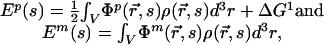
The solvation energy barrier, ΔG, is the main component to the free energy of protein insertion into the membrane (9, 10). As shown in the thermodynamic cycle in Fig. 1d, this energy has an electrostatic component, ΔG¹ + ΔG³, and a nonpolar component, ΔG^np, arising from van der Waals interactions and solvent structure effects. The electrostatic work required to move S4 from solution into the membrane–protein complex can be computed by subtracting the energy required to charge the helix in solution, -ΔG¹, from the energy required to charge the helix in the membrane–protein complex under an applied electric field, ΔG³.

We use the Poisson–Boltzmann equation to calculate the electrostatic potential:

[1]

where φ = eΦ/k_BT is the reduced electrostatic potential and Φ is the electrostatic potential; is the Debye–Hückel screening parameter, which accounts for ionic shielding; ε is the dielectric constant for each of the distinct microscopic regimes in the system; and ρ is the density of charge within the protein moiety. There are two sources of the total electrostatic potential: the explicit protein charges, ρ, and the contribution from the membrane potential. For clarity, we assume that these two fields can be linearly separated, Φ = Φ^p + Φ^m; however, this is only true for small φ. We used the superscript p to indicate the field arising from the protein charges and m to indicate the membrane potential. Both Φ^p and Φ^m are solutions to Eq. 1 with different source terms and far-field boundary conditions; however, membrane potential calculations require a modification of the sinh[φ] term so that the far-field value of Φ^m approaches V_in or V_out, the electrostatic potential of the inner or outer solution, respectively (11). For details, see Supporting Text and Fig. 6, which are published as supporting information on the PNAS web site.

Let s be a one-dimensional reaction coordinate that represents the static configuration of the S4 molecule in the protein–membrane complex. The electrostatic energy of the S4 helix is then related to the potentials by

[2]

where the ½ in the top equation comes from double counting charge–charge interactions. The total electrostatic energy of the S4 segment, relative to solution, is then E^p + E^m. For each configuration, the solvated reference energy, ΔG¹ (Fig. 1d), is determined by solving Eq. 1 for a state in which the S4 segment is surrounded by electrolyte.

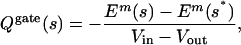
Movement of the charged residues on S4 produces a transient current that precedes the opening of the channel. When charged groups move outward across the membrane–protein complex, a cloud of counterions moves from the cytoplasm to the extracellular space. The measured gating charge is equal to the external charge transferred to the membrane capacitance to neutralize the charges that have moved. The energy required to move the charge in the external circuit under voltage clamp is Q^gate(V_in - V_out), and it is equal to the work required to move the protein charges in the membrane electric field. Thus, the observable gating charge is related to the protein's microscopic configuration:

[3]

where s* is the initial starting configuration. This result is useful because it relates the changes in the charges in solution induced by the protein charges to the energy of the protein in an external field. Formally, this result is true because the solutions to Eq. 1 for the field caused by the protein and the field caused by the membrane potential share the same Green's function. This result has been proven for the linearized form of Eq. 1 by Roux (11), and several works have applied this result to channels (12, 13). We used Eq. 3 here to make concrete connections between the models and experiment.

Computational Methods

All calculations were performed by using the program apbs 0.3.1 (14). Electrostatic solvation energies were calculated with the nonlinear equation, and the membrane potential calculations were solved in a separate step by using the linearized version. In both cases, two levels of focusing were used, and the spatial discretization at the finest level was 0.6 Å per grid point. Dielectric, charge, and ion-accessibility maps for the atomistic S4 helix were generated with apbs and then modified to add the presence of a generalized protein (Figs. 1 and 2, blue regions) embedded in a low-dielectric slab acting as a surrogate membrane (Figs. 1 and 2, pink slab). The speculative portions of the protein not modeled at the atomic level are referred to as implicit protein. See the supporting information for a more detailed description of these steps.

Fig. 2.

The central pore and a single voltage sensor corresponding to lipid-exposed (Top), translation (Middle), and rotation (Bottom) models from Fig. 1. All models show the S4 helix in the down state (red) with the top four charged groups colored yellow. (Top) The membrane–solution interface (pink) forms a plane. (Middle and Bottom) Cutaway views of the sensor show the portions of S4 surrounded by protein. (Bottom) The finger-like water vestibules on either side of S4 allow water access to the helix. Images were created with vmd (33).

All implicit protein was modeled with an intermediate dielectric value, ε, of 10.0, and the membrane was treated as ε = 2.0, which are reasonable estimates based on theoretical considerations (10, 13, 15) and experimental measurements (16). The parse parameter set was used for the S4 helix, which requires assigning ε = 2.0 to this region (17). This parameter set was calibrated by matching experimental solvation energies, which makes it a perfect match for the present study (17, 18).

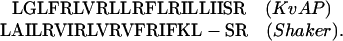
The S4 segment from Shaker was modeled onto the S4 segment from the voltage-gated potassium channel (KvAP) solo fragment by using modeller 6.2 (19) with the alignment of Jiang et al. (7):

One hundred models were generated, and the model with the lowest objective function was minimized in a vacuum with a fixed backbone by using namd 2.5 (20). The N- and C-terminal capping charges were set to zero, which did not alter the +6 net charge on the helix. All calculations involved rigid translations and rotations of this structure.

The nonpolar energy scales with the water-exposed surface area of the protein (10, 17). See the supporting information for the estimated amount of solvent-exposed surface area for each of the models at key locations along the reaction pathways.

Results

Three Models of Voltage Sensors. We have carried out calculations with three distinct geometries, each of which exemplifies a particular aspect of models from the literature.

Lipid-exposed model. MacKinnon and coworkers (8) have proposed a lipid-exposed model inspired by their structural studies of the KvAP potassium channel (7, 21). Their research suggests that the S4 helix moves a large distance (on the order of 20 Å) through membrane at the periphery of the channel. We started with the helix axis at an angle of π/3 with respect to the z axis and the helix center initially at = (-38.0,0.0,-10.0) (see Fig. 2 Top). The helix was then translated to a final position of = (-38.0,0.0,+10.0) and an angle of π/12. This is a faithful representation of the detailed model pictured in figure 5 of ref. 8. Jiang et al. (8) also propose that the S4 and S3b helices translocate together through the membrane, although the generality of this claim is debated (22). We have carried out calculations in which the electrostatic effect of the S3b helix was included by adding an intermediate-dielectric region adjacent to the S4 helix. This region is modeled as a 20-Å-long cylinder with a 7.5-Å radius and an ε of 10.0.

The dielectric map for one of these calculations is shown in Fig. 2 Top. The upper and lower membrane–solution boundaries are represented as planes. In all three models, the membrane extends from z =-15 to +15 Å. On the right of the image, part of the central pore (dark blue) is pictured penetrating the entire length of the low-dielectric membrane. The S4 helix is drawn in the down state (red), and the first four charge-carrying arginines are colored yellow. The blue S3b helix can be seen behind S4. Translation model. The earliest notions of the gating charge have centered on the idea that the S4 helix moves perpendicular to the membrane through a gating canal made up of the rest of the protein (3, 4). This concept is modeled by aligning the S4 helix with the z axis and translating it from = (-34.0,0.0,-15.0) to = (-34.0,0.0,+15.0). The surrounding protein is modeled roughly as an oblate spheroid; however, the cytoplasmic and extracellular ends are concave to allow greater solvent access to the S4 helix (see Fig. 2 Top). This geometry can easily be seen from the cutaway picture of the voltage sensor in Fig. 2 Middle. The helix is centered at z = -10.0 Å, which makes the two uppermost arginines (R362 and R365) inaccessible to solution in accord with studies carried out on Shaker in the down state (23). The inner and outer solutions are separated by a thin septum of ≈5 Å, which is consistent with experiment (6, 23). The central pore is pictured to the right of the sensor. The membrane boundaries extend from just below the top of the sensor to just above its bottom, but they were omitted for clarity.

Rotation model. It has also been suggested that the gating motion is dominated by a rotation of the S4 helix about its axis (24). In this model, the charged residues are transported from an inner vestibule to an outer vestibule moving 3–4 charges across the membrane electric field while the helix center of mass remains largely fixed. Note that this hypothetical vestibule around the voltage sensor is not the same as the water vestibule seen in ion channel structures (25). The gating vestibules are modeled by quadratic conic sections with opening diameters of 10 Å, and later by a wider opening of 21 Å. The use of a quadratic function, compared to a lower power polynomial, allows for more significant penetration of the solvent into the sensor. The S4 center is positioned at the sensor center = (-34.0,0.0,0.0), and both vestibules and the helix are tilted at an angle of π/12 with respect to the membrane normal.

Fig. 2 Bottom shows the dielectric map for the rotation model with the S4 helix in the down state. The cutaway view of the sensor domain shows that the four principal charge-carrying arginines face the cytoplasmic vestibule. The larger central pore is positioned behind the voltage sensor, and the membrane boundaries, which are not pictured, are 2 Å smaller than the vertical extent of the voltage sensor.

Solvation Barriers: Exposing S4 to Lipid Requires Considerable Energy. Electrostatic work, E^p, is required to move the S4 segment from aqueous solution into a low-dielectric, solvent-inaccessible space. Microscopically, this action corresponds to displacing polar water molecules, initially in close contact with the protein surface and replacing them by less polar molecules. Therefore, the charged arginine and lysine groups require the most work to move through the membrane–solution interface. The electrostatic solvation energy for each model as it undergoes its respective gating motion is plotted in the left column of Fig. 3, and the right column shows the corresponding gating charge transferred from the cytoplasm to the extracellular solution. The translation and rotation models require comparable electrostatic work, E^p ≈ 50 k_BT. In marked contrast, the lipid-exposed model requires 280–450 k_BT of electrostatic work to move the S4 segment from solution into lipid. There are two reasons for the large energy difference between the models. First, the lipid-exposed model has little direct contact between the S4 helix and solvent, whereas the small septa separating the inner and outer solutions in the rotation and translation models maximize the water access to S4 at all points along the reaction pathway. This latter geometry is supported by the observation that particular channel mutations allow protons to flow through the voltage sensor (6). Second, charged residues on S4 contact protein, not lipid, in the translation and rotation models. Proteins are generally much more polar than lipids; therefore, the protein environment is better suited for substituting charge contacts lost between S4 and water molecules. We therefore considered the effect of including the S3b helix adjacent to the non-arginine face of S4 in the lipid-exposed model. S3b was represented by a slab of intermediate, protein-like dielectric, which lowered the electrostatic solvation energy by ≈30 k_BT (Fig. 3a, dashed curve). For typical biological energy scales, this decrease is notable; however, given the large electrostatic component of the solvation barrier, it may be insignificant.

Fig. 3.

Total electrostatic solvation energy of the S4 segment and gating charge movement for lipid-exposed (a), translation (b), and rotation (c) models. (Left) Plots of the solvation energy. (Right) Plots of the total gating charge along the reaction pathway. The dashed curve represents the effect of the S3b helix on the lipid-exposed model. The solvation energy profile for the rotation model is rugged because of the complicated interfacial geometry.

The solvation energy is incomplete without considering the nonpolar or hydrophobic effect, which stabilizes solute molecules in the membrane. This stabilization is proportional to the buried surface area, which, for the translation and rotation models, is nearly constant throughout the gating transition. From estimates of the buried area, we predict that S4 is stabilized by approximately -30 k_BT and -60 k_BT for these two models, respectively. When combined with the electrostatic energies in Fig. 3, the total solvation energy is centered on zero, making the translation and rotation models physically reasonable. Most impressively, the lipid-exposed model is stabilized by ΔG^np ≈ -120 k_BT, because nearly the entire 2,600-Ų surface of S4 is buried. Accounting for the solvent exposed surface area in the initial and final states, the total solvation barrier for the lipid-exposed model is 200–320 k_BT or 180–290 k_BT if the electrostatic effect of S3b is included. Given such large energies, it is difficult to imagine that the rest of the channel could be stable enough to adopt the sensor configurations of the lipid-exposed model without denaturing; however, this is speculative.

Gating Charge Transfer: A Large Gating Charge Mandates Outward S4 Motion. Each subunit produces a gating charge of 3.0–3.4 electron charge units during gating (1, 2). Gating charge transfers of equal or greater value are required for a model to be physically plausible. Both the lipid-exposed model and the translation model produce gating charge values between 3 and 4 charge units. This value is quite robust, owing to the large displacement of the S4 segment from the cytoplasm to the extracellular solution, which ensures that in the down state nearly all induced charge is in the inner solution and in the up state induced charge is primarily in the outer space. As the rotation model undergoes a π rotation from π to 2π, 0.6 charge units are moved across the interface, which is 6- to 7-fold smaller than observed. This shortcoming is due to the geometry of the sensor and the helical placement of the charged groups on S4 (Fig. 2, yellow stripe).

Fig. 4 shows cross sections of the voltage sensor through the center of the S4 segment viewed from the central pore. The membrane potential isocontours are plotted overtop of this geometry. Fig. 4a corresponds to the model used in Fig. 3c, and an alternative geometry with a 21-Å-wide vestibule is pictured in Fig. 4b. The uniformity of the potential contour lines across the vestibules shows the first major shortcoming of the pure rotation model. In Fig. 4a, there is a 60% drop of the field from bulk solution to the bottom of the vestibule. Therefore, charged residues at this deeper position only traverse a fraction of the membrane electric field as they move from the inner to the outer solution. The vestibules support an electric field, despite the large dielectric value of water, because the field is clamped by the low-dielectric environment of the membrane, and the small horizontal extent of the vestibule allows little variation in the potential from one side to the other. Increasing the size of the vestibule in panel b decreases the field attenuated across its length to 40%. This focuses the field across the S4 segment and increases the fraction of the external field through which the S4 charges pass as the helix rotates. A pure rotation within the larger vestibule nearly doubles the gating charge from 0.6 to 1.1 charge units. However, this value is still 3-fold smaller than experimentally measured, despite the exceedingly large vestibule. Because the charged residues of S4 are not perfectly aligned, as the helix rotates into the up state, the bottom charges begin to exit the extracellular vestibule as the top charges enter the vestibule. Movement of charges back toward the cytoplasmic space reduces the charge transferred to the outer solution. In Fig. 4 c and d, a modified gating motion is proposed in which the helix first tips or rocks between vestibules while rotating and then undergoes a 7.5-Å vertical translation. The sensor geometry is as in Fig. 4b, but the modified motion produces a more physically realistic charge transfer of 2.2 charge units. Such a motion has been suggested by Bezanilla (24), but it is an open question whether the vestibules and the proposed translation in his proposed molecular model are large enough to produce the desired gating charge.

Fig. 4.

Membrane potential profile across the rotation model sensor. The system is divided into three distinct regions: water (white, ε = 80), voltage sensor (light gray, ε = 10), explicit S4 helix, and membrane (dark gray, ε = 2). The electrostatic potential was generated by solving Eq. 1 in the absence of protein charges with V_in =-2.0 k_BT (approximately -51.4 mV). Equipotential lines are superimposed over the sensor geometry every 5 mV. (a) The standard rotation model. (b) The mouth of the vestibule has been increased to 21 Å. (c and d) Two configurations of a modified gating movement in which S4 starts in the down state (red), rotates by π radians, tips across the septum separating the inner and outer vestibules, and is translated into the up state (green).

Membrane Potential and Transition Rates: The Lipid-Exposed Transition Prohibits Channel Activation. The influence of the membrane potential on S4 is determined from the gating charge curves in Fig. 3. At negative potentials, the field interaction biases the energy levels so that the down and up states are reversed from their resting values. The amount by which the down state is shifted with respect to the up state is ΔE = Q^gate·(V_in - V_out). From the total solvation energy, all three models predict that the up state is stabilized in zero field (by -20 k_BT for the lipid-exposed model and -10 k_BT for the translation and rotation models), which is consistent with the experiment. At -75 mV, the field stabilized the down state by 3.4·-75 mV·1 k_BT/25 mV = -10 k_BT, and experimentally S4 adopts the down state. This energy is comparable to the solvation energy differences predicted by the translation and rotation models, making it possible for the membrane potential to switch S4 to the down state. However, because Q^gate is 0.6 for the rotation model, the gating energy is only 2 k_BT, which is too small to close the channel. This small gating energy highlights the need for a modified reaction pathway as in Fig. 4 c and d. Even though Q^gate is large for the lipid-exposed model, the energy of the down state is still 10 k_BT higher than the energy of the up state at -75 mV. This difference is close and may be remedied by the influence of other charged residues or changes to the initial and final configurations.

Voltage-gated potassium channels open on the millisecond time scale. Before channels can open, the S4 segment must surmount the solvation barrier. The translation model presents a barrier on the order of 10 k_BT, whereas it is ≈100 k_BT for the lipid-exposed model. The energy profile of the rotation model is complicated, so we forgo a discussion of its activation kinetics. From Kramers' reaction rate theory, the activation time is proportional to the exponentiated barrier energy, ΔG_act, divided by the diffusion coefficient of the molecule: τ ∝ [1/D]exp(ΔG_act) (see the supporting information for a more complete discussion) (26). The S4 diffusion coefficient along the respective reaction coordinates for each of these models is not known; however, we can make a rough estimate based on the lateral diffusion coefficient of gramicidin C in lipid bilayer, D = 3 × 10⁸Ų/s (27). By using this calculation, we arrive at millisecond activation times for the translation model. The lack of large barriers in the rotation model suggests an activation time comparable to this value. Meanwhile, the lipid-exposed model activates 10³⁸ times more slowly. Such long times are inconsistent with experiment, bringing to bear one of the strongest arguments against the lipid-exposed model as presented here.

Revisiting E^p Calculations: Modest Lipid Exposure Is Permissible. Biotin-avidin experiments on KvAP have been used to suggest that the S4 helix has extensive contact with lipid (8); however, alanine-scanning mutagenesis on both Shaker and EAG has been used to support a more conservative interaction between just the hydrophobic face of S4 and the membrane (28, 29). With regard to gating, diffusion through fluid lipid molecules may be faster than diffusion through a gating canal composed entirely of protein, which highlights an attractive property of the lipid-exposed model and suggests that we may have overestimated the diffusion coefficient of the translation model above. However, as we have seen, there is a large energy penalty associated with surrounding S4 by lipid. We examined one final model calculation to determine the energetic cost associated with introducing limited exposure of S4 to the membrane. We started by wrapping the entire S4 helix in an intermediate-dielectric environment of ε = 10.0 with a radius of 22.0 Å and then exposed the helix to a wedge of lipid (see Fig. 5). The fully wrapped sensor geometry is similar to the one used in the translation model, but the implicit protein forms a right cylinder centered on S4. The electrostatic energy required to expose the helix to a 3π/8 solid angle of lipid, as pictured in Fig. 5 Inset,is ≈50 k_BT (Fig. 5, solid curve). This configuration results in a dramatic reduction in energy when compared with the previous calculations on the lipid-exposed model. For lesser degrees of exposure, the energetic destabilization is on the order of 20–25 k_BT, which may be reasonable for a membrane protein designed to perform such a dynamic task. We also carried out the same calculations, but with the hydrophobic face of the helix exposed to the lipid environment (Fig. 5, dashed curve). Exposing a π/2 swath of helix to lipid requires only 10 k_BT of energy. Therefore, the helix can have significant membrane exposure, with very minor increases in energy, as long as the charge-carrying residues remain buried in protein. Interestingly, electron paramagnetic resonance experiments recently performed on the KvAP channel appear to corroborate this last scenario (30).

Fig. 5.

Electrostatic energy required to expose S4 to membrane. The S4 segment (center of Inset) was wrapped in an intermediate-dielectric region (ε = 10.0) and then exposed to low-dielectric wedges (ε = 2.0). The solid angle of the wedge was increased from 0 to π/2, and the electrostatic energy with respect to the nonexposed state was plotted for the charge carrying side (solid curve) or the hydrophobic side (dashed curve) facing the wedge. (Inset) Top-down view of sensor configurations for solid angles 3π/8 (explicit) and π/2 (schematic). The angular extent of the lipid wedge is indicated by curved arrows. The explicit diagram shows the red, 2.01 isocontour of the dielectric map corresponding to the membrane and S4 helix. The surrounding sensor and central pore are black.

Discussion

We have quantitatively evaluated three different modes of voltage sensing in voltage-gated potassium channels by calculating the work required to move the S4 helix through the membrane–solution interface and the interaction energy of the helix with the transmembrane electric field. This latter calculation allowed us to compute theoretical gating charge values for each hypothetical gating motion and to compare them with experimental values. We showed that the attenuation of the electric field across water-filled crevices surrounding the S4 segment severely limits the charge that can be transferred by a pure rotation. Increasing the size of the water vestibules partly ameliorates this problem, but tipping and translating the S4 segment in the sensor is required to produce moderate gating charge values. Both the lipid-exposed model and the pure translation model produce large gating currents because of the motion of all of the charged groups a significant distance perpendicular to the membrane potential isocontours.

The pure rotation and translation models both have modest solvation energies on the order of 50 k_BT because of the partial solvation of S4 in the sensor and the intermediate-dielectric properties of the sensor domain. However, the lipid-exposed model buries the charged groups on S4 in the low-dielectric membrane, where they lose contact with water. This feature leads to solvation energies on the order of hundreds of k_BT and an energy barrier for activation of ≈100 k_BT. By using reasonable values for the diffusion coefficient of the S4 segment, we showed that the translation model activates on the millisecond time scale but that the lipid-exposed model activates many orders of magnitude more slowly. This latter result is incompatible with the observed kinetics of voltage-gated channels.

Acidic groups in segments S2 and S3 have been shown to influence the gating process (1, 31). Earlier theoretical calculations showed that the interactions between S4 and these charges could account for voltage shifts in gating charge curves from mutant channels (13), but we have not considered their effect here. Predicted gating charge values depend only on sensor geometry and are therefore insensitive to this omission. The discussion of the lipid-exposed model will also not be affected, because salt-bridge energies are much smaller than the calculated solvation energies. However, the energetics of gating for the translation and rotation models will be substantially modified by the inclusion of additional charges. Subsequent calculations must include their effect to explain gating charge curves in detail.

The conformational changes of voltage-gated channels are driven by membrane potential, and because the voltage sensor is highly charged, the free energy of gating is most likely dominated by electrostatics. Therefore, Poisson–Boltzmann theory is a good first approach to quantifying the physics of voltage-sensing. The flexibility with which detailed geometric shapes can be incorporated into the apbs solver is well matched to the level of structural detail available for this class of channels. Our approach has allowed us to analyze many distinct hypothetical sensor geometries and gating motions with very little computational effort, thus providing a fast method for testing and honing different models. We used a parameter set that has been optimized to reproduce experimentally measured solvation energies (17, 18), so we can expect that the values calculated herein are quite accurate. However, we assumed that the lipids pack regularly around the voltage sensor, and we ignored the packing energetics of the bilayer around the channel. It is conceivable that the lipid and water organization around the S4 helix is drastically different from that assumed for the lipid-exposed model, in which case, the predicted energies would be subject to modification. Detailed investigations into charged groups crossing lipid bilayers will be required to properly address this issue. Meanwhile, our approach can be used to examine the influence of the membrane and the membrane potential on other channels and transporters, such as the MscS voltage-modulated and mechanosensitive channel (32). Interestingly, this structure reveals arginine groups, hypothesized to be voltage-sensing, poised at what would be the membrane–protein interface.

In conclusion, modeling shows that a pure rotation of the S4 helix fails to produce experimentally measured gating charge values. In contrast, the translation and lipid-exposed models do not suffer from this shortcoming. When the S4 segment is directly exposed to bilayer, a prohibitively large solvation barrier is created that prevents channel activation. However, the channel incurs only modest destabilization if the exposure of S4 to the membrane is limited.

References

- 1.Seoh, S. A., Sigg, D., Papazian, D. M. & Bezanilla, F. (1996) Neuron 16, 1159–1167. [DOI] [PubMed] [Google Scholar]
- 2.Aggarwal, S. K. & MacKinnon, R. (1996) Neuron 16, 1169–1177. [DOI] [PubMed] [Google Scholar]
- 3.Catterall, W. A. (1986) Annu. Rev. Biochem. 55, 953–985. [DOI] [PubMed] [Google Scholar]
- 4.Guy, H. R. & Seetharamulu, P. (1986) Proc. Natl. Acad. Sci. USA 83, 508–512. [DOI] [PMC free article] [PubMed] [Google Scholar]
- 5.Cha, A., Snyder, G. E., Selvin, P. R. & Bezanilla, F. (1999) Nature 402, 809–813. [DOI] [PubMed] [Google Scholar]
- 6.Starace, D. M. & Bezanilla, F. (2004) Nature 427, 548–553. [DOI] [PubMed] [Google Scholar]
- 7.Jiang, Y., Lee, A., Chen, J., Ruta, V., Cadene, M., Chait, B. T. & MacKinnon, R. (2003) Nature 423, 33–41. [DOI] [PubMed] [Google Scholar]
- 8.Jiang, Y., Ruta, V., Chen, J., Lee, A. & MacKinnon, R. (2003) Nature 423, 42–48. [DOI] [PubMed] [Google Scholar]
- 9.Jacobs, R. E. and White, S. H. (1989) Biochemistry 28, 3421–3437. [DOI] [PubMed] [Google Scholar]
- 10.Ben-Tal, N., Ben-Shaul, A., Nicholls, A. & Honig, B. (1996) Biophys. J. 70, 1803–1812. [DOI] [PMC free article] [PubMed] [Google Scholar]
- 11.Roux, B. (1997) Biophys. J. 73, 2980–2989. [DOI] [PMC free article] [PubMed] [Google Scholar]
- 12.Islas, I. D. & Sigworth, F. J. (2001) J. Gen. Physiol. 117, 69–89. [DOI] [PMC free article] [PubMed] [Google Scholar]
- 13.Lecar, H., Larsson, H. P. & Grabe, M. (2003) Biophys. J. 85, 2854–2864. [DOI] [PMC free article] [PubMed] [Google Scholar]
- 14.Baker, N., Sept, D., Joseph, S., Holst, M. J. & McCammom, J. A. (2001) Proc. Natl. Acad. Sci. USA 98, 10037–10041. [DOI] [PMC free article] [PubMed] [Google Scholar]
- 15.Warshel, A. & Papazian, A. (1998) Curr. Opin. Struct. Biol. 8, 211–217. [DOI] [PubMed] [Google Scholar]
- 16.Cohen, B. E., McAnaney, T. B., Park, E. S., Jan, Y. N., Boxer, S. G. & Jan, L. Y. (2002) Science 296, 1700–1703. [DOI] [PubMed] [Google Scholar]
- 17.Sitkoff, D., Sharp, K. A. & Honig, B. (1994) J. Phys. Chem. 98, 1978–1988. [Google Scholar]
- 18.Wolfenden, R., Andersson, L., Cullis, P. M. & Southgate, C. C. (1981) Biochemistry 20, 849–855. [DOI] [PubMed] [Google Scholar]
- 19.Sali, A. & Blundell, T. L. (1993) J. Mol. Biol. 234, 779–815. [DOI] [PubMed] [Google Scholar]
- 20.Kale, L., Skeel, R., Bhandarkar, M., Brunner, R., Gursoy, A., Krawetz, N., Phillips, J., Shinozaki, A., Varadarajan, K. & Schulten, K. (1999) J. Comp. Phys. 151, 283–312. [Google Scholar]
- 21.Jiang, Q., Wang, D. & MacKinnon, R. (2004) Nature 430, 806–810. [DOI] [PubMed] [Google Scholar]
- 22.Cohen, B. E., Grabe, M. & Jan, L. Y. (2003) Neuron 39, 395–400. [DOI] [PubMed] [Google Scholar]
- 23.Larsson, H. P., Baker, O. S., Dhillon, D. S. & Isacoff, E. Y. (1996) Neuron 16, 387–397. [DOI] [PubMed] [Google Scholar]
- 24.Bezanilla, F. (2002) J. Gen. Physiol. 120, 465–473. [DOI] [PMC free article] [PubMed] [Google Scholar]
- 25.Doyle, D., Morais Cabral, J., Pfuetzner, R. A., Kou, A., Gulbis, J. M., Cohen, S. L., Chait, B. T. & MacKinnon, R. (1998) Science 280, 69–77. [DOI] [PubMed] [Google Scholar]
- 26.Risken, H. (1989) The Fokker–Planck Equation (Springer, New York).
- 27.Tank, D. W., Wu, E. S., Meers, P. R. & Webb, W. W. (1982) Biophys. J. 40, 129–135. [DOI] [PMC free article] [PubMed] [Google Scholar]
- 28.Li-Smerin, Y., Hackos, D. H. & Swartz, K. J. (2000) Neuron 25, 411–423. [DOI] [PubMed] [Google Scholar]
- 29.Schönherr, R., Mannuzzu, L. M., Isacoff, E. Y. & Heinemann, S. H. (2002) Neuron 35, 935–949. [DOI] [PubMed] [Google Scholar]
- 30.Cuello, L. G., Cortes, D. M. & Perozo, E. (2004) Science 306, 491–495. [DOI] [PubMed] [Google Scholar]
- 31.Tiwari-Woodruff, S. K., Schulteis, C. T., Mock, A. F. & Papazian, D. M. (2002) Biophys. J. 296, 1700–1703. [DOI] [PMC free article] [PubMed] [Google Scholar]
- 32.Bass, R. B., Strop, P., Barclay, M. & Rees, D. C. (2002) Science 298, 1582–1587. [DOI] [PubMed] [Google Scholar]
- 33.Humphrey, W., Dalke, A. & Schulten, K. (1996) J. Mol. Graphics 1, 33–38. [DOI] [PubMed] [Google Scholar]
Associated Data
This section collects any data citations, data availability statements, or supplementary materials included in this article.