Social monogamy in wild owl monkeys (Aotus azarae) of Argentina: the potential influences of resource distribution and ranging patterns

Abstract

Using published and new data from a population of monogamous owl monkeys in the Argentinean Chaco, I examine the hypothesis that social monogamy is a default social system imposed upon males because the spatial and/or temporal distribution of resources and females makes it difficult for a single male to defend access to more than one mate. First, I examine a set of predictions on ranging patterns, use of space, and population density. This first section is followed by a second one considering predictions related to the abundance and distribution of food. Finally, I conclude with a section attempting to link the ranging and ecological data to demographic and life-history parameters as proxies for reproductive success. In support of the hypothesis, owl monkey species do live at densities (7 to 64 ind/km²) that are predicted for monogamous species, but groups occupy home ranges and core areas that vary substantially in size, with pronounced overlap of home ranges, but not of core areas. There are strong indications that the availability of food sources in the core areas during the dry season may be of substantial importance for regulating social monogamy in owl monkeys. Finally, none of the proxies for the success of groups were strongly related to the size of the home range or core area. The results I present do not support conclusively any single explanation for the evolution of social monogamy in owl monkeys, but they help us to better understand how it may function. Moreover, the absence of conclusive answers linking ranging, ecology, and reproductive success with the evolution of social monogamy in primates, offer renewed motivation for continuing to explore the evolution of monogamy in owl monkeys.

Introduction

“The hypothesis, broadly stated, that mating systems are an outcome of the distribution of resources has a seductive charm about it, so much so that we tend to fit findings into its framework rather than attempt to falsify it. To a large degree, I have been guilty of this sin in this essay.”

[Barlow, 1988: 69]

Although social monogamy, defined as a system where an adult individual has only one social partner of the opposite sex at a given time (Table 1), is most common among birds, it also occurs in invertebrates, fish, amphibians, reptiles, and mammals [Möller, 2003]. Among mammals, social monogamy has been argued to be most common among rodents, canids, and primates [Lukas and Clutton-Brock, 2013]. In the case of primates, there is considerable variation in the number of socially monogamous species reported over the years [Fuentes, 1999; Lukas and Clutton-Brock, 2013; Opie et al., 2013]. This variation is likely influenced by the numerous ways in which various authors have defined and characterized monogamy, pair-bonding, and pair-living [Kappeler, 2014; Tecot, this volume]. For example, the callitrichines were classified as “socially monogamous” in a recent analysis based principally on information obtain through studies of captive individuals [Opie et al., 2013], even when numerous field studies suggest that monogamy is not the common or modal breeding system for them [Garber et al., this volume].

Table 1. Definitions.

Social Monogamy	An adult individual has only one social adult partner of the opposite sex at a given time (Huck et al. 2013). It is necessary to note that there have been studies considering as socially monogamous species where “the majority of breeding females (>50%) share a home-range for more than one year with one male, but no other conspecific breeders” [Lukas and Clutton-Brock, 2013 Supplementary Materials].
Pair-living	Frequently used in the primate literature in the same manner as “social monogamy”
Genetic Monogamy	The only adult male and only adult female in a socially monogamous group sire the offspring in the group. The extreme form of genetic monogamy implies that there is zero extra-pair paternity, with 100% of the offspring in the group assigned to the resident adult male [Huck et al. 2014]. In some analyses an arbitrary cutoff of percentage of offspring sired by the pair may be considered.
Pair-bond	The term is used to refer to two reproducing adults who have a strong emotional attachment as reflected in their affiliative interactions, proximity, distress upon separation from the pairmate, and reduced anxiety following reunion with the pairmate [Mason and Mendoza, 1998]. In field primatology, the term is regularly used for describing socially monogamous or pair living primates even when no evidence exists of an enduring, stable, emotional attachment.

In the early theoretical approaches, hypotheses explaining the evolution and maintenance of monogamy tended to fall into one of two classes. Some suggested that monogamy was a default social system imposed upon males when either the spatial or temporal distribution of females made it difficult for single males to simultaneously defend access to more than one mate [Emlen and Oring, 1977; Rutberg, 1983; van Schaik and van Hoof, 1983]. Other models proposed that monogamy evolved in response to the need for obligate biparental care in order to successfully rear offspring [Kleiman, 1977; Wittenberger and Tilson, 1980; Woodroffe and Vincent, 1994]. Over the years, there has been growing consensus that biparental care is unlikely to be a driving factor for the evolution of monogamy and instead may evolve, under certain circumstances such as reduced father uncertainty, once social monogamy exists [Brotherton and Komers, 2003; Dunbar, 1995; Komers, 1996; Komers and Brotherton, 1997; Lukas and Clutton-Brock, 2013; Lukas and Huchard, 2014; Opie et al., 2013].

I explore the hypothesis that social monogamy is imposed upon males because the spatial and/or temporal distribution of resources and females make it difficult for them to defend access to more than one mate. This hypothesis, which has received strong support from mammal-wide analyses of social monogamy [Brotherton and Komers, 2003; Dobson et al., 2010; Lukas and Clutton-Brock, 2014; Lukas and Clutton-Brock, 2013], proposes that females are distributed in space matching the availability of food. Under certain ecological conditions, possibly associated with a habitat that only provides relatively scarce food, females space themselves individually, and with relatively little overlap among ranges to minimize competition over food. The resulting size of female home ranges precludes males from monopolizing more than one female. It has been challenging to find a primate system to test these ideas since most primates use relatively large ranges in forests with very diverse floristic composition, conditions that make it hard to thoroughly evaluate the distribution of resources in the ranges of several groups.

A population of owl monkeys in the Argentinean Chaco is well-suited for testing predictions derived from this hypothesis given their relatively small ranges and the low diversity of plant species they consume [Arditi, 1992; Giménez and Fernandez-Duque, 2003; Giménez, 2004]. A typical group includes only one pair of reproducing adults, one infant, one or two juveniles and sometimes a subadult [Fernandez-Duque et al., 2001; Huck et al., 2011]. The reproducing pair has a close socio-spatial relationship and shows both social and genetic monogamy [Fernandez-Duque and Huck, 2013; Huck et al., 2014a; Huck and Fernandez-Duque, 2012]. Females produce one offspring per year; twinning is extremely rare in owl monkeys both in the wild and captivity [Huck et al., 2014b]. Reproduction is highly seasonal with 80% of births occurring during October-November [Fernandez-Duque et al., 2002].

A comprehensive evaluation of the female distribution hypothesis requires the quantitative characterization of the temporal and spatial distribution of resources and the ranging patterns of males and females. This is necessary since it is based on assumptions concerning a direct relationship between ranging and food distribution that limits the ability of males to monopolize more than one female. For example, if one found that the size of the home ranges of some owl monkey groups were twice as large as others, this would indicate that males who occupy these larger ranges could potentially maintain access over the range of two or more females inhabiting “small” ranges. In other words, if one showed that adult males have the ranging capability to monitor more than one female range in a monogamous population, one may need to explore other factors limiting the monopolization of females. In addition to the size of female ranges per se, the extent of home range overlap needs to be considered since it will influence the effective area over which a male needs to range. At one theoretical extreme, if two females exhibit complete overlap of their ranges, then a male could monopolize both of them if his ability to do so is only constrained by the area over which they range. On the other hand, two adjacent female ranges that do not overlap, would double the area over which a male would need to control, especially if females are receptive during the same period of the year. Under a null model of ranging patterns and use of space being equal across groups, the hypothesis proposes that the food base in each of those ranges is similar, and therefore only sufficient to support one female and one male. Finally, the ultimate test of an evolutionary hypothesis that proposes a relationship between ranging patterns, use of space, food availability and mating system must include an examination of the actual reproductive success of groups under different ecological conditions. If monogamous groups are occupying similar areas with similar resources, one expects to find similar reproductive success for all groups. Exploring a number of life-history and demographic variables (e.g. infant production, mortality, age at dispersal) can provide reasonable proxies for assessing the “success” of groups.

Using published and unpublished information gathered by the Owl Monkey Project (OMP) of Argentina, I test 10 predictions derived from the hypothesis that social monogamy in owl monkeys is primarily explained by the temporal and spatial distribution of resources, which in turn determines the distribution of females and males (Table 2). I have organized the predictions in three groups; the first set of predictions examines ranging patterns, use of space and population density. The second considers evidence based on the abundance and distribution of food, and the last one links the ranging and food data to demographic and life-history data as proxies of reproductive success. For each set of predictions I present the available data from the OMP and then consider it in the context of similar data from other monogamous primate/mammal taxa, at all times bearing in mind the limitations inherent to the correlational nature of data generated in field studies [Janson, 2012].

Table 2. Predictions.

Ranging patterns, use of space and population density	P1	Given the relatively small spatial variation in the gallery forest structure and composition (Placci, 1995;Van der Heide et al, 2012) there will be a relatively even spatial distribution of food If food is more or less evenly distributed in space, the size of the space regularly used by groups will not vary much among groups.
	P2	Given the lower densities found among monogamous species (Lukas and Clutton-Brock, 2013), owl monkey species will be found at relatively low densities across their distribution.
	P3	Given the relatively smaller overlap of ranges in monogamous mammals (Lukas and Clutton-Brock, 2013), the overlap of owl monkey ranges should be relatively small.
Abundance, temporal and spatial distribution of food	P4	Given that some home ranges are larger than others, larger territories will be “poorer” in quality than smaller ones, and therefore all territories will provide similar amounts of food.
	P5	Given the seasonal nature of the area (Placci, 1995; Fernandez-Duque et al. 2002), owl monkey home ranges will be relatively similar in the temporal distribution and abundance of trees providing food sources.
	P6	If the dry season acts as a bottleneck, owl monkeys will occupy areas that provide enough food during the harshest times. It is then predicted that there will be no marked differences among home ranges in fruit load during the dry season.
Group demography and life-history traits	P7	Assuming that the number of infants produced will be intimately related to the nutritional status of females, which will be related to available food, the number of infants produced in different home ranges will not show much variation.
	P8	Assuming that access to food resources will be intimately linked to the health and survival of dependent infants and growing juveniles, there will be no marked differences in infant and juvenile mortality among home ranges.
	P9	If home ranges had similar amounts of resources, group sizes will be similar.
	P10	Assuming that the age when individuals disperse from their natal groups may be partially influenced by competition for resources within the group, there will be no differences among groups in the mean age at dispersal.

Methods

All research described here was endorsed by the National Wildlife Directorate in Argentina and approved by the ethics committees (IACUC) of the Zoological Society of San Diego (2000-2005) and of the University of Pennsylvania (2006-2012). The research adhered to the American Society of Primatologists' principles for the ethical treatment of primates.

Area of study

Our research in the Owl Monkey Project takes place in the Argentinean Gran Chaco (Figure 1). The South American Gran Chaco occupies 1,000,000 km² of Bolivia, Brazil, Argentina and Paraguay and is the second largest biome in South America. Since 1996 we have been working in the gallery forests along the many rivers that cross the region in the Province of Formosa [Brown et al., 1993; Juárez, 2012; Juárez et al., 2012; Placci, 1995]. All of the research summarized here has been done within the approximately 5,000 hectares of gallery forest that grows along the Pilagá and Guaycolec rivers in the 25,000 ha Guaycolec Ranch.

Figure 1.

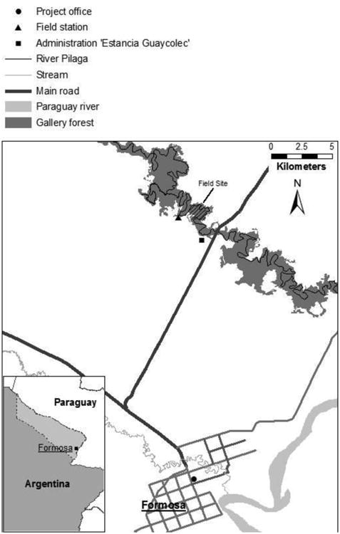
Location of the study area in the Guaycolec Ranch, Formosa Province, Argentina.

A section of approximately 1,500 ha of gallery forest was established as the Reserva Mirikiná (Owl Monkey Reserve) in 1996. These gallery forests have relatively small spatial variation in structure and composition [Placci, 1995; van der Heide et al., 2012]. The ecological, demographic and behavioral data presented here were collected from groups ranging primarily within the reserve. A system of intersecting transects at 100 m intervals covers approximately 300 ha of forest where all of the ecological and ranging data, and demographic data from 20 groups were collected. The remaining seven groups from which demographic data were collected are found in the same forest type between 1-3km away from the transect system.

The mean annual precipitation in the Guaycolec ranch was 1,418 mm (± 337, 1977-2013, OMP Database). Monthly mean rainfall varies significantly during the year, with two rain peaks in April (197 ± 166 mm) and November (186 ± 122 mm), with the lowest mean (51 ± 51 mm) for the period of June through August. Monthly mean temperatures are lowest between May and August (16-18 °C) and highest between October and March (23-27 °C). Extreme low and high temperatures are frequent. Daily minimum temperatures <10°C occur frequently between April and September; whereas maximum daily temperatures >33°C are common between September and March [Fernandez-Duque et al., 2002].

Ecological data

A complete survey of all trees and lianas (DBH > 10cm) in 16.25 ha of gallery forest identified 7485 individuals belonging to 65 species, 59 plant genera, and 30 plant families. Most species were trees (n=43), some were small trees (treelets) or shrubs (n=14), a few were lianas (n=5), one was a palm, one was a cactus, and one was a hemiepiphyte. There are four main types of habitats within the gallery forests: flooded, high and low albardón (a Spanish word used to refer to riverine forests situated on lateral, sandy-silt deposits from the riverbeds) and Austro-Brazilian transitional forest [Fernandez-Duque, 2003; Neiff, 2005; Placci, 1995; van der Heide et al., 2012]. The flooded forest, found along a 20-100 m wide belt along the margins of the Pilagá River, is relatively open and dominated by a few tree species of low stature only found in this type of forest. The other three forest types are more floristically diverse, contain taller trees (± 15 m with emergent trees of 25 m), and constitute a botanical gradient of decreasing altitude, utilizable soil layer depth, and water holding capacity from the river to the savannah. Certain species exclusively or preferentially grow on specific parts of the gradient and typify the three forest types accordingly.

The data on forest composition and structure were gathered with two different sampling designs. In 1997 we established 30 10×50m plots randomly within 30 ha of forest corresponding approximately to the home ranges of six owl monkey groups [Fernandez-Duque et al., 2002]. Between 2005-2008 we collected ecological data from 7485 individual trees distributed in the 16.25 hectares that roughly corresponded to the home ranges of four of those six groups [van der Heide et al., 2012]. We measured the DBH, identified the species, and tagged the stem of all trees and lianas with a diameter at breast height ≥ 10 cm (DBH: 1.3 m above ground). We mapped, with reference to the transect system, all trees with a DBH ≥ 30 cm and all trees belonging to 48 species reported to be important in the diet of owl monkeys at a site 10 km upstream from our area of study [Arditi, 1992] and known to be regularly consumed by owl monkeys at our site.

The forest shows a strong seasonal pattern in the production of leaves, flowers and fruits [van der Heide et al., 2012]. This finding, which matches earlier reports [Fernandez-Duque et al., 2002; Placci, 1995] is based on monthly data on the timing, duration and intensity of tree and liana phenophases of individuals located in the 30 50×10 m plots previously mentioned. During 1998-1999 the monthly sample included all 1,000 trees with DBH > 10cm [Fernandez-Duque et al., 2002]. No monthly phenological data were collected during 2000-2002. Beginning in 2003, we selected a subset of the 1,000 trees in those plots for monthly phenological monitoring. During 2003-2008, the subset consisted of 272 trees and since 2009 it was increased to 441 trees. Since 2003 the subset of monthly monitored trees has always included 5-10 individuals of each of the 48 species that have been identified as regular food items in the owl monkey's diet [van der Heide et al., 2012]. Since 2003 the phenological data have always been collected similarly; we collect categorical data recording the percentage of the tree crown containing a particular phenophase (leaves: 0-1, 1-5, 5-10, 10-25, 25-50, 50-75, 75-100%; flower buds and flowers: 0-25, 25-50, 50-75, 75-100%) and we calculate fruit loads of immature, intermediate, mature, overmature fruits, and fruits of unknown maturity by counting all fruits in a visible portion of the crown and multiplying that count by the total number of even-sized portions with fruits in the crown. During July-August of 2008 and 2009 we assessed, in more detail, food availability during the dry season [Fernandez-Duque and van der Heide, 2013]. We collected, twice a month, phenological data from 894 individuals belonging to the six species (Chrysophyllum gonocarpum, Guazuma ulmifolia, Syagrus romanzoffiana, Tabebuia heptaphylla, Enterolobium contortisiliquum, Ficus spp.) that provide most (ca. > 60%, Table 1 in Fernandez-Duque et al. 2013) of the dry season food resources. This more intense sampling was done within the 16.25 ha that completely encompassed the four owl monkey home ranges mentioned above.

Demographic and ranging data

The owl monkey population in the gallery forest has been monitored demographically since 1997 [Fernandez-Duque, 2009; Fernandez-Duque et al., 2001]. Each year we monitor ca. 20-25 groups in the area (Table 3) to collect data on group size, age classes, presence and absence of infants, dispersal events, disappearances, and replacements of reproducing adults. The number of groups monitored each year changes, but many of the groups have been monitored regularly for 18 years (Table 3). I present the demography results for all groups together, but also compare the data for groups that were intensively monitored (daily or weekly, “central groups”) with the data for groups that were monitored less frequently (monthly or annually, “periphery groups”).

Table 3.

Number of times each owl monkey group in the Guaycolec Ranch was contacted yearly to collect demographic data between 1997-2014.

	97	98	99	00	01	02	03	04	05	06	07	08	09	10	11	12	13	14	# Yrs	Sightings/yrs
D500	29	32	44	48	86	106	64	80	71	20	20	89	128	95	102	90	161	22	18	72
E500	7	20	44	36	50	82	36	42	47	11	22	134	140	52	114	157	130	21	18	64
E350							52	58	118	21	27	129	129	43	37	43	39	16	12	59
CC	18	24	70	36	33	80	45	69	46	11	24	90	95	102	45	39	151	14	18	55
C0	20	31	63	32	50	57	45	57	83	11	24	88	43	37	133	91	34	15	18	51
D100	11	25	78	41	55	21	40	59	92	18	27	100	105	67	18				15	50
Colman					28	77	50	65	35	7	13	67	27	29	69	23	16	2	14	36
D800	8	1	35	51	26	14	16	66	34	7	12	49	40	31	54	66	113	17	18	36
F1200		6	13	21	11	38	50	48	61	9	11	52	27	35	23	15	25	3	17	26
F700				5	1	36	30	30	16	9	4	36	18	15	22	6	117	4	15	23
P300								18	17	14	9	32	21	17	25	19	72	2	11	22
B68	19	16	41	32	39	44	33	21	17	6	11	9	9	32	17	14	15	7	18	21
D1200	9	5	12	18	36	57	24	35	8	3	5	7	10	3	32	86	10	3	18	20
G1300						22	37	37	47	9	10	16	10	14	10	5	5	2	13	17
L100						2	6	13	31	10	10	28	13	14	17	11	6	2	13	13
Parrilla							41	11	8	3	5	13	4						7	12
A500						3	2	2	1	2	7	14	13	23	24	19	8	5	13	9
IJ500	1		10	6	3	5	30	18	6	1	3	19	9	15	10	6	11	4	17	9
CAMP		2	18	15	4	21	17	12	3			1	2		1				11	9
A900			1	14	6	3	7	22	14	5	6	13	1		13	4	2		14	8
Aranda																13	5	3	3	7
Fauna						2	28	12	4	2	3	5	3	6	1				10	7
Pic Camp					2	1					1	3	5	4	9	2	9		9	4
H900												10	1				1		3	4
F1400										6	4	1	1	1	2	9	2		8	3
Pic Casco	2	5	4		1	5	1												6	3
D1400												5		1	2	2	1		5	2

All animals were classified as adults, subadults, juveniles, or infants [Huck et al., 2011]. Sex can only be recorded from individuals who have been unequivocally identified given the extremely small sexual dimorphism characteristic of the species [Fernandez-Duque, 2011]. Since 2001, we have marked and collared 166 A. azarae individuals during 278 captures/recaptures [Fernandez-Duque and Rotundo, 2003; Juárez and Fernandez-Duque, 2010].

Given the cathemeral habits of the species [Fernandez-Duque et al., 2010], we contact the groups during active periods that take place early in the morning (05:00 – 09:30 hrs) and late in the afternoon (16:00 – 19:30 hrs). When we contact a group, we observe it for a minimum of 15 minutes and we collect data on group composition, encounter time, behavioral state, and position of the group relative to the transect system. A more detailed description of demographic data collection is presented elsewhere [Fernandez-Duque, 2009].

We always record the position of a group relative to previously marked and mapped trails, at the time that it is first sighted and when we leave it. During longer and full day group follows, we record the position of groups every 20 minutes. The ranging data evaluated here consisted of 8,177 locations recorded from 18 groups during 1998-2008 [Wartmann et al., 2014] and 500 randomly selected group locations recorded during that same period for each group [van der Heide et al., 2012]. There was a mean of 42 (± 26) locations per group per year.

Results

Testing of Predictions

Ranging patterns, use of space and population density

Prediction 1

The hypothesis being evaluated proposes that females are distributed in space matching the availability of food. Given that this is a forest with relatively small spatial variation in forest structure and composition [Placci, 1995; van der Heide et al., 2012], I assume that food sources are evenly distributed in space. Under this assumption, I predict that the size of the ranges regularly used will vary minimally among groups.

The results of two recent evaluations of ranging patterns do not support this prediction [van der Heide et al., 2012; Wartmann et al., 2014]. The two analyses were conducted within the same area of work, but using different number of groups, different number of years and either 90% or 80% kernel range area. The analysis of ranging data from 18 groups intensively sampled during 1998-2008 showed that owl monkey groups occupy home ranges (90% kernels, mean h=0.38, n=18) that vary substantially in size [Wartmann et al., 2014]. The largest home ranges were three times as large as the smallest one (10.9 ha vs. 3.6 ha, Table 4). A second analysis focusing on the 80% kernels of four of those 18 groups, also found marked differences in the size of the owl monkey home ranges (van der Heide et al, 2012).

Table 4.

Use of space, demography and life-history of owl monkeys groups in Guaycolec Ranch, 1998-2012. Home range and core area estimates from (Wartmann et al., 2014).

Group	Area	Home Range	Core Area	Birth Seasons	Births	% Births	Dead Infants	% Inf Mortality	Juv Disap	% Juv Disap	Mean Age at Dispersal (years)
B68	central	5.2	1.6	16	10	63	2	20	4	50	2.1
C0	central	5.1	1.6	17	7	41	1	14	1	17	2.8
CC	central	8.2	2.6	16	11	69	2	18	2	22	3.0
Colman	central	10.9	2.6	15	13	87	1	8	4	33	2.6
D100	central	8.0	2.5	14	4	29	1	25	1	33	3.1
D500	central	3.6	1.2	17	13	76	2	15	1	9	2.8
D800	central	4.3	1.3	17	7	41	1	14	1	17	2.6
E350/Int	central	5.3	1.8	16	9	56	2	22	1	14	2.5
E500	central	5.8	2.3	17	11	65	3	27	1	13	3.5
F1200	central	5.7	1.7	17	15	88	2	13	1	8	2.7
F700	periphery	5.2	1.4	13	9	69	1	11	1	13	3.0
A500	periphery	7.2	2.6	14	8	57	0	0	3	38	2.7
A900	periphery	5.8	1.7	10	9	90	4	44	0	0	2.9
D1200	periphery	5.1	1.6	16	12	75	2	17	1	10	3.0
G1300	periphery	7.3	2.7	11	7	64	3	43	1	25	4.1
IJ500/S	periphery	9.1	2.6	15	8	53	3	38	1	20	3.1
L100	periphery	5.4	1.2	13	7	54	0	0	1	14	3.5
P300	periphery	13.0	4.6	13	7	54	0	0	0	0	2.4
Veronica	periphery	10.9	3.2	12	6	50	0	0	1	17	3.0

Birth seasons: number of years when the group was monitored to determine if an infant was born.

The home ranges of owl monkey groups include core areas where individuals spend most of their time. The core area (50% kernels) of the 18 studied groups, on average two hectares in size (1.9 ± 0.6 ha), also showed high variability (1.0 - 2.6 ha, Table 4). And similar differences were found with the second set of analyses that focused on four of those 18 groups. Among those four groups, some core areas were twice as large as others (e.g., 1.3 vs 2.7 ha, van der Heide et al 2012).

Prediction 2

A recent analysis of “socially monogamous” mammals, found support for the hypothesis that social monogamy occurs in response to the distribution of resources. In this study, the authors classified as socially monogamous, primate taxa (e.g. Callithrix spp. Saguinus spp.) known to live in groups with more than one adult male and one adult female and to have variable mating systems [Garber, this volume]. The authors, who examined differences in the densities at which socially monogamous and solitary species live, argue that if social monogamy is the result of adult females holding individual ranges apart from other females, this will lead to relatively lower densities than those observed in solitary species where females may overlap their ranges [Lukas and Clutton-Brock, 2013]. The median density for 89 socially monogamous mammal species was 15 ind/km², one order of magnitude smaller than for solitary species (156 ind/ km², n=411 species). If social monogamy in owl monkeys also is related to the temporal and spatial distribution of resources, then I predict that the different owl monkey species/populations will be found at relatively low densities across their distribution, with density values within the range reported for monogamous species, and lower than those reported for solitary species.

There are 18 studies reporting individual and/or population density estimates for owl monkey species and subspecies that can be used for testing the prediction (Table 5). The majority of estimates (15) are within the values reported for species considered socially monogamous (7.9 to 64 ind/km²). The two studies reporting unusually high estimates that fall within those values reported for solitary species [Lukas and Clutton-Brock, 2013] can be reasonably explained by peculiar methodologies or ecological circumstances. For example, Heltne [1977] collected data on A. griseimembra in a forest remnant that may have served as a refuge, probably explaining the very unusual high density of 150 ind/km², whereas García and Braza [1989] based their estimate of density of A.a. boliviensis on censusing a 0.33 ha island of forest; their estimate is based on repeated sampling of a very small area corresponding to the home range of one group. The lowest estimate (1.5 ind/km², Green 1978) was obtained from diurnal sightings of A. trivirgatus, a strictly nocturnal owl monkey species.

Table 5.

Taxon	Study Site	Group density (gr/km2)	Individual density (ind/km2)	# of groups sighted	Source
A. a. azarae	Guaycolec, Formosa, Argentina	14	32.3	-	Zunino et al. (1985)
A. a. azarae	Guaycolec, Formosa, Argentina	8.0	25.0	47	Arditi and Placci (1990)
A. a. azarae	Guaycolec, Formosa, Argentina	16.0	64.0	11	Fernandez-Duque et al. (2001)
A. a. azarae	Formosa Province, Argentina	5.5	12.8	12	Zunino et al. (1985)
A. a. azarae	Formosa Province, Argentina		15.0	6	Brown and Zunino (1994)
A. a. azarae	Formosa Province, Argentina	10.0	29.0	25	Rathbun and Gache (1980)
A. a. azarae	Teniente Enciso, Paraguay	3.3	8.9	6	Stallins (1989)
A. a. azarae	Agua Dulce, Paraguay	4.7	14.4	21	Stallins (1989)
A.a.boliviensisa	Departamento Beni, Bolivia	68.9a	242.5a	21a	Garcia and Braza (1989)
A. nancymaae	Isla Iquitos, Perú	10.0	-	-	Soini and Moya (1976)
A. nancymaae	Río Tahuayo, Perú	7.5	29.0	42	Aquino and Encarnación (1986a)
A. nancymaae	Northeastern Perú	11.3	46.3	75	Aquino and Encarnación (1988)
A. nancymaae	Northeastern Perú	5.9	24.2	23	Aquino and Encarnación (1988)
A. nigriceps	Cocha Cashu, Manú NP, Perú	10b	36-40	9	Wright (1985)
A. trivirgatusc	Departmento Bolivar, Colombia	0.5	1.5	8	Green (1978)
A. griseimembra	Northern Colombia	-	150d	-	Heltne (1977)
A. vociferans	Northeastern Perú	10.0	33.0	22	Aquino and Encarnación (1988)
A. vociferans	Northeastern Perú	2.4	7.9	11	Heltne (1977)
A. vociferans	Mocagua, Colombia	13.3	44	46	Maldonado and Peck (2014)

^athese data are based on censusing an island of forest of 0.33 ha. Thus, the estimates of density are based on repeated sampling of a very small area corresponding to the territory of one group.

^bthe number of groups was not reported, so it was estimated dividing the density of individuals by the reported average group size

^conly eight sightings while censusing during daylight. The source refers to A. trivirgatus, but it should be A. griseimembra.

^dthe data were collected in a forest remnant that may have served as a refuge, probably explaining the very unusual high density of 150 ind/km2

Prediction 3

Lukas and Clutton-Brock [2013] reported no marked differences in the size of female ranges for socially monogamous and solitary species. The authors suggested that the lower density for socially monogamous species may be explained by a larger overlap of home ranges in solitary species than in socially monogamous ones. Their examination of primate species showed 49% range overlap in solitary species and 21% in socially monogamous species. The study also reported an association between high nutritional, but low abundance, food (i.e. fruits), relatively small home range overlap, and social monogamy. The extent of overlap should be related to the possibility for males of monopolizing more than one female; the larger the overlap the more likely it may be for a male to cover the range of more than one female. Therefore, I predict that the overlap of owl monkey ranges will be relatively small, reducing the polygyny potential of males.

Our data on ranging patterns and use of space do not provide support for this prediction since the 90% kernel home ranges have substantial overlap between them [Wartmann et al., 2014]. On average, groups (n=6) shared almost half of their annual range with other neighboring groups (48% ± 15). The extent of overlap was almost twice as much as it was reported for the sample of 26 socially monogamous primates [21%, median=17%, Lukas and Clutton-Brock, 2013] and more similar to the overlap characteristic of species where females range solitarily (49%, n=5 species). In contrast, the extent of overlap of the 50% kernel core areas was much smaller (11% ± 15), but the variation among groups was more pronounced. For example, there was almost exclusive use of the core area by some groups (1-2% overlap), whereas others shared on average almost a fifth of their core areas with other groups (17-18%, Wartmann et al. 2014).

Abundance, temporal and spatial distribution of food

Prediction 4

The important intergroup variation in the size of the annual home ranges and core areas described above need not imply that there is variation in the amount of food the different groups can access. Under the hypothesis being considered, one can formulate a more specific prediction that home ranges, even if their sizes are different, will be relatively similar in the spatial distribution and abundance of trees providing food sources sufficient to support one pair and their young. It follows then that, if some home ranges are larger than others, the prediction is that larger home ranges will be “poorer” in quality than smaller ones, therefore all home ranges provide similar amounts of food.

Across our forest, potential owl monkey food sources are very abundant. Within 16.25 ha 84% of plant individuals (n = 6290, 41 spp.), representing 89% (424 m²) of all species' total basal area (TBA), produced potential owl monkey food [van der Heide et al., 2012]. Fruit sources accounted for 67% (n = 4978, 25 spp.) of individuals and 59% (283 m²) of all species' TBA. Fruits generally account for most of owl monkey feeding time in Aotus azarae, as well as in all other species for which quantitative estimates exist [Fernandez-Duque, 2011].

When we compared potential food availability in four home ranges, general indicators such as species composition, diversity indices, stand basal area and densities were quite similar in both the 80% areas and 50% core areas [van der Heide et al., 2012]. For example, most plant species were present in all home ranges and most rare plant species tended to be rare in all home ranges. However, the two larger home ranges included more plant species (63 and 57 vs 53 and 53), more individuals (i.e., abundance) (2740 and 2164 vs 1175 and 1982), and a higher combined total basal area (174 and 136 m² vs 81 and 122) across all food species than the smaller ranges (Table 1 in van der Heide et al., 2012). There also were differences among home ranges in the distribution of stems in the various diameter classes. The smaller home ranges had fewer trees in the smaller diameter classes (<50 cm DBH) for both the 50% core and 80% home range areas.

Still, despite these similarities, the potential production of fruit was highly variable among the 80% home range areas. The largest home range had more than double the total basal area of fruit producing trees than the smallest one (103.4 m² vs 44.1 m²). The home ranges also differed in their potential availability of flowers, leaves, and other edible vegetative parts with the largest home range being the most productive (54.1 m² vs 37.2 vs 31.7 and 31.0 m²). Moreover, the largest home range had one species (Tabebuia heptaphylla) that produced edible and highly preferred flowers, a species that was absent from the smaller ranges. Interestingly, the differences in fruit availability among the core areas were not as pronounced. Although the largest home range still had the highest availability for most species (n = 9), the other core areas maintained the highest availability for some of the species (Table 3 in van der Heide et al., 2012). Five fruit sources and seven non-fruit sources showed similar abundances among core areas.

Prediction 5

The abundance of food throughout these forests showed strong seasonal changes [Placci, 1995; Fernandez-Duque, 2002]. Mature edible fruits are primarily available from November to March and relatively scarce from April to September. During the dry season (June-August), there are fewer mature fruits, the number of species producing fruits drops almost 50%, and the availability of new leaves reaches a minimum in July. Therefore, the seasonal nature of the area was a factor that needed to be considered in examining a hypothesis that proposes a relationship between food availability and social monogamy. Under this hypothesis, I predict that home ranges, regardless of area, also will be relatively similar in the temporal distribution and abundance of trees providing food sources for owl monkeys.

We found some support for this prediction [van der Heide et al., 2012]. We observed that some abundant wet season fruit sources (Inga uraguensis, Phytolacca dioica, Sideroxylon obtusifolium) were similarly available in four home ranges. The same was true for some dry season resources, which may provide crucial food during harsh times. Half (n=3 species) of the strictly dry season fruit sources and Ficus spp., which can fruit at any time of the year, also were evenly available among these four home ranges.

Prediction 6

The assessment of potential food is not the most ideal approach to estimate resources available to consumers at any one time; at different times, different food species may be producing food. A further refinement of the hypothesis under consideration may postulate that groups inhabit home ranges, with core areas, that allow them to overcome food shortages during limiting times (i.e. dry season in the Argentinean Chaco). In other words, an examination of the possible relationship between the distribution of resources and social monogamy must consider both temporal and spatial resource requirements during a food limited period of the year. It is then predicted that there will be no marked differences among the home ranges in fruit load during the dry season. If the dry season acts as a bottleneck, I predict that owl monkeys will occupy areas that provide sufficient food even during the harshest times.

The study conducted during the dry seasons of 2008 and 2009 provided data to evaluate this prediction based on actual food availability [Fernandez-Duque and van der Heide, 2013]. During the dry season of 2008, following normal rainfall in Nov-Dec 2007 and Jan-April 2008 (761 mm), both the 80% home ranges and 50% core areas showed marked differences in the amount of fruit produced (Figure 2a). The 80% home range of owl monkey group D500 produced less than half the fruit produced in the other territories. Fruit production in the 50% core area of this group was XX% of fruit produced in other owl monkey core areas.

Figure 2.

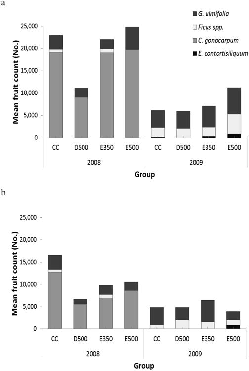
Mean July–August fruit counts for each group territory of Aotus azarae in the ranch Estancia Guaycolec of Argentina during the dry seasons of 2008 and 2009. (a) 80 % home range areas. (b) 50 % core areas. Modified from Fernandez-Duque and van der Heide, 2013.

A relatively infrequent drought during Nov-Dec 2008 and Jan-Apr 2009 (385mm) offered an unplanned opportunity to evaluate the prediction under harsher conditions. Mean fruit production in the 2009 dry season was a third of that in the 2008 dry season for both the 80% home range and the 50% core areas. One of the most abundant dry season fruiting sources (Chrysophyllum gonocarpum) did not fruit at all in 2009. This resulted in absolute differences in mean fruit production among 80% territories that were small, and among the 50% core areas even smaller (Fig. 2b). The changes in food availability in 2008 and 2009 were followed by corresponding changes in feeding patterns (Table I in Fernandez-Duque and van der Heide, 2013). Groups consumed almost no Chrysophyllum gonocarpum fruits (2008: 24.3% vs 2009: 1.9%), and increased their consumption of Guazuma ulmifolia (2008: 10.9% vs 2009: 17.9%), Ficus spp. fruits (2008: 16.0% vs 2009: 32.5%), and liana and vine leaves (2008: 0.65% vs 2009: 9.9%). Given that there were no pronounced differences, in absolute terms, between the fruit produced by the 80% home ranges and the core areas, the data suggest that it is the core areas of exclusive use that are more productive in this harsh dry season than the rest of their ranges.

Group demography and life-history traits

Prediction 7

The strongest evidence in support of the hypothesis would be data showing a causal relationship between resource distribution, ranging patterns and the reproductive success of the individuals in a socially monogamous relationship. In other words, one expects that groups inhabiting home ranges with higher resource availability would exhibit increased reproductive success. If resources determine the distribution of females and subsequently males, females should have higher reproductive success where resources are more abundant; variation in resource availability among ranges should predict variation in reproductive success among groups.

There are several demographic parameters and life-history traits that can be evaluated as proxies for reproductive success. First, assuming that the number of infants produced is directly related to the nutritional status of females, which is related to available food, different predictions can be made depending on whether one considers the entire home range or the core area, as the most relevant area to consider. Under the hypothesis being considered, the prediction is that the number of infants produced in different home ranges will vary minimally. If one found that breeders in one range are producing, for example, three times as many infants as another, this observation would be hard to reconcile with a proposition that the available food (and therefore energy for reproduction) is similar in all areas.

An analysis of infant production in four home ranges during nine years found that infants in those ranges were born in 71-75% of the years (i.e. relatively equal among groups) [Table 1, van der Heide et al., 2012]. When considering a 17-year period, those four ranges showed more variation in infant production, with some groups producing infants in 56% of study years and others producing in 76% of study years (Table 4); a similar pattern was found when the 10 groups (including the four indicated above) studied in the central area of study were examined during 14-17 birth seasons. Among these breeders, some produced offspring during 29% of study years whereas others produced offspring during 88% of study years (Table 4). Finally, the examination of infant production in 19 home ranges showed the largest differences in the number of infants born per group (29-90%, Table 4).

Infant production was not strongly related to 90% home range or 50% core areas. When the best studied groups were considered (central area groups, n=10, Table 4), the relationship with home range area was small (r=0.22) and with the core area even smaller (r=0.07, Table 6). The analyses of all groups (n=19) also showed small, and negative relationships for the home range (r=-0.11) and the core area (r=-0.19).

Table 6. Correlations between the size of the home range and core areas and life-history parameters for intensively studied groups (central groups) and all groups combined.

			Infant Production	Infant Mortality	Juvenile Disappearance	Age at Dispersal
Home Range	Central groups (n=10)	Pearson Correlation	0.22	-0.21	0.43	0.12
		Sig. (2-tailed)	0.5	0.6	0.2	0.7
	All groups (n=19)	Pearson Correlation	-0.11	-0.24	0.06	-0.07
		Sig. (2-tailed)	0.7	0.3	0.8	0.8
Core Area	Central groups (n=10)	Pearson Correlation	0.07	0.18	0.33	0.40
		Sig. (2-tailed)	0.8	0.6	0.3	0.3
	All groups (n=19)	Pearson Correlation	-0.19	-0.15	0.00	-0.03
		Sig. (2-tailed)	0.4	0.5	1.0	0.9

Prediction 8

The quality of a home range also can influence infant (0-6 months) and juvenile (6-16 months) mortality under the assumption that access to food resources is linked to the health and survival of both the mother and her young. Thus, I predict that there will be no marked differences in infant and juvenile mortality among home ranges.

In the previous analysis and here we assume that the disappearance of an infant (0-6 months) or a juvenile [6-16 months, Huck et al., 2011] can be attributed to the death of that individual within the group, since we have never recorded animals dispersing when they were younger than 22 months of age [Fernandez-Duque, 2009]. A previous analysis found that infant mortality varied between 11-14% per group during 12 birth seasons [n=4 groups, van der Heide et al., 2012]. The analysis of the 10 central groups showed larger variation in infant mortality (8-27% per group) and the variation was at a maximum when all 19 groups were considered (0-44%). The disappearance of juveniles varied between 8-50% among the central groups, 0-44% among the peripheral groups and between 0-50% when all groups were considered (Table 4). Despite individual variation among groups, no clear pattern emerged with regards to the relationship between infant mortality and home range or core area (Table 6). For both the central groups and all groups together, the relationships were all small, negative or positive (Table 6).

Prediction 9

If home ranges had similar amounts of resources, the prediction is that they should support similar numbers of individuals which should result in similar group sizes. In other words, I assume that group size can be used as a proxy for examining the quality of the range. Over the years we have conducted several analyses of the relationship between group size and home range area. An examination of average group size in six groups during 10 years showed that differences in size among groups were pronounced and statistically significant [Wartmann et al., 2014]. The largest group had 4.2 individuals (± 0.8, N=10 years, whereas the smallest one only had 2.9 (± 0.6, N=10). A second study also found that four groups varied in size between 3.1 and 4.0 individuals [van der Heide, 2012], but group size was not a strong predictor of the size of the annual range or core area.

Prediction 10

Owl monkeys disperse from their natal groups when they are on average 3 years old. We have shown that there is a tendency for dispersal to be more frequent during September-March, with a peak during October, and this is a period that coincides both with an abundance of food and the birth season [Fernandez-Duque, 2009]. The mechanisms regulating natal dispersal are still somewhat unclear [Huck and Fernandez-Duque, 2012], but one hypothesis is that the age at which individuals disperse from their natal groups may be partially influenced by competition for food resources within the group. Under this assumption, one would expect similar ages at dispersal if there were no differences among home ranges in the resources available to predispersing individuals.

Two separate analyses found relatively small differences in the median age at natal dispersal (Table 4). A first analysis of four central groups showed that the difference in the mean age at dispersal between groups was four months [van der Heide et al., 2012]. The analysis presented here of all 19 groups shows a larger range of variation in the mean age of natal dispersal (2.1 to 4.1 years, Table 4). The variation was markedly less for the central groups for which natal dispersal events were more precisely timed (2.1 to 3.5 years). For the periphery groups this variation was between 2.4 and 4.1 years. As with infant production and mortality, the size of the home range was not a good predictor of age of natal dispersal (Table 6). The relationship between the size of the core area and age of dispersal for the central groups showed the strongest of all relationships considered (r=0.40), possibly implying group size and intragroup competition as relevant factors influencing dispersal.

Discussion

I have evaluated the hypothesis that considers social monogamy in owl monkeys as a default social system imposed upon males because the spatial and/or temporal distribution of resources and females makes it difficult for single males to maintain access to more than one mate. I have tried to do this relying on a combination of data sets that explore ranging patterns and use of space, the spatial and temporal distribution of actual and potential food, and demographic and life-history variables that should be informative measures of the actual reproductive success of individuals.

The ranging patterns results do not provide support for the predictions that socially monogamous owl monkey groups make similar use of space (P1 and P3). In our population, groups occupy home ranges and core areas that vary substantially in size; males in some groups inhabit areas that would allow them to range over the areas occupied by two, and sometimes even three breeding females. The variation in the size of the core areas used by groups is relatively smaller, consistent with the idea that it may be the core areas that are the functionally relevant unit of analysis for exploring a possible connection between social monogamy and the temporal availability of resources. Understanding the extent and determinants of overlap in the home ranges and core areas among owl monkey groups will probably be valuable for explaining the evolution and maintenance of social monogamy. In our studies, we found that the overlap between home ranges was pronounced (48 ± 15%, Figure 4, Wartmann et al., 2014), whereas the core areas showed limited overlap (11 ± 15%). Owl monkey 50% core areas are approximately 30% the size of the annual range, which means that owl monkeys spend, on average, half of their time in a third of their range.

The results on ranging and use of space need to be considered with caution since our current estimates of home range and core area size and overlap are the consequence of movements while feeding, mating, sleeping, drinking, socializing and/or escaping predators. The data I have presented summarize the use of space for the exploitation of all resources combined, without considering other relevant factors. An important improvement in research design will be to conduct analyses for other resources in the home range such as sleeping sites or trees that provide adequate protection from predators, heat or cold; resources that may be distributed in a manner that influences the distribution of females in space. For example, the ranging behavior of white-headed langurs and red-fronted lemurs was strongly influenced by access to water holes during the dry season [Scholz and Kappeler, 2004; Zhou et al., 2011], and sleeping sites were found to have a non-random distribution in two species of tamarins with more sleeping sites found in the central area of the range than in the periphery [Smith et al., 2007]. We are currently beginning to examine sleeping tree abundance and distribution in the exclusive and overlap portions of each home range [Savagian et al., 2014] and we have found that sleeping trees are not distributed evenly throughout a group's home range, they are more likely to be located within 20m of a feeding tree.

Similarly important, we have not yet distinguished in our analyses ranging data points collected in the context of social interactions from those collected when the animal was foraging. For example, at dawn and dusk, during their peaks of activity, owl monkeys sometimes travel fast to the periphery of their home ranges, in what we normally interpret as a willingness to interact with other neighboring groups or floaters roaming the area. Future research should collect spatial data that identify the context in which this ranging occurs. If one found that certain areas of the home range are more frequently used for feeding than others (e.g. central area vs periphery), then it is likely that the core areas represent the “unit” on which to conduct analyses of the relationship between ranging, food availability and monogamy, with the periphery acting as some type of buffer zone.

The results from testing the three predictions related to the distribution of food (P4, P5, P6) offered valuable insights into understanding the functioning and maintenance of owl monkey monogamy. First, our data strongly suggest that there are important differences in the potential food availability among home ranges, those differences being larger among the 80% ranges than the core areas (P.4). Larger ranges had a greater potential to produce fruits, flowers and leaves than the smaller ranges. The analysis of actual food availability proved even more informative; there were indications that the availability of actual food sources in the core areas during the dry season may be of substantial importance in regulating social monogamy in owl monkeys if they provide the groups with the minimum nutritional requirements at times of limited food availability. These findings on food availability in the core area highlight the relevance of analyzing ranging patterns across specific microhabitats, or zones of use, to further understand how owl monkeys may be differentially using core areas and home ranges. In other words, if the core area represents a zone of exclusive use that provides the critical food resources, it may be the core area that needs to be examined when exploring the relationship between a socially monogamous mating system and ecology. Future analyses will need to more precisely define the spatial (e.g. annual range, core area, seasonal range), and the temporal (e.g. seasons, one year, multi-year) scale over which food resources are critical to structuring primate social and mating systems. In the case of owl monkeys, it will be necessary to explore the availability of actual food sources in the core areas during the dry season, when conceptions occur.

Finally, none of the proxies for the reproductive success of groups were strongly related to the size of the home range or core area. The predictions formulated to examine the relationship between demography and life history with the use of space and resources (P7, P8, P9, P10), did not indicate any strong differences among groups. Infant production, infant and juvenile mortality, age at dispersal and group size all varied among groups, but none showed a strong relationship to the size of the home range or core area. These findings are similar to those reported in a study of flexible pair-living white-handed gibbons (Hylobates lar), no differences existed among groups in most measures of gibbon reproductive performance [Savini et al., 2008]. Still, despite these results, it seems unlikely that the availability of resources in the range and the reproductive success of the individuals inhabiting that portion of the forest are not causally linked in some manner. It is, in my opinion, more likely that our studies are not fine-grained enough in identifying the variables to measure and/or we are failing to appreciate the fact that small differences in individual reproductive success may have relevant long-term genetic and evolutionary effects on a population.

There also is a need to consider other factors that may be interacting with food and space, such as the history of each group and its influence on demographic and life history parameters. In this population, adult owl monkeys are frequently expelled from their groups by solitary intruders [Fernandez-Duque and Huck, 2013] and when this occurs the new pair usually does not produce an infant in the following birth first season. The replacement of one member of a breeding pair in this population occurs with similar rates for males and females (27 female and 23 male replacements in 149 group/years, n=18 groups). The process of natal dispersal also may be affected by a replacement. For example, female offspring tend to disperse sooner when their mothers are replaced than when a step-father has entered the group [Huck and Fernandez-Duque, 2012]. There is research suggesting that male mate defense and female resource defense may be important mechanisms of maintaining social monogamy in hylobatids [Borries et al., 2011; Mitani, 1984; Mitani, 1987; Raemaekers and Raemaekers, 1985; Sommer, 2000]. There also are studies showing that ranging patterns alone cannot fully explain social monogamy in gibbons (Hylobates lar), fat-tailed dwarf lemurs (Cheirogaleus medius) and dik-diks (Madoqua kirkii) [Brotherton and Manser, 1997; Dunbar, 1988; Fietz, 2003; Reichard, 2003]. Second, it also is possible that some of the recorded differences may be evolutionarily important, even when statistically non-significant [Anderson, 2000; Burnham and Anderson, 2002; Garamszegi et al., 2009]. This is an extremely important consideration that continues to be largely ignored in the “small sample paradigm” characteristic of field primatology, despite an extensive literature on the topic [Cohen, 1994; Colqhuon, 2014; Fernandez-Duque, 1997; Ziliak and McCloskey, 2013]. Much of the time we lack adequate biological information on the consequences that a change in the variable of interest may cause and an exclusive reliance on the statistical significance of a test may prove uninformative at best if not misleading. For example, one of our studies found that the difference in mean age of dispersal between groups (5 months) occupying ranges of different size was not statistically significant [van der Heide et al. 2012]. Still, given that 83% of dispersal events in the population usually occur in a 6-month period [Fernandez-Duque, 2009], it seems reasonable to predict that a 5-month difference may have profound biological significance in the ability of a dispersing individual to usurp a breeding position in a neighboring group. One cannot disregard the possibility that similar limitations may exist in the analyses of other variables considered here.

In conclusion, when examining the validity of the various hypotheses advanced for explaining social monogamy (or any other aspect of primate behavior and ecology) we should be aware of the limitations of our research approach. Almost all of our research is observational, focused only on one or a few factors known to influence behavior and almost always structured to confirm hypotheses, not falsify them [Barlow, 1988; Taborsky, 2008]. Three recent analyses, which reach somewhat different conclusions, only offered correlational results with regards to the evolution of social monogamy in primates [Lukas and Clutton-Brock, 2014; Opie et al., 2013] and mammals [Lukas and Clutton-Brock, 2013]. Another examination of 64 mammalian species led the authors [Dobson et al., 2010] to conclude that it may be a futile exercise to attempt finding a general explanation for social monogamy among mammals, and instead it is likely that there will be different hypotheses explaining social monogamy in the different taxa. Our data are not detailed enough for explaining the evolution of social monogamy in owl monkeys, but they contribute to understanding how it is functioning. When examined in the general theoretical framework of hypotheses proposed to explain the evolution of social and mating systems in primates, these data will be valuable to help us formulate, in the future, quantitative and directional predictions that may bring us closer to identifying causal relationships regulating social monogamy in owl monkeys. I find these less than conclusive answers both a source of motivation for continuing our work and a source of reassurance that some debates on the evolution of social monogamy in primates, tacitly considered closed [Opie et al., 2013], may only be so on the surface [de Waal and Gavrilets, 2013; Dixson, 2013].

References

- Anderson DR. Null hypothesis testing: problems, prevalence and an alternative. Journal of Wildlife Management. 2000;64(4):912–923. [Google Scholar]
- Arditi SI. Variaciones estacionales en la actividad y dieta de Aotus azarae y Alouatta caraya en Formosa. 1. Vol. 3. Argentina: Boletín Primatológico Latinoamericano; 1992. pp. 11–30. [Google Scholar]
- Barlow GW. Monogamy in relation to resources. In: Slobodchikoff CN, editor. The Ecology of Social Behavior. London: Academic Press, Inc.; 1988. pp. 55–79. [Google Scholar]
- Borries C, Savini T, Koenig A. Social monogamy and the threat of infanticide in larger mammals. Behavioral Ecology and Sociobiology. 2011;65(4):685–693. [Google Scholar]
- Brotherton PNM, Komers PE. Mate guarding and the evolution of social monogamy in mammals. In: Reichard UH, Boesch C, editors. Monogamy Mating strategies and partnerships in birds, humans and other mammals. Cambridge: University of Cambridge; 2003. pp. 42–58. [Google Scholar]
- Brotherton PNM, Manser MB. Female dispersion and the evolution of monogamy in the dik-dik. Animal Behaviour. 1997;54(6):1413–1424. doi: 10.1006/anbe.1997.0551. [DOI] [PubMed] [Google Scholar]
- Brown AD, Placci LG, Grau NR. Ecología y diversidad de las selvas subtropicales de la Argentina. In: Goin F, Goni R, editors. Elementos de Política Ambiental. La Plata, Argentina: Di Giovanni Grafica; 1993. pp. 215–222. [Google Scholar]
- Burnham KP, Anderson DR. Model Selection and Multimodel Inference A Practical Information-Theoretic Approach. New York: Springer-Verlag; 2002. [Google Scholar]
- Chapman CA, Rothman JM, Lambert JE. In: Food as a selective force in primates. Call J, Kappeler P, Palombit R, Silk J, Mitani J, editors. Primate Societies: University of Chicago Press; 2012. pp. 149–168. [Google Scholar]
- Cohen J. The Earth Is Round (p<.05) Am Psychol. 1994;49(12):997–1003. [Google Scholar]
- Colqhuon D. An investigation of the false discovery rate and the misinterpretation of p-values. Royal Society Open Science. 2014;1:140216. doi: 10.1098/rsos.140216. [DOI] [PMC free article] [PubMed] [Google Scholar]
- de Waal F, Gavrilets S. Monogamy with a purpose. Proceedings of the National Academy of Sciences. 2013;110(38):15167–15168. doi: 10.1073/pnas.1315839110. [DOI] [PMC free article] [PubMed] [Google Scholar]
- Dixson AF. Male infanticide and primate monogamy. Proceedings of the National Academy of Sciences of the United States of America. 2013;110(51):E4937. doi: 10.1073/pnas.1318645110. [DOI] [PMC free article] [PubMed] [Google Scholar]
- Dobson SF, Way BM, Baudoinc C. Spatial dynamics and the evolution of social monogamy in mammals. Behavioral Ecology. 2010;21(4):747–752. [Google Scholar]
- Dunbar RIM. Primate Social Systems. Ithaca, New York: Cornell University Press; 1988. p. 373. [Google Scholar]
- Dunbar RIM. The mating system of the callitrichid primates: I. Conditions for the coevolution of pair bonding and twinning. Animal Behaviour. 1995;50:1057–1070. [Google Scholar]
- Emlen ST, Oring LW. Ecology, sexual selection, and the evolution of mating systems. Science. 1977;197(4300):215–223. doi: 10.1126/science.327542. [DOI] [PubMed] [Google Scholar]
- Fernandez-Duque E. Comparing and combining data across studies: alternatives to significance testing. Oikos. 1997;79(3):616–618. [Google Scholar]
- Fernandez-Duque E. Influences of moonlight, ambient temperature and food availability on the diurnal and nocturnal activity of owl monkeys (Aotus azarai) Behavioral Ecology and Sociobiology. 2003;54(5):431–440. [Google Scholar]
- Fernandez-Duque E. Natal dispersal in monogamous owl monkeys (Aotus azarai) of the Argentinean Chaco. Behaviour. 2009;146:583–606. [Google Scholar]
- Fernandez-Duque E. Rensch's rule, Bergman's effect and adult sexual dimorphism in wild monogamous owl monkeys (Aotus azarai) of Argentina. American Journal of Physical Anthropology. 2011;146:38–48. doi: 10.1002/ajpa.21541. [DOI] [PubMed] [Google Scholar]
- Fernandez-Duque E. The Aotinae: social monogamy in the only nocturnal anthropoid. In: Campbell CJ, Fuentes A, MacKinnon KC, Bearder SK, Stumpf RM, editors. Primates in Perspective. Second. Oxford: Oxford University Press; 2011. pp. 140–154. [Google Scholar]
- Fernandez-Duque E, de la Iglesia H, Erkert HG. Moonstruck primates: owl monkeys (Aotus) need moonlight for nocturnal activity in their natural environment. PLoS ONE. 2010;5(9):e12572. doi: 10.1371/journal.pone.0012572. [DOI] [PMC free article] [PubMed] [Google Scholar]
- Fernandez-Duque E, Huck M. Till death (or an intruder) do us part: intra-sexual competition in a monogamous primate. PLoS One. 2013;8(1):e53724. doi: 10.1371/journal.pone.0053724. [DOI] [PMC free article] [PubMed] [Google Scholar]
- Fernandez-Duque E, Rotundo M. Field methods for capturing and marking Azarai night monkeys. International Journal of Primatology. 2003;24(5):1113–1120. [Google Scholar]
- Fernandez-Duque E, Rotundo M, Ramírez-Llorens P. Environmental determinants of birth seasonality in night monkeys (Aotus azarai) of the Argentinean Chaco. International Journal of Primatology. 2002;23(3):639–656. [Google Scholar]
- Fernandez-Duque E, Rotundo M, Sloan C. Density and population structure of owl monkeys (Aotus azarai) in the Argentinean Chaco. American Journal of Primatology. 2001;53(3):99–108. doi: 10.1002/1098-2345(200103)53:3<99::AID-AJP1>3.0.CO;2-N. [DOI] [PubMed] [Google Scholar]
- Fernandez-Duque E, van der Heide G. Getting through the winter: dry season resources and their influence on owl monkey reproduction. International Journal of Primatology 2013 [Google Scholar]
- Fietz J. Pair living and mating strategies in the fat-tailed dwarf-lemur (Cheirogaleus medius) In: Reichard UH, Boesch C, editors. Monogamy Mating strategies and partnerships in birds, humans and other mammals. Cambridge: University of Cambridge; 2003. pp. 214–231. [Google Scholar]
- Fuentes A. Re-evaluating primate monogamy. American Anthopologist. 1999;100(4):890–907. [Google Scholar]
- Garamszegi LZ, Calhim S, Dochtermann NA, Hegyi G, Hurd PL, Jorgensen C, Kutsukake N, Lajeunesse MJ, Pollard KA, Schielzeth H, et al. Changing philosophies and tools for statistical inferences in behavioral ecology. Behavioral Ecology. 2009;20(6):1363–1375. [Google Scholar]
- Garber PA, Porter LM, Spross J, Di Fiore A. Saddleback tamarins: insights into monogamous and non-monogamous single female breeding systems. American Journal of Primatology. doi: 10.1002/ajp.22370. this volume. [DOI] [PubMed] [Google Scholar]
- García JE, Braza F. Densities comparisons using different analytic-methods in Aotus azarae. Primate Report. 1989;25:45–52. [Google Scholar]
- Giménez M, Fernandez-Duque E. Summer and Winter diet of night monkeys in the gallery and thorn forests of the Argentinean Chaco. Revista de Etología. 2003;5(164) [Google Scholar]
- Giménez MC. Dieta y comportamiento de forrajeo en verano e invierno del mono mirikiná (Aotus azarai azarai) en bosques secos y húmedos del Chaco Argentino [Licenciate] Buenos Aires: University of Buenos Aires; 2004. p. 57. [Google Scholar]
- Heltne PG. Census of Aotus in Northern Colombia. Washington, D.C.: Panamerican Health Organization; 1977. pp. 1–11. [Google Scholar]
- Huck M, Fernandez-Duque E, Babb PL, Schurr TG. Correlates of genetic monogamy in pair-living mammals: Insights from monogamous Azara's owl monkeys. Proceedings of the Royal Society B. 2014a;281 doi: 10.1098/rspb.2014.0195. [DOI] [PMC free article] [PubMed] [Google Scholar]
- Huck MG, Fernandez-Duque E. Children of divorce: effects of adult replacements on previous offspring in Argentinean owl monkeys. Behavioral Ecology and Sociobiology. 2012;66(3):505–517. [Google Scholar]
- Huck MG, Rotundo M, Fernandez-Duque E. Growth, development and age categories in male and female wild monogamous owl monkeys (Aotus azarai) of Argentina. International Journal of Primatology. 2011;32:1133–1152. [Google Scholar]
- Huck MG, van Lunenburg M, Dávalos V, Rotundo M, Di Fiore A, Fernandez-Duque E. Double effort: parental behaviour of wild Azara's owl monkeys in the face of twins. American Journal of Primatology. 2014b doi: 10.1002/ajp.22256. [DOI] [PubMed] [Google Scholar]
- Irwin MT, Raharison JL, Raubenheimer D, Chapman CA, Rothman JM. Nutritional correlates of the “lean season”: effects of seasonality and frugivory on the nutritional ecology of diademed sifakas. Am J Phys Anthropol. 2014;153(1):78–91. doi: 10.1002/ajpa.22412. [DOI] [PubMed] [Google Scholar]
- Janson C. Reconciling rigor and range: observations, experiments, and quasi-experiments in field primatology. International Journal of Primatology. 2012;33:520–541. [Google Scholar]
- Juárez C, Fernandez-Duque E. IV Reunión Binacional de Ecología. Buenos Aires, Argentina: 2010. Efecto de la fragmentación natural del habitat en la estructura de la poblacion del mono mirikiná (Aotus azarai) en el chaco humedo formoseño. [Google Scholar]
- Juárez CP. Demografía e historia de vida del mono mirikiná (Aotus a azarai) en el Chaco Húmedo Formoseño [Doctoral Dissertation] Tucumán: Universidad Nacional de Tucumán; 2012. [Google Scholar]
- Juárez CP, Baldovino C, Kowaleski M, Fernandez-Duque E. Los Primates de Argentina: Ecología y Conservación. Manejo de Fauna en la Argentina: Acciones para la Conservación de Especies Amenazadas: Fundación de Historia Natural ‘Felix de Azara’ 2012 [Google Scholar]
- Kappeler PM. Lemur behaviour informs the evolution of social monogamy. Trends Ecol Evol. 2014;29(11):591–3. doi: 10.1016/j.tree.2014.09.005. [DOI] [PubMed] [Google Scholar]
- Kleiman DG. Monogamy in mammals. The Quarterly Review of Biology. 1977;52:39–69. doi: 10.1086/409721. [DOI] [PubMed] [Google Scholar]
- Komers PE. Obligate monogamy without paternal care in Kirk's dikdik. Animal Behaviour. 1996;51(1):131–140. [Google Scholar]
- Komers PE, Brotherton PNM. Female space use is the best predictor of monogamy in mammals. Proceedings of the Royal Society of London Series B: Biological Sciences. 1997;264:1261–1270. doi: 10.1098/rspb.1997.0174. [DOI] [PMC free article] [PubMed] [Google Scholar]
- Lukas D, Clutton-Brock T. Evolution of social monogamy in primates is not consistently associated with male infanticide. Proc Natl Acad Sci U S A. 2014;111(17):E1674. doi: 10.1073/pnas.1401012111. [DOI] [PMC free article] [PubMed] [Google Scholar]
- Lukas D, Clutton-Brock TH. The evolution of social monogamy in mammals. Science. 2013;341(6145):526–30. doi: 10.1126/science.1238677. [DOI] [PubMed] [Google Scholar]
- Lukas D, Huchard E. The evolution of infanticide by males in mammalian societies. Science. 2014;346:841–844. doi: 10.1126/science.1257226. [DOI] [PubMed] [Google Scholar]
- Mason WS, Mendoza SP. Generic sspects of primate attachments: parents, offspring and mates. Psychoneuroendocrinology. 1998;23:765–778. doi: 10.1016/s0306-4530(98)00054-7. [DOI] [PubMed] [Google Scholar]
- Mitani JC. The behavioral regulation of monogamy in gibbons (Hylobates muelleri) Behavioral Ecology and Sociobiology. 1984;15:225–229. [Google Scholar]
- Mitani JC. Territoriality and monogamy among agile gibbons (Hylobates agilis) Behavioral Ecology and Sociobiology. 1987;20:265–269. [Google Scholar]
- Möller AP. The evolution of monogamy: mating relationships, parental care and sexual selection. In: Reichard UH, Boesch C, editors. Monogamy Mating strategies and partnerships in birds, humans and other mammals. Cambridge: University of Cambridge; 2003. pp. 29–41. [Google Scholar]
- Neiff JJ. Bosques fluviales de la cuenca del Paraná. In: Arturi MF, Frangi JL, Goya JF, editors. Ecología y manejo de los bosques de Argentina La Plata. Servicio de Difusion de la Creacion Intelectual de la Universidad Nacional de La Plata: Editorial de la Universidad Nacional de La Plata (EDULP); 2005. [Google Scholar]
- Opie C, Atkinson QD, Dunbar RI, Shultz S. Male infanticide leads to social monogamy in primates. Proceedings of the National Academy of Sciences of the United States of America. 2013;110(33):13328–32. doi: 10.1073/pnas.1307903110. [DOI] [PMC free article] [PubMed] [Google Scholar]
- Placci G. Estructura y funcionamiento fenológico en relación a un gradiente hídrico en bosques del este de Formosa [Tesis Doctoral] La Plata: Universidad Nacional de la Plata; 1995. [Google Scholar]
- Raemaekers JJ, Raemaekers PM. Field playback of loud calls to gibbons (Hylobates lar): territorial, sex-specific and species-specific responses. Animal Behaviour. 1985;33:481–493. [Google Scholar]
- Reichard U. Social monogamy in gibbons: the male perspective. In: Reichard UH, Boesch C, editors. Monogamy Mating strategies and partnerships in birds, humans and other mammals. Cambridge: University of Cambridge; 2003. pp. 190–213. [Google Scholar]
- Rutberg AT. The evolution of monogamy in primates. Journal of Theoretical Biology. 1983;104:93–112. doi: 10.1016/0022-5193(83)90403-4. [DOI] [PubMed] [Google Scholar]
- Savagian A, Twitchell-Heyne A, Corley M, Rotundo M, Di Fiore A, Fernandez-Duque E. Resource utilization and home range overlap in territorial owl monkeys of Argentina. American Journal of Physical Anthropology. 2014;153(S58):230. [Google Scholar]
- Savini T, Boesch C, Reichard UH. Home-range characteristics and the influence of seasonality on female reproduction in white-handed gibbons (Hylobates lar) at Khao Yai National Park, Thailand. Am J Phys Anthropol. 2008;135(1):1–12. doi: 10.1002/ajpa.20578. [DOI] [PubMed] [Google Scholar]
- Scholz F, Kappeler P. Effects of seasonal water scarcity on the ranging behavior of Eulemur fulvus rufus. International Journal of Primatology. 2004;25(3):599–613. [Google Scholar]
- Smith AC, Knogge C, Huck M, Löttker P, Buchanan-Smith HM, Heymann EW, Smith AB. Long-term patterns of sleeping site use in wild saddleback (Saguinus fuscicollis) and mustached tamarins (S. mystax): effects of foraging, thermoregulation, predation, and resource defense constraints. American Journal of Physical Anthropology. 2007;134:340–353. doi: 10.1002/ajpa.20676. [DOI] [PubMed] [Google Scholar]
- Sommer S. Sex-specific predation on a monogamous rat, Hypogeomys antimena (Muridae: Nesomyinae) Animal Behaviour. 2000;59(6):1087–1094. doi: 10.1006/anbe.2000.1381. [DOI] [PubMed] [Google Scholar]
- Taborsky M. The use of theory in behavioural research. Ethology. 2008;114:1–6. [Google Scholar]
- Tecot S. this volume
- van der Heide GWE, Fernandez-Duque E, Iriart D, Juárez CP. Do forest composition and fruit availability predict demographic differences among groups of territorial owl monkeys (Aotus azarai)? International Journal of Primatology. 2012;33(1):184–207. [Google Scholar]
- van Schaik CP, van Hoof JARAM. On the ultimate causes of primate social systems. Behaviour. 1983;85:91–117. [Google Scholar]
- Wartmann FM, Juárez CP, Fernandez-Duque E. Size, site fidelity and overlap of home ranges and core areas in the socially monogamous owl monkey (Aotus azarae) of Northern Argentina. International Journal of Primatology 2014 [Google Scholar]
- Wittenberger JF, Tilson RL. The evolution of monogamy: hypotheses and evidence. Annual Review of Ecology and Systematics. 1980;11:197–232. [Google Scholar]
- Woodroffe R, Vincent A. Mother's little helpers: patterns of male care in mammals. Trends in Ecology and Evolution. 1994;9:294–297. doi: 10.1016/0169-5347(94)90033-7. [DOI] [PubMed] [Google Scholar]
- Zhou Q, Tang X, Huang H, Huang C. Factors Affecting the Ranging Behavior of White-headed Langurs (Trachypithecus leucocephalus) International Journal of Primatology. 2011;32:511–523. [Google Scholar]
- Ziliak ST, McCloskey DN. We Agree That Statistical Significance Proves Essentially Nothing: A Rejoinder to Thomas Mayer. Econ Journal Watch. 2013;10(1):97–+. [Google Scholar]