Dynamic behaviors of a modified SIR model in epidemic diseases using nonlinear incidence and recovery rates

Abstract

The transmission of infectious diseases has been studied by mathematical methods since 1760s, among which SIR model shows its advantage in its epidemiological description of spread mechanisms. Here we established a modified SIR model with nonlinear incidence and recovery rates, to understand the influence by any government intervention and hospitalization condition variation in the spread of diseases. By analyzing the existence and stability of the equilibria, we found that the basic reproduction number ${\mathbb{R}}_0$ is not a threshold parameter, and our model undergoes backward bifurcation when there is limited number of hospital beds. When the saturated coefficient a is set to zero, it is discovered that the model undergoes the Saddle-Node bifurcation, Hopf bifurcation, and Bogdanov-Takens bifurcation of codimension 2. The bifurcation diagram can further be drawn near the cusp type of the Bogdanov-Takens bifurcation of codimension 3 by numerical simulation. We also found a critical value of the hospital beds b_c at ${\mathbb{R}}_0<1$ and sufficiently small a, which suggests that the disease can be eliminated at the hospitals where the number of beds is larger than b_c. The same dynamic behaviors exist even when a ≠ 0. Therefore, it can be concluded that a sufficient number of the beds is critical to control the epidemic.

Introduction

Since the development of the first dynamic model of smallpox by Bernoulli in 1760, various mathematical models have been employed to study infectious diseases [1] in order to reveal the underlying spread mechanisms that influence the transmission and control of these diseases. Among them, Kermack and Mckendrick [2] initiated a famous SIR type of compartmental model in 1927 for the plague studies in Mumbai, and succeed in unveiling its epidemiological transition. Since then, mathematical modeling has become an important tool to study the transmission and spread of epidemic diseases.

In the modeling of infectious diseases, the incidence function is one of the important factors to decide the dynamics of epidemic models. Bilinear and standard incidence rates, both monotonically increasing functions of the total of infected class, have been frequently used in early epidemic models [3]. In those models, the dynamics of models are relatively simple and almost determined by the basic reproduction number ${\mathbb{R}}_0$: the disease will be eliminated if ${\mathbb{R}}_0<1$, otherwise, the disease will persist. However, intervention strategies, such as isolation, quarantine, mask-wearing and medical report about emerging infectious diseases, play an vital role in controlling the spread, sometimes contributing to the eradication of diseases. For instance, the SARS in 2003 and novel influenza pandemic in 2009 have been well controlled by taking these intervention actions [4–15]. Hence, it is essential to expand the modeling studies to the investigation of the combined effects of these major intervention strategies. The generalized models will provide further understanding of the transmission mechanisms, and modify guidelines for public health in control of the spread of infectious diseases.

In recent years, a number of compartmental models have been formulated to explore the impact of intervention strategies on the transmission dynamics of infectious diseases. If denote the total number of hospital individuals, exposed and infectious as N, E and I respectively, Liu et al [16], Cui et al [17, 18] used βe^−mI, $\beta e^{-{\alpha }_{1}E-{\alpha }_{2}I-{\alpha }_{3}H}$ and c₁ − c₂ f(I) to study the impact of media coverage on the dynamics of epidemic models, respectively. However, people may adjust their behaviors according to these government intervention. Therefore, Ruan and Xiao [19] set incidence function in the form of $f_1\left(I\right)S=\frac{KIS}{1+\alpha I^2}$(a special case of $\frac{k{I}^{p}S}{1+a{I}^q}$ [20, 21]) to include the above “psychological” effect: when the number of infectious individuals increases and is reported through social media, the susceptible individuals will stay alert spontaneously to reduce any unnecessary contact with others, thus lowering the contact and transmission incidence.

On the other hand, medical treatments, determining how well the diseases are controlled, are normally expressed as constant recovery rates in the current models. These recovery rates depend on various health systems and hospitalization conditions, such as the capacity of the hospitals and effectiveness of the treatments. Advanced models (see [22–24]) started to corporate the limited medical resources into the spread dynamics of infectious diseases. In the literature [22], Wang and Ruan first introduced a piece-wise treatment function in an SIR model,

$$\begin{array}{c}\hfill T\left(I\right)=\left\{\begin{array}{cc}r\hfill & I>0,\hfill \\ 0\hfill & I=0.\hfill \end{array}\right.\end{array}$$

where the maximal treatment capacity was used to cure infectives so that the epidemic of disease can be controlled. This situation occurs only if the infectious disease needs to be eliminated due to its threats to public. They discovered that the model undergoes Saddle-Node bifurcation, Hopf bifurcation and Bogdanov-Takens bifurcation, standing for the collision of two equilibria, the existance of periodic diseases, and two varying parameters in system, respectively. Wang [23] further modified the treatment rate to be proportinal to the number of infectives before the capacity of hospital was reached, by

$$\begin{array}{c}\hfill T\left(I\right)=\left\{\begin{array}{cc}rI\hfill & 0\le I\le I_0,\hfill \\ r{I}_0\hfill & I>I_0.\hfill \end{array}\right.\end{array}$$ (1)

The model was then found to perform backward bifurcation [23], indicating that the basic reproduction number was no longer a threshold.

In common hospital settings, the number of beds is an indicator of health resources, particularly the medical treatments of the infectives. Under this consideration, Shan and Zhu [24] defined the recovery rate as a function of b, the number of hospital beds, and I, the number of infectives.

$$\begin{array}{c}\hfill \mu =\mu (b,I)={\mu }_0+({\mu }_1-{\mu }_0){\displaystyle \frac{b}{I+b}}\end{array}$$ (2)

where μ₀ is the minimum per capita recovery rate, and μ₁ the maximum per capita recovery rate. They chose the standard incidence rate and discovered the complicated dynamics including Saddle-Node bifurcation, Backward bifurcation and Bogdanov-Takens bifurcation of codimension 3, which means that the recovery rate contributes to the rich dynamics of epidemic models.

Our strategy thus becomes, both government intervention and hospitalization condition need to be incorporated to achieve a better control of the emerging infectious. Therefore, the incidence rate is expressed as

$$\begin{array}{c}\hfill \beta \left(I\right)=\frac{\beta I}{a{I}^2+cI+1},\end{array}$$

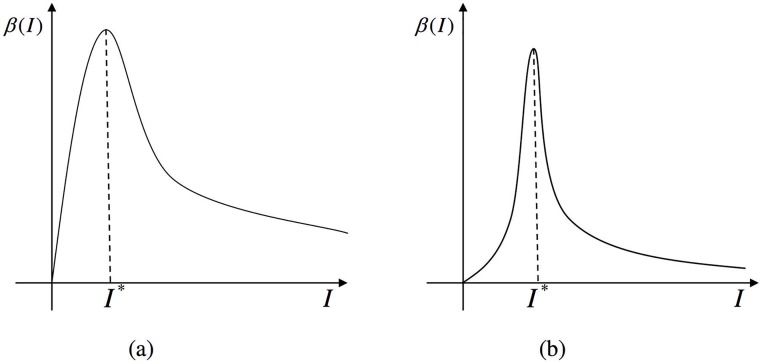
where a is positive constant and $c>-2\sqrt{a}$ (so that aI² + cI + 1 > 0 for all I > 0 and hence β(I) > 0 for all I > 0). When the threshold of the number of infected individuals I* is reached, the contact transmission rate starts to decrease as the number of infected individuals grows. As shown in Fig 1, the incidence β(I) increases to its maximum and then decreases to zero as I tends to infinity, which explains the phenomenon where the rate of contacting between infected I and susceptible S decreases after government intervention. We use the same expression of hospitalization conditions as the literature [24], and the following model is then established,

$$\begin{array}{c}\hfill \left\{\begin{array}{ccc}\hfill {\displaystyle \frac{dS}{dt}}& =& A-dS-{\displaystyle \frac{\beta SI}{1+cI+a{I}^2}},\hfill \\ \hfill {\displaystyle \frac{dI}{dt}}& =& {\displaystyle \frac{\beta SI}{1+cI+a{I}^2}}-dI-\alpha I-\mu (b,I)I,\hfill \\ \hfill {\displaystyle \frac{dR}{dt}}& =& \mu (b,I)I-dR,\hfill \end{array}\right.\end{array}$$ (3)

where A is the recruitment rate of the susceptible population, d the natural death of the population, and α the per capita disease-induced death rate, respectively.

Fig 1. Graphs of incidence rate function.

(a) c ≥ 0; (b) $-2\sqrt{a}<c<0$.

For system (3), the cone R³⁺ is a positive invariant. The C¹ smoothness of the right side of system (3) implies the local existence and uniqueness of the solution with initial values in R³⁺. Adding up the three equations of system (3), we get N′(t) = A − dN − αI. Therefore, all solutions in the first octant approach, entering or staying inside the set, are defined by

$$\begin{array}{c}\hfill D=\left\{(S,I,R)\right|S\ge 0,I\ge 0,R\ge 0,S+I+R\le \frac{A}{d}\}.\end{array}$$

This paper will be organized as follows. In section 2, we study the existence of the equilibria of our model. In section 3, we study the stability of the equilibria. In section 4, we examine the dynamics of the model by first looking at the backward bifurcation of system, then the much complicated Hopf bifurcation and Bogdanov-Takens bifurcation of codimension 2 and 3. We summarize our results and discuss the epidemiological significance of the number of hospital beds and intervention strategies in section 5.

Existence of equilibria

For simplicity we will focus on the case when c = 0. If c ≠ 0, but c is in small neighborhood of zero, the behaviors of model still exist. Our model thus becomes,

$$\begin{array}{c}\hfill \left\{\begin{array}{ccc}\hfill {\displaystyle \frac{dS}{dt}}& =& A-dS-{\displaystyle \frac{\beta SI}{1+a{I}^2}},\hfill \\ \hfill {\displaystyle \frac{dI}{dt}}& =& {\displaystyle \frac{\beta SI}{1+a{I}^2}}-dI-\alpha I-({\mu }_0+({\mu }_1-{\mu }_0){\displaystyle \frac{b}{b+I}})I,\hfill \\ \hfill {\displaystyle \frac{dR}{dt}}& =& ({\mu }_0+({\mu }_1-{\mu }_0){\displaystyle \frac{b}{b+I}})I-dR.\hfill \end{array}\right.\end{array}$$ (4)

Since the first two equations are independent of the third, it suffices to consider the first two equations. Thus, we will focus on the reduced model in the following discussions.

$$\begin{array}{c}\hfill \left\{\begin{array}{ccc}\hfill {\displaystyle \frac{dS}{dt}}& =& A-dS-\beta {\displaystyle \frac{SI}{1+a{I}^2}}\hfill \\ \hfill {\displaystyle \frac{dI}{dt}}& =& \beta {\displaystyle \frac{SI}{1+a{I}^2}}-dI-\alpha I-({\mu }_0+({\mu }_1-{\mu }_0){\displaystyle \frac{b}{b+I}})I.\hfill \end{array}\right.\end{array}$$ (5)

We find equilibria by setting the right hand of system (5) equal to zero:

$$\begin{array}{c}\hfill \left\{\begin{array}{cc}& A-dS-\beta {\displaystyle \frac{SI}{1+a{I}^2}}=0,\hfill \\ & \beta {\displaystyle \frac{SI}{1+a{I}^2}}-dI-\alpha I-\mu (b,I)I=0.\hfill \end{array}\right.\end{array}$$ (6)

Obviously, a trivial solution of Eq (6) is $E_0(S,I)=(\frac{A}{d},0)$, a disease free equilibrium(DFE). For E₀, by using the formula in [25], one can calculate the reproduction number

$$\begin{array}{c}\hfill {\mathbb{R}}_0=\frac{\beta A}{d(\alpha +d+{\mu }_1)}.\end{array}$$ (7)

For any positive equilibrium E(S, I), also called endemic equilibrium, when exists, its S and I coordinates satisfy

$$\begin{array}{c}\hfill S\left(I\right)=\frac{A-(d+\alpha +\mu (b,I\left)\right)I}{d},\end{array}$$ (8)

where the I coordinate will be the positive root of the following cubic equation

$$\begin{array}{c}\hfill f\left(I\right)=\mathcal{A}{I}^3+\mathcal{B}{I}^2+\mathcal{C}I+\mathcal{D}=0,\end{array}$$ (9)

where

$$\begin{array}{ll}\mathcal{A}=ad{\delta }_0,\hfill & \mathcal{B}=bad{\delta }_1+\beta {\delta }_0,\hfill \\ \mathcal{C}=\beta b{\delta }_1+d{\delta }_0-\beta A,\hfill & \mathcal{D}=bd{\delta }_1\left(1-{ℝ}_0\right),\hfill \\ {\delta }_i=d+\alpha +{\mu }_i,\hspace{1em}i=0,1.\hfill & \hfill \end{array}$$

Let

$$\begin{array}{c}\hfill A_1={\mathcal{B}}^2-3\mathcal{A}\mathcal{C},B=\mathcal{B}\mathcal{C}-9\mathcal{A}\mathcal{D},C={\mathcal{C}}^2-3\mathcal{B}\mathcal{D}\end{array}$$

Denote Δ₀ the discriminant of f(I) with respect to I, then

$$\begin{array}{c}\hfill {\Delta }_0=B^2-4A_{1}C.\end{array}$$

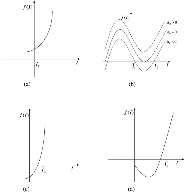
Note that $f\left(0\right)=bd{\delta }_1(1-{\mathbb{R}}_0)$ and $f\prime \left(0\right)=\mathcal{C}$. As shown in Fig 2, we have the following cases about the positive roots of f(I):

Fig 2. The positive roots of f(I).

(a) ${\mathbb{R}}_0<1,\mathcal{C}>0$; (b) ${\mathbb{R}}_0<1,\mathcal{C}<0$; (c) ${\mathbb{R}}_0>1,\mathcal{C}>0$; (d) ${\mathbb{R}}_0>1,\mathcal{C}<0$.

• Case 1:

  ${\mathbb{R}}_0>1$. In this case, $\mathcal{D}<0$. It is found that there is a unique positive root of f(I) = 0, regardless of the sign of C from Fig 1(c) and 1(d).

• Case 2:

  ${\mathbb{R}}_0<1$. In this case, $\mathcal{D}>0$. If $\mathcal{C}>0$, equation f(I) = 0 has no positive solution (see Fig 1(a)). If $\mathcal{C}<0$, similar to Lemma 2.1 described by Huang and Ruan [26], the following conclusions can be drawn as shown by Fig 1(b).

  • (a)Δ₀ < 0, there are two positive solutions of the equation.
  • (b)Δ₀ = 0, there is unique positive solution of the equation.
  • (c)Δ₀ > 0, we find that Eq (9) has no positive solution.
• Case 3:
  ${\mathbb{R}}_0=1$, Eq (9) becomes

  $$\begin{array}{c}\hfill f\left(I\right)=\mathcal{A}{I}^3+\mathcal{B}{I}^2+\mathcal{C}I=0\end{array}$$ (10)

  If $\mathcal{C}<0$, Eq (9) has a unique positive root. If $\mathcal{C}>0$, Eq (9) has no positive root. Note that $\mathcal{C}>0$ means $b>\frac{d({\mu }_1-{\mu }_0)}{\beta {\delta }_1}$. Thus, we get the following theorem about the equilibrium of the model.

Theorem 0.1. For system (5) with positive parameters,

• (1)the disease-free equilibrium E₀ always exists,
• (2)when ${\mathbb{R}}_0>1$, system has a unique endemic equilibrium,
• (3)when ${\mathbb{R}}_0<1$, and
  • (a)$\mathcal{C}>0$, system (5) does not have endemic equilibrium.
  • (b)$\mathcal{C}<0$, Δ₀ < 0, there exist two endemic equilibria $E_1({\overline{I}}_1,{\overline{S}}_1)$ and $E_2({\overline{I}}_2,{\overline{S}}_2)$, and when Δ₀ = 0 these two endemic equilibria coalesce into the same endemic equilibrium E*; otherwise system (5) has no endemic equilibrium.
• (4)when ${\mathbb{R}}_0=1$, there exists a unique endemic equilibrium if and only if $\mathcal{C}<0$ i.e. $b<\frac{d({\mu }_1-{\mu }_0)}{\beta {\delta }_1}$; otherwise there is no endemic equilibrium.

Remark 0.2. By calculation, we get that

$$\begin{array}{c}\hfill \begin{array}{ccc}{\Delta }_0\left(a\right)\hfill & =\hfill & -3{\beta }^2{\delta }_0\Delta +O\left(a\right),\hfill \\ \Delta \hfill & =\hfill & {\beta }^2{\delta }_1^2{b}^2+2\beta (2\beta A{\delta }_0-d{\delta }_0{\delta }_1-\beta A{\delta }_1)b+{(d{\delta }_0-\beta A)}^2.\hfill \end{array}\end{array}$$ (11)

When a is sufficiently small and tends to zero, the sign of Δ₀ will be determined by the zero power of a. Therefore, Δ₀(a) → Δ₀(0) = −3β²δ₀Δ as a → 0. In addition, Δ = 0 if and only if ${\mathbb{R}}_0={\mathbb{R}}_0^c$. Here

$$\begin{array}{c}\hfill {\mathbb{R}}_0^c=1-\frac{{\mathcal{C}}^2}{4\mathcal{B}bd(d+\alpha +{\mu }_1)}.\end{array}$$

Stability analysis of equilibria

In order to discuss the stability of equilibrium, we need the Jacobian matrix of system (5) at any equilibrium E(S, I). If we denote the Jacobian as J(E) = (j_ij)_2×2, i, j = 1, 2, then a straightforward calculation gives

$$\begin{array}{c}\hfill \begin{array}{ccc}& j_{11}=-d-\frac{\beta I}{1+a{I}^2},\hfill & j_{12}=-\frac{\beta S}{1+a{I}^2}+\frac{2a\beta S{I}^2}{{(1+a{I}^2)}^2},\hfill \\ & j_{21}=\frac{\beta I}{1+a{I}^2},\hfill & j_{22}=-{\delta }_0+\frac{\beta S}{1+a{I}^2}-\frac{2a\beta S{I}^2}{{(1+a{I}^2)}^2}+\frac{({\mu }_1-{\mu }_0)bI}{{(b+I)}^2}-\frac{({\mu }_1-{\mu }_0)b}{b+I}.\hfill \end{array}\end{array}$$ (12)

Firstly, we present a theorem about the disease-free equilibrium E₀(A/d, 0).

Theorem 0.3. E₀ is an attracting node if ${\mathbb{R}}_0<1$, and hyperbolic saddle if ${\mathbb{R}}_0>1$. When ${\mathbb{R}}_0=1$, E₀ is a saddle-node of codimension 1 if $b\ne \frac{d^2({\mu }_1-{\mu }_0)}{{\beta }^{2}A}$ and attracting semi-hyperbolic node of codimension 2 if $b=\frac{d^2({\mu }_1-{\mu }_0)}{{\beta }^{2}A}$.

Proof. For system (5), −d and ${\delta }_1({\mathbb{R}}_0-1)$ are two eigenvalues of J(E₀). So, E₀ is an attracting node if ${\mathbb{R}}_0<1$, and unstable if ${\mathbb{R}}_0>1$. When ${\mathbb{R}}_0=1$, the second eigenvalue becomes zero. In order to analyze the behavior of E₀, we linearize system (5) and use the transformation of $X=S+\frac{\beta A}{d^2}I$, Y = I,

$$\{\begin{array}{l}\frac{dX}{dt}=-dX+P\left(X,Y\right),\hfill \\ \frac{dY}{dt}=-\left(\frac{{\mu }_0-{\mu }_1}{b}+\frac{{\beta }^{2}A}{d^2}\right)Y^2+Q\left(X,Y\right),\hfill \end{array}$$ (13)

where P(X, Y) and Q(X, Y) represent the higher order terms. Obviously, E₀ is a saddle-node if $b\ne \frac{d^2({\mu }_1-{\mu }_0)}{{\beta }^{2}A}$. Otherwise, i.e., $b=\frac{d^2({\mu }_1-{\mu }_0)}{{\beta }^{2}A}$, applying the center manifold theorem, system (5) becomes

$$\{\begin{array}{l}\frac{dX}{dt}=-dX+P\left(X,Y\right),\hfill \\ \frac{dY}{dt}=-\left(\frac{\beta Aa}{d}+\frac{{\beta }^{3}A{\delta }_0}{d^3}\right)Y^3+Q_1\left(X,Y\right),\hfill \end{array}$$ (14)

where Q₁(X, Y) represents the higher order term. Thus, E₀ is an attracting semi-hyperbolic node of codimension 2.

Theorem 0.4. If dδ₀ > βA, E₀ is globally asymptotically stable.

Proof. If dδ₀ > βA, it is obvious that ${\mathbb{R}}_0<1$ and $\mathcal{C}>0$. From Theorem 0.1 and 0.3, E₀ is the unique attracting node of system (5). In order to prove that the disease free equilibrium E₀ is globally and asymptotically stable, we construct the following Liapunov function:

$$\begin{array}{c}\hfill V(S,I)=\frac{A}{d}(\frac{dS}{A}-ln\frac{dS}{A})+I.\end{array}$$ (15)

It is easy to discover that $E_0(\frac{A}{d},0)$ attains the global minimum of the function V(S, I), so V(S, I) > 0. Along system (5), it turns out:

$$\begin{array}{c}\hfill \dot{V}{|}_{(5)}=2A-dS-\frac{A^2}{dS}+\frac{\beta AI}{d(1+a{I}^2)}-(d+\alpha +\mu (b,I))I.\end{array}$$ (16)

Since μ(b, I) > μ₀ for all I ≥ 0, we have

$$\begin{array}{c}\hfill \dot{V}{|}_{(5)}\le 2A-dS-\frac{A^2}{dS}+\frac{(\beta A-d{\delta }_0)I-da{\delta }_0{I}^3}{d(1+a{I}^2)}\le 0.\end{array}$$ (17)

The equality $\dot{V}(S,I)=0$ if and only if at $E_0(\frac{A}{d},0)$. By Poincare-Bendixson theorem, theorem 0.4 is obvious.

Let $E(\overline{S},\overline{I})$ be any endemic equilibrium, one can verify that its characteristic equation can be written as

$$\begin{array}{c}\hfill {\lambda }^2-\text{tr}\left(J_E\right)\lambda +det\left(J_E\right)=0,\end{array}$$ (18)

where

$$\begin{array}{c}\hfill \begin{array}{c}\text{tr}\left(J_E\right)=-d+{\displaystyle \frac{{\mu }_1-{\mu }_0}{{(b+\overline{I})}^2}}b\overline{I}-(d+\alpha +\mu (b,\overline{I})){\displaystyle \frac{2a{\overline{I}}^2}{1+a{\overline{I}}^2}}-{\displaystyle \frac{\beta \overline{I}}{1+a{\overline{I}}^2}},\hfill \\ det\left(J_E\right)={\displaystyle \frac{\overline{I}}{{(b+\overline{I})}^2(1+a{\overline{I}}^2)}}(b+\overline{I})f^{\prime }\left(\overline{I}\right).\hfill \end{array}\end{array}$$ (19)

Obviously, the signs of the eigenvalues are determined by $f^{\prime }\left(\overline{I}\right)$ and tr(J_E). From Fig 2, we know that $f^{\prime }\left({\overline{I}}_1\right)<0,f^{\prime }\left({\overline{I}}_2\right)>0$, so E₁ is a hyperbolic saddle and E₂ is an anti-saddle. E₂ is an attracting node or focus, if tr(J_E) < 0; E₂ is a weak focus or a center, if tr(J_E) = 0; E₂ is a repelling node or focus, if tr(J_E) > 0. So we obtain the following theorem.

Theorem 0.5. For system (5), there are two endemic equilibria E₁, E₂ when ${\mathbb{R}}_0<1$ and Δ₀ < 0. Then the low endemic equilibrium E₁ is a hyperbolic saddle, and the higher endemic equilibrium E₂ is an anti-saddle. When ${\mathbb{R}}_0>1$ there is a unique endemic equilibrium, which is an anti-saddle.

Bifurcation analysis

Backward bifurcation

Theorem 0.6. When ${\mathbb{R}}_0=1$, system (5) undergoes backward bifurcation if $b<\frac{d({\mu }_1-{\mu }_0)}{\beta {\delta }_1}$; and system (5) undergoes forward bifurcation if $b>\frac{d({\mu }_1-{\mu }_0)}{\beta {\delta }_1}$.

Proof. For convenience of the proof, we suppose that the total number of the population is N(t). System (4) becomes the following system

$$\begin{array}{c}\hfill \left\{\begin{array}{c}{\displaystyle \frac{dI}{dt}}={\displaystyle \frac{\beta (N-I-R)I}{1+a{I}^2}}-dI-\alpha I-({\mu }_0+({\mu }_1-{\mu }_0){\displaystyle \frac{b}{b+I}})I,\hfill \\ {\displaystyle \frac{dR}{dt}}=({\mu }_0+({\mu }_1-{\mu }_0){\displaystyle \frac{b}{b+I}})I-dR,\hfill \\ {\displaystyle \frac{dN}{dt}}=A-dN-\alpha I.\hfill \end{array}\right.\end{array}$$ (20)

Let V = (I, R, N)^T, then the disease-free equilibrium is $V_0={(0,0,\frac{A}{d})}^T$ and we can write Eq (20) in vector forms as:

$$\begin{array}{c}\hfill \dot{V}=H\left(V\right)(V-V_0),\end{array}$$ (21)

where

$$\begin{array}{c}\hfill H\left(V\right)=\left(\begin{array}{ccc}{\displaystyle \frac{\beta (N-I-R)}{1+a{I}^2}}-d-\alpha -\mu (b,I)\hfill & 0\hfill & 0\hfill \\ \mu (b,I)\hfill & -d\hfill & 0\hfill \\ -\alpha \hfill & 0\hfill & -d\hfill \end{array}\right).\end{array}$$ (22)

Then,

$$\begin{array}{c}\hfill H\left(V_0\right)=\left(\begin{array}{ccc}{\delta }_1({\mathbb{R}}_0-1)\hfill & 0\hfill & 0\hfill \\ \mu 1\hfill & -d\hfill & 0\hfill \\ -\alpha \hfill & 0\hfill & -d\hfill \end{array}\right).\end{array}$$ (23)

We know that the dominant eigenvalue of H(V₀) is zero, if ${\mathbb{R}}_0=1$. It is well known that we can decompose a neighborhood of the disease-free state into stable manifold W^s and a center manifold W^c. Thus, the dynamic behavior of system (20) can be determined by the flow on the center manifold. We know that zero is a simple eigenvalue and the W^c is tangential to the eigenvector V⁰ at V₀. Thus, we can assume that W^c has the following form:

$$\begin{array}{c}\hfill W^c=\{V_0+\alpha V^0+Z\left(\alpha \right):V^{*}·Z\left(\alpha \right)=0,-{\alpha }_0\le \alpha \le {\alpha }_0\},\end{array}$$ (24)

where V* is the dominant left eigenvector of H(V₀), α₀ > 0 is a constant, and Z: [−α₀, α₀] → Ran(H(V₀)) satisfies:

$$\begin{array}{c}\hfill Z\left(0\right)=\frac{d}{d\alpha }Z\left(0\right)=0.\end{array}$$ (25)

In other words, W^c can be decomposed into two components. The α gives the component of the center manifold that lies along the dominant eigenvector; the component that does not lay along the dominant eigenvector can be given by Z(α). So, V* ⋅ Z(α) = 0. In order to determine the dynamic behavior of system (20), we just need to see how α depends on time t.

Let

$$\begin{array}{c}\hfill V\left(t\right)=V_0+\alpha \left(t\right)V^0+Z\left(\alpha \left(t\right)\right),\end{array}$$ (26)

since W^c is an invariant, from Eq (21) we have

$$\begin{array}{cc}\hfill \dot{\alpha }\left(t\right)V^0+\frac{d}{dt}Z\left(\alpha \left(t\right)\right)& =\dot{V}\left(t\right)\hfill \\ \hfill & =H\left(V\left(t\right)\right)\left[V\left(t\right)-V_0\right]\hfill \\ \hfill & =H\left(V_0+\alpha \left(t\right)V^0+Z\left(\alpha \left(t\right)\right)\right)\left[\alpha \left(t\right)V^0+Z\left(\alpha \left(t\right)\right)\right],\hfill \end{array}$$

Multiplying both sides of the above equation by V* and using the following equations:

$$\begin{array}{c}\hfill V^{*}·\frac{d}{dt}Z\left(\alpha \left(t\right)\right)=0,V^{*}H\left(V_0\right)=\mathbf{0},V^{*}·V^0=1,\end{array}$$ (27)

and Z(α) = O(α²) we can get that

$$\begin{array}{cc}\hfill \dot{\alpha }& =V^{*}·H\left(V_0+\alpha V^0+Z\left(\alpha \right)\right)\left[\alpha V^0+Z\left(\alpha \right)\right]\hfill \\ \hfill & =V^{*}·H\left(V_0+\alpha V^0\right)\left[\alpha V^0+Z\left(\alpha \right)\right]+O\left({\alpha }^3\right)\hfill \\ \hfill & =V^{*}·\left(H\left(V_0+\alpha V^0\right)-H\left(V_0\right)\right)\left[\alpha V^0+Z\left(\alpha \right)\right]+O\left({\alpha }^3\right).\hfill \end{array}$$

Note that [H(V₀ + αV⁰) − H(V₀)] is of order α, then [H(V₀ + αV⁰) − H(V₀)]Z(α) is O(α³) and we get that

$$\begin{array}{c}\hfill \dot{\alpha }=\alpha V^{*}·[H(V_0+\alpha V^0)-H\left(V_0\right)]V^0+O\left({\alpha }^3\right).\end{array}$$ (28)

The sign of this expression for small α is what determines whether the disease can invade at the bifurcation point. In the limit, as α goes to zero, Eq (28) becomes:

$$\begin{array}{c}\hfill \dot{\alpha }=V^{*}·H^{{}^{\prime }}{V}^0{\alpha }^2+O\left({\alpha }^3\right),\end{array}$$ (29)

where

$$\begin{array}{c}\hfill H^{{}^{\prime }}=\frac{dH(V_0+\alpha V^0)}{d\alpha }{\mid }_{\alpha =0}=\sum _i{V}_i^0\frac{\partial H}{\partial V_i}{\mid }_{V=V_0},\end{array}$$ (30)

which gives the rate of change of the vector field as the disease invades. Hence, the number

$$\begin{array}{c}\hfill h=V^{*}{H}^{{}^{\prime }}{V}^0\end{array}$$ (31)

determines whether the disease can invade when ${\mathbb{R}}_0=1$, and hence gives the sign of the bifurcation. For our system, by computation we can get the V* and V⁰ as follows:

$$V^0={(I^0,\frac{{\mu }_1}{d}{I}^0,-\frac{\alpha }{d}{I}^0)}^T,\hspace{1em}{V}^{*}=(\frac{1}{I^0},0,0),$$

and

$$H^{{}^{\prime }}=H_1^{{}^{\prime }}{I}^0+H_2^{{}^{\prime }}\frac{\mu 1}{d}{I}^0-H_3^{{}^{\prime }}\frac{\alpha }{d}{I}^0,$$

where

$$\begin{array}{c}\hfill H_1^{{}^{\prime }}=\left(\begin{array}{ccc}-\beta +\frac{{\mu }_1-{\mu }_0}{b}\hfill & 0\hfill & 0\hfill \\ -\frac{{\mu }_1-{\mu }_0}{b}\hfill & 0\hfill & 0\hfill \\ 0\hfill & 0\hfill & 0\hfill \end{array}\right),H_2^{{}^{\prime }}=\left(\begin{array}{ccc}-\beta \hfill & 0\hfill & 0\hfill \\ 0\hfill & 0\hfill & 0\hfill \\ 0\hfill & 0\hfill & 0\hfill \end{array}\right),H_3^{{}^{\prime }}=\left(\begin{array}{ccc}\beta \hfill & 0\hfill & 0\hfill \\ 0\hfill & 0\hfill & 0\hfill \\ 0\hfill & 0\hfill & 0\hfill \end{array}\right).\end{array}$$ (32)

Then we can get that

$$\begin{array}{ll}h\hfill & =V^{*}{H}^{{}^{\prime }}{V}^0\hfill \\ \hfill & =\left(\frac{{\mu }_1-{\mu }_0}{b}-\frac{\beta \left(d+\alpha +{\mu }_1\right)}{d}\right)I^0.\hfill \end{array}$$ (33)

According to [27], we know that system (5) undergoes backward bifurcation, when h > 0, i.e., $b<\frac{d({\mu }_1-{\mu }_0)}{\beta \delta 1}$; and system (5) undergoes forward bifurcation, when h < 0, i.e., $b>\frac{d({\mu }_1-{\mu }_0)}{\beta \delta 1}$.

Proposition 0.7. When ${\mathbb{R}}_0$ passes through ${\mathbb{R}}_0^c$ and tr(I*) ≠ 0, system (5) with a → 0 undergoes a saddle-node bifurcation. When ${\mathbb{R}}_0={\mathbb{R}}_0^c$, E* is a saddle-node if tr(I*) ≠ 0, and E* is a cusp if tr(I*) = 0.

Proof. As a → 0, Δ₀(a) → Δ₀(0). Δ₀(0) = 0 means that ${\mathbb{R}}_0={\mathbb{R}}_0^c$ and the two endemic equilibria E₁ and E₂ coalesce at E*. Two eigenvalues of Jacobian matrix J(E*) are 0 and tr(I*) for system (5).

If tr(I*) ≠ 0, we can linearize system (5) at the E* and diagonalize the linear part. Then we can get the following form

$$\begin{array}{c}\hfill \left\{\begin{array}{c}\dot{X}={\displaystyle \frac{{\beta }^2({\mu }_0-{\mu }_1)(b\beta -d)}{{(b+I^{*})}^3\left|T\right|}}{X}^2+XO\left(\right|Y\left|\right)+{O\left(\right|Y|}^2{,|X,Y|}^3)\hfill \\ \dot{Y}=\text{tr}\left(I^{*}\right)Y+{O\left(\right|X,Y|}^2)\hfill \end{array}\right.\end{array}$$ (34)

Where T is the non-singular transformation to diagonalize the linear part. Since $b<\frac{d}{\beta }$, E* is a saddle-node if tr(I*) ≠ 0. Combined with Theorem 0.1, system (5) undergoes saddle-node bifurcation when ${\mathbb{R}}_0$ passes through the critical value ${\mathbb{R}}_0^c$, as a → 0. If tr(I*) = 0, E* is a cusp and we will prove it in the next section.

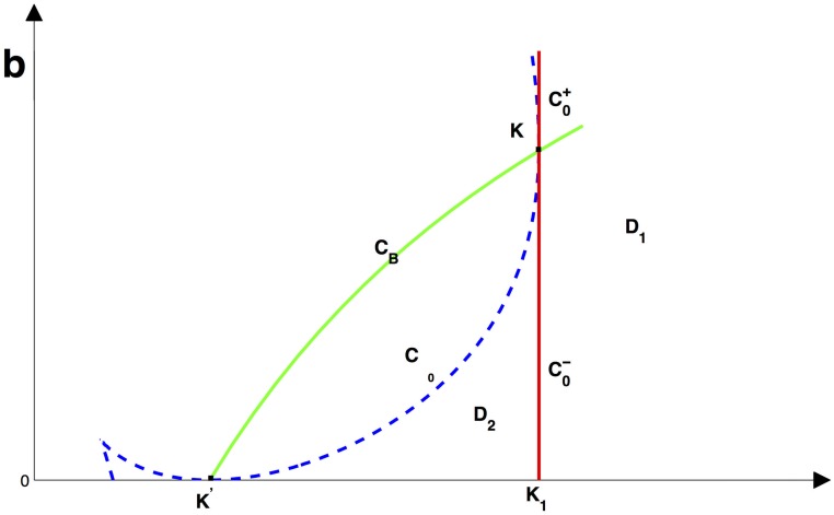
Based on the above analysis, we know that system (5) undergoes some bifurcation. In order to consider the impact of hospital bed number and the incidence rate on the dynamics of the model, we will chose b and β as bifurcation parameters to describe these bifurcations. The basic production number ${\mathbb{R}}_0=1$ defines a straight line C₀ in the (β, b) plane,

$$C_0:\beta =\frac{d{\delta }_1}{A}.$$

$\mathcal{C}=0$ also defines one branch of the hyperbolic C_B (see Fig 3),

$$C_{\mathrm{B}}:b=f_{\mathcal{C}}\left(\beta \right)=\frac{\beta A-d{\delta }_0}{\beta {\delta }_1}.$$

Fig 3. The bifurcation curves in (β, b) for system (5) when a ≠ 0.

The branch of C_B intersects with C₀ at the point $K(\frac{d{\delta }_1}{A},\frac{A({\mu }_1-{\mu }_0)}{{\delta }_1^2})$ and with β—axis at the point $K^{{}^{\prime }}(\frac{d{\delta }_0}{A},0)$. It is easily found that $f_{\mathcal{C}}$ is an increasing convex function of β in the first quadrant. Let

$$\begin{array}{c}\hfill \begin{array}{cc}& C_0^{+}=\left\{(\beta ,b)\right|\beta =\frac{d{\delta }_1}{A},b>\frac{A({\mu }_1-{\mu }_0)}{{\delta }_1^2}\},\hfill \\ & C_0^{-}=\left\{(\beta ,b)\right|\beta =\frac{d{\delta }_1}{A},b<\frac{A({\mu }_1-{\mu }_0)}{{\delta }_1^2}\},\hfill \end{array}\end{array}$$

then $C_0=C_0^{+}\cup C_0^{-}\cup K$. Here $C_0^{+}$ and $C_0^{-}$ are two branches of C₀ joint at point K.

Define the curve Δ₀(β, b) = 0 as $C_{{\Delta }_0}$, one can verify that

$$\begin{array}{ccc}& {\Delta }_0\left(K^{{}^{\prime }}\right)=0,\hfill & {\Delta }_0\left(K\right)=0,\hfill \\ & \frac{\partial b}{\partial \beta }{|}_{K^{{}^{\prime }}}=0,\hfill & \frac{\partial b}{\partial \beta }{|}_K=\pm \infty .\hfill \end{array}$$

Hence, the curve $C_{{\Delta }_0}$ is tangent to the curve C₀ at the point K and the β—axis at the point K′ when $\frac{d{\delta }_0}{A}<\beta <\frac{d{\delta }_1}{A}$.

If $\beta =\frac{d{\delta }_1}{A}$,

$$\begin{array}{c}\hfill {\Delta }_0(\beta ,b)={\Delta }_0\left(b\right)=-\frac{3d^4{(b{\delta }_1^2+A({\delta }_0-{\delta }_1))}^{2}g\left(b\right)}{A^4},\end{array}$$

where

$$\begin{array}{c}\hfill g\left(b\right)=A^2{a}^2{\delta }_1^2{b}^2-2Aa{\delta }_0{\delta }_1^{2}b-{\delta }_0(4A^{2}a({\delta }_0-{\delta }_1)-{\delta }_0{\delta }_1^2).\end{array}$$

Denote the discrimination of g(b) = 0 as ${\Delta }_2=16A^4{a}^3{\delta }_1^2{\delta }_0({\delta }_0-{\delta }_1)<0$. Hence the equation Δ₀(b) = 0 has a unique real solution, $b=\frac{A({\mu }_1-{\mu }_0)}{{\delta }_1^2}$, which means that K is the only point at which the curve $C_{{\Delta }_0}$ is tangent to the curve C₀.

If b = 0,

$$\begin{array}{c}\hfill {\Delta }_0(\beta ,0)={\Delta }_0\left(\beta \right)=-3{\delta }_0{(d{\delta }_0-\beta A)}^2{g}_1\left(\beta \right),\end{array}$$

where

$$\begin{array}{c}\hfill g_1\left(\beta \right)={\delta }_0{\beta }^2+4Aad\beta -4a{\delta }_0{d}^2.\end{array}$$

Through computing, we find that equation Δ₀(β, 0) = 0 has three real solutions

$$\begin{array}{c}\hfill {\beta }_0=\frac{d{\delta }_0}{A},{\beta }_{1,2}=\frac{-2adA\pm 2d\sqrt{A^2{a}^2+a{\delta }_0^2}}{{\delta }_0}.\end{array}$$

It is easy to verify β₀ > β₁, so the curve $C_{{\Delta }_0}$ will not intersect with the abscissa axis when $\beta \in (\frac{d{\delta }_0}{A},\frac{d{\delta }_1}{A}]$.

For the curve C_B, note

$$\begin{array}{c}\hfill \begin{array}{ccc}{\Delta }_0(\beta ,\frac{\beta A-d{\delta }_0}{\beta {\delta }_1})\hfill & =\hfill & {\displaystyle \frac{12{(ad(\beta A-d{\delta }_0)/\beta +\beta {\delta }_0)}^3(\beta A-d{\delta }_0)(d{\delta }_1-\beta A)}{\beta {\delta }_1}}\hfill \\ & & +{\displaystyle \frac{81a^2{d}^2{\delta }_0^2{(\beta A-d{\delta }_0)}^2{(d{\delta }_1-\beta A)}^2}{{\beta }^2{\delta }_1^2}}.\hfill \end{array}\end{array}$$ (35)

Obviously, if $\beta \in (\frac{d{\delta }_0}{A},\frac{d{\delta }_1}{A}]$, then ${\Delta }_0(\beta ,\frac{\beta A-d{\delta }_0}{\beta {\delta }_1})>0$. Hence, the curve C_B is located above the curve $C_{{\Delta }_0}$ for $\beta \in (\frac{d{\delta }_0}{A},\frac{d{\delta }_1}{A}]$.

Based on the above the discussion and Theorem 0.1, if we define

$$\begin{array}{c}\hfill \begin{array}{c}{D}_1=\left\{(\beta ,b)\right|\beta >\frac{d{\delta }_1}{A},b>0\},\hfill \\ D_2=\left\{(\beta ,b)\right|\frac{d{\delta }_0}{A}<\beta <\frac{d{\delta }_1}{A},0<b<\frac{A({\mu }_1-{\mu }_0)}{{\delta }_1^2},{\Delta }_0(\beta ,b)<0\},\hfill \end{array}\end{array}$$

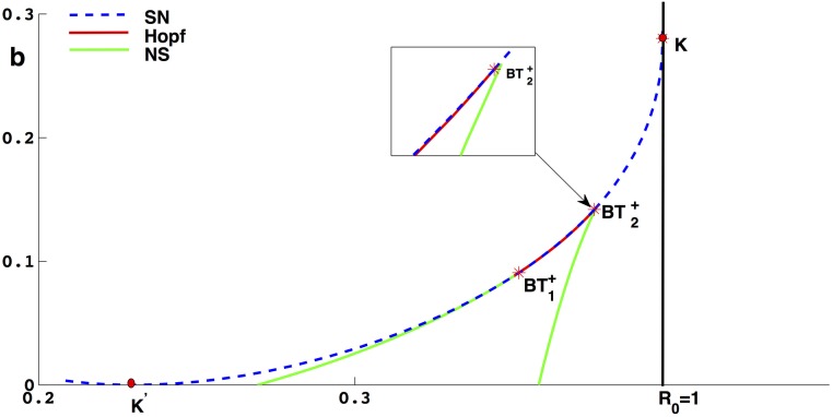
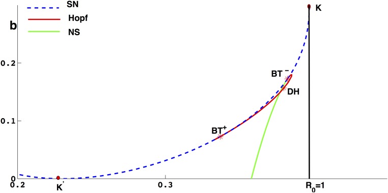
then there is one endemic equilibria in the region D₁ and two endemic equilibria in the region D₂. System (5) undergoes saddle-node bifurcation on the cure $C_{{\Delta }_0}$ when $\beta \in (\frac{d{\delta }_0}{A},\frac{d{\delta }_1}{A}]$. The backward bifurcation occurs on the $C_0^{-}$ and forward bifurcation occurs on the $C_0^{+}$. The pitchfork bifurcation occurs when transversally passing through the curve C₀ at the point K. Especially, if a = 0, system (5) has a semi-hyperbolic node of codimension 2 at the point K and we can solve b in term of β from Δ₀(β, b) = 0,

$$\begin{array}{c}\hfill b=f_{\Delta }^{\pm }\left(\beta \right)=\frac{\beta A({\delta }_1-{\delta }_0)+{\delta }_0(d{\delta }_1-\beta A)\pm 2\sqrt{\beta A{\delta }_0({\delta }_1-{\delta }_0)(d{\delta }_1-\beta A)}}{\beta {\delta }_1^2}.\end{array}$$ (36)

Now, we discuss the Hopf bifurcation of system (5). It follows from Eq (18) that if Hopf bifurcation occurs at one endimic equilibrium $E(\overline{S},\overline{I})$, we have tr(J_E) = 0. Note that from Eq (19) we can rewrite tr(J_E) as

$$\text{tr}\left(J_E\right)=-\frac{h_1\left(\overline{I}\right)}{{(b+\overline{I})}^2{(1+a{\overline{I}}^2)}^2},$$

where

$$\begin{array}{c}\hfill h_1\left(\overline{I}\right)=b_4{\overline{I}}^4+b_3{\overline{I}}^3+b_2{\overline{I}}^2+b_1\overline{I}+b^{2}d,\end{array}$$ (37)

with

$$\begin{array}{c}\hfill \begin{array}{c}{b}_4=a(3d+2{\mu }_0+2\alpha ),\hfill \\ b_3=a(6bd+3b{\mu }_0+b{\mu }_1+4b\alpha )+\beta ,\hfill \\ b_2=a(3b^{2}d+2b^2{\mu }_1+2b^2\alpha )+2b\beta +d,\hfill \\ b_1=b(b\beta +2d+{\mu }_0-{\mu }_1).\hfill \end{array}\end{array}$$

Here, $h_1\left(\overline{I}\right)$ is a quartic equation. Since b₂, b₃ and b₄ are non-negative, if $b>\frac{{\mu }_1-{\mu }_0-2d}{\beta }$, h₁(I) > 0, in order to make sure that h₁(I) = 0 has a positive root, we must have $b<\frac{{\mu }_1-{\mu }_0-2d}{\beta }$. This means sufficient number of hospital beds excludes the possibility of the disease oscillation. From the expression of $h_1\left(\overline{I}\right)$ in Eq (37), it is not an easy task to study the Hopf bifurcation from the polynomial Eq (37), we will study a simple case when a = 0, and give the simulations to explore the case when a is small.

When a = 0, the polynomial Eq (37) is reduced to

$$h_1\left(\overline{I}\right)=\beta {\overline{I}}^3+(d+2b\beta ){\overline{I}}^2+b_1\overline{I}+b^{2}d.$$

One can verify the following lemma

Lemma 0.8. For any positive equilibrium, if $b\ge \frac{{\mu }_1-{\mu }_0-2d}{\beta }$, we alway have tr(J_E)<0.

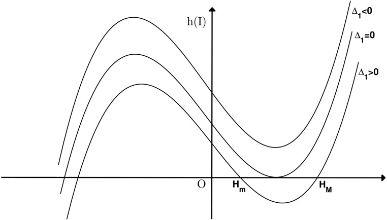
In order to study Hopf bifurcation and Bogdanov-Takens bifurcation, we will assume that $b<\frac{{\mu }_1-{\mu }_0-2d}{\beta }$. Denote the discrimination of $h_1\left(\overline{I}\right)$ as Δ₁. Since b₁ < 0, function $h_1\left(\overline{I}\right)$ must have one negative real root. As shown in Fig 4, It is not difficult to verify function $h_1\left(\overline{I}\right)$ has two humps which locate on the different sides of vertical axis, and the maximum is obtained on the left hump, while the minimum is obtained on the right hump.

Fig 4. Graph of h(I) with different signs of Δ₁ when b₁ < 0.

When I₂ = H_m, I₂ = H_M or I₂ = H_M = H_m, Hopf bifurcation occurs. BT bifurcation of codimension 2 occurs when I* = H_m or I* = H_M and BT bifurcation of codimension 3 occurs when I* = H_m = H_M.

The number of roots of function $h_1\left(\overline{I}\right)$ is determined by the sign of the Δ₁. When exist, we denote the roots as H_m and H_M with H_M ≥ H_m.

Lemma 0.9. $\frac{\partial I_2}{\partial \beta }>0,\forall \beta >0and\frac{\partial I_2}{\partial b}<0,\forall b>0$.

Proof. From the Eq (9) and the expression of I₂, direct calculation leads to

$$\begin{array}{c}{\displaystyle \frac{\partial I_2}{\partial \beta }}=-{\displaystyle \frac{\partial f}{\partial \beta }}/{\displaystyle \frac{\partial f}{\partial I_2}}={\displaystyle \frac{d{\delta }_{0}I+bd{\delta }_1}{\beta \sqrt{\Delta }}}>0,\hfill \\ {\displaystyle \frac{\partial I_2}{\partial b}}={\displaystyle \frac{1}{2\mathcal{B}}}\left[-{\displaystyle \frac{\partial \mathcal{C}}{\partial b}}+{\displaystyle \frac{1}{\sqrt{\Delta }}}(\mathcal{C}{\displaystyle \frac{\partial \mathcal{C}}{\partial b}}-2\mathcal{B}{\displaystyle \frac{\partial \mathcal{D}}{\partial b}})\right].\hfill \end{array}$$

One can find that $\frac{\partial \mathcal{C}}{\partial b}=\beta {\delta }_1>0$. We will prove ${\displaystyle \frac{\partial I_2}{\partial b}}<0$ in two cases. If ${\mathbb{R}}_0<1$, then $\frac{\partial \mathcal{D}}{\partial b}=d{\delta }_1-\beta A>0$. Recall the analysis of the existence of the equilibria we know that the $\mathcal{C}<0$, so the $\frac{\partial I_2}{\partial b}<0$. If ${\mathbb{R}}_0>1$, then ${lim}_{b\to +\infty }\frac{\partial I_2}{\partial b}=0$ and

$$\begin{array}{cc}{\displaystyle \frac{\partial I_2^2}{{\partial }^{2}b}}\hfill & =-{\displaystyle \frac{{\Delta }_0^{-3/2}}{8\mathcal{B}}}\left[{\left({\displaystyle \frac{\partial {\Delta }_0}{\partial b}}\right)}^2-2{\Delta }_0{\displaystyle \frac{{\partial }^2{\Delta }_0}{{\partial }^{2}b}}\right]\hfill \\ & =2{\beta }^{2}A({\mu }_1-{\mu }_0)(\beta A-d{\delta }_1)>0,\hfill \end{array}$$

so the ${\displaystyle \frac{\partial I_2\left(b\right)}{\partial b}}$ is an increasing function of b with supremum 0 in the (0, +∞), so for ∀b > 0 $\frac{\partial I_2\left(b\right)}{\partial b}<0$.

Theorem 0.10. For system (5) with a = 0, generic Hopf bifurcation could occur if I₂ = H_m, I₂ = H_M or I₂ = H_m = H_M.

Proof. We only need to verify the transversality condition. Let γ = tr(I₂)/2 be the real part of the two solutions of Eq (18), when a = 0.

If I₂ = H_M or I₂ = H_M = H_m, we consider β as the bifurcation parameter and fix all other parameters. Then

$$\begin{array}{cc}\hfill {\displaystyle \frac{d\gamma }{d\beta }}{|}_{\beta =\widehat{\beta }}=& {\displaystyle \frac{1}{2}}\left[{\displaystyle \frac{\partial \text{tr}(I_2\left(\beta \right),\beta )}{\partial I_2}}{\displaystyle \frac{\partial I_2\left(\beta \right)}{\partial \beta }}+{\displaystyle \frac{\partial \text{tr}(I_2\left(\beta \right),\beta )}{\partial \beta }}\right]{|}_{\beta =\widehat{\beta }},\hfill \\ \hfill {\displaystyle \frac{\partial \text{tr}(I_2\left(\beta \right),\beta )}{\partial I_2}}{|}_{\beta =\widehat{\beta }}=& -{\displaystyle \frac{2h^{{}^{\prime }}\left(H_M\right)}{{(b+H_M)}^2}}<0,\hfill \\ \hfill {\displaystyle \frac{\partial \text{tr}(I_2\left(\beta \right),\beta )}{\partial \beta }}{|}_{\beta =\widehat{\beta }}=& -{\displaystyle \frac{H_M^3+2b{H}_M^2+b^2{H}_M}{{(b+H_M)}^2}}<0.\hfill \end{array}$$

From Lemma 0.9, we have $\frac{\partial I_2}{\partial \beta }{|}_{\beta =\widehat{\beta }}>0$, so $\frac{d\gamma }{d\beta }<0$.

If I₂ = H_m or I₂ = H_M = H_m, we consider b as the bifurcation parameter and fix all the other parameters. Then

$$\begin{array}{cc}\hfill {\displaystyle \frac{d\gamma }{db}}{|}_{b=\widehat{b}}=& {\displaystyle \frac{1}{2}}\left[{\displaystyle \frac{\partial \text{tr}(I_2\left(b\right),b)}{\partial I_2}}{\displaystyle \frac{\partial I_2\left(b\right)}{\partial b}}+{\displaystyle \frac{\partial \text{tr}(I_2\left(b\right),b)}{\partial b}}\right]{|}_{b=\widehat{b}},\hfill \\ \hfill {\displaystyle \frac{\partial \text{tr}(I_2\left(b\right),b)}{\partial b}}{|}_{b=\widehat{b}}=& -{\displaystyle \frac{2h^{{}^{\prime }}\left(H_m\right)}{{(b+H_m)}^2}}>0,\hfill \\ \hfill {\displaystyle \frac{\partial \text{tr}(I_2\left(b\right),b)}{\partial b}}{|}_{b=\widehat{b}}=& {\displaystyle \frac{(b-H_m)({\mu }_0-{\mu }_1)}{{(b+H_m)}^2}}<0.\hfill \end{array}$$

From Lemma 0.9, we have $\frac{\partial I_2}{\partial b}{|}_{b=\widehat{b}}<0$, so $\frac{d\gamma }{d{\mu }_1}<0$ (one can verify that H_m < b). Then the proof of theorem is completed.

The reason why we choose different parameters to unfold Hopf bifurcation in Theorem 0.10 is that the transversality condition may fail at some point if we focus on one parameter.

In order to verify that Hopf bifurcation occurs in the system, we need to know the type of E₂. If E₂ is a weak focus, Hopf bifurcation can happen, otherwise system does not undergo Hopf bifurcation. Because system (5) is analytic when a = 0, E₂ can only be weak focus or center. We can distinguish these two types of singularities by calculating Lyapunov coefficients and verifying it through numerical simulation.

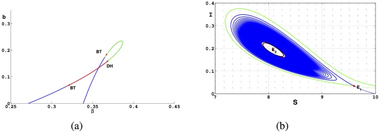
Taking the resultant of f(I) and $h_1\left(\overline{I}\right)$ with respect to I, we can get the curve q(β, b) in the space (β, b), and plot the algebraic curve q(β, b) = 0 by fixing other parameters A, d, μ₁, α and μ₀. Choose A = 3, d = 0.3, α = 0.5, μ₀ = 1.5, μ₁ = 3 and plot q(β, b) = 0 in the plane (β, b) as shown in Fig 5(a). The green curve (δ₁ < 0) represents supercritical Hopf bifurcation; the red curve corresponding to δ₁ > 0 represents subcritical Hopf bifurcation.

Fig 5. Graphs of Bifurcation curve in parameters plane (β, b) and the phase trajectory for system (5).

(a) Curve q(β, b) = 0. The green curve is supercritical Hopf bifurcation; The red curve is subcritical Hopf bifurcation. σ₁ becomes 0 at the DH point. (b) Two limit cycles bifurcation from the weak focus E₂.

We choose a point(β, b) = (0.3683, 0.1587) in Fig 5(a) to plot the phase portrait at the point. In Fig 5(b), as t → +∞, the trajectory starting at (9, 0.1) spirals outward to the stable limit cycle (red curve) and E₂(8.0794, 0.19363) is stable. Because system (5) is a plane system, there must exist a unstable limit cycle between the stable endemic equilibria and stable limit cycle (black curve). The blue curve in the Fig 5(b) is the unstable manifold of E₁.

Bogdanov-Takens bifurcation

From Theorem 0.1 we know that the two equilibria E₁ and E₂ coalesce at the equilibria E*(S*, I*) when ${\mathbb{R}}_0={\mathbb{R}}_0^c$, if a = 0, where

$$\begin{array}{c}{S}^{*}={\displaystyle \frac{A}{d+\beta I^{*}}},\hfill \\ I^{*}=-{\displaystyle \frac{d(d+\alpha +{\mu }_0)-\beta A+b\beta (d+\alpha +{\mu }_1)}{2\beta (d+\alpha +{\mu }_0)}}.\hfill \end{array}$$

We can find that det(I*) = 0 in Eq (18) if ${\mathbb{R}}_0={\mathbb{R}}_0^c$. From Proposition 0.7, we know that E* is a saddle-node point if tr(I*) ≠ 0. If tr(I*) = 0, Eq (18) has a zero eigenvalue with multiplicity 2, which suggests that system (5) may admit a Bogdanov-Takens bifurcation. Then, we give the following theorem.

Theorem 0.11. For system (5) with a = 0, suppose that Δ = 0, h(I*) = 0 and h′(I*) ≠ 0, then E* is a Bogdanov-Takens point of codimension 2, and system (5) localized at E* is topologically equivalent to

$$\begin{array}{c}\hfill \left\{\begin{array}{c}\dot{X}=Y,\hfill \\ \dot{Y}=X^2+Sign\left(h^{{}^{\prime }}\left(I^{*}\right)\right)XY+{O\left(\right|X,Y|}^3).\hfill \end{array}\right.\end{array}$$ (38)

Proof. Changing the variables as x = S − S*, y = I − I*, then system (5) becomes

$$\begin{array}{c}\hfill \left\{\begin{array}{c}{\displaystyle \frac{dx}{dt}}=-(d+\beta I^{*})x-\beta S^{*}y-\beta xy,\hfill \\ {\displaystyle \frac{dy}{dt}}=\beta I^{*}x+{\displaystyle \frac{({\mu }_1-{\mu }_0)b{I}^{*}}{{(b+I^{*})}^2}}y+C{y}^2+\beta xy+{O\left(\right|x,y|}^3),\hfill \end{array}\right.\end{array}$$ (39)

where

$$\begin{array}{c}\hfill C={\displaystyle \frac{({\mu }_1-{\mu }_0)b}{{(b+I^{*})}^2}}-{\displaystyle \frac{({\mu }_1-{\mu }_0)b{I}^{*}}{{(b+I^{*})}^3}}.\end{array}$$ (40)

tr(I*) = 0 and det(I*) = 0 imply that

$$\begin{array}{c}\hfill \begin{array}{cc}{\beta }^2{S}^{*}{I}^{*}-{(d+\beta I^{*})}^2=0,\hfill & d+\beta I^{*}=\frac{({\mu }_1-{\mu }_0)b{I}^{*}}{{(b+I^{*})}^2},\hfill \end{array}\end{array}$$ (41)

so the generalized eigenvectors corresponding to λ = 0 of Jacobian matrix in system (5) at the point E* are

$$\begin{array}{c}\hfill \begin{array}{cc}{V}_1={(-d-\beta I^{*},\beta I^{*})}^{{}^{\prime }},\hfill & V_2={(1,0)}^{{}^{\prime }}.\hfill \end{array}\end{array}$$ (42)

Let T = (T_ij)_2×2 = (V₁, V₂), then under the non-singular linear transformation

$$\begin{array}{c}\hfill \left(\begin{array}{c}x\\ y\end{array}\right)=T\left(\begin{array}{c}X\\ Y\end{array}\right),\end{array}$$

where |T| = −βI* < 0. System (39) becomes

$$\begin{array}{c}\hfill \left\{\begin{array}{c}\dot{X}=Y+a_{11}{X}^2+\beta XY,\hfill \\ \dot{Y}=a_{21}{X}^2+d\beta XY+{O\left(\right|X,Y|}^3),\hfill \end{array}\right.\end{array}$$ (43)

here

$$\begin{array}{c}\hfill \begin{array}{c}{a}_{11}=-{\displaystyle \frac{(d+\beta I^{*}){\beta }^2{I}^{*}-\left(\frac{({\mu }_1-{\mu }_0)b}{{(b+I^{*})}^2}-\frac{({\mu }_1-{\mu }_0)b{I}^{*}}{{(b+I^{*})}^3}\right){\beta }^2{I}^{{*}^2}}{\beta I^{*}}},\hfill \\ a_{21}={\displaystyle \frac{\beta I^{*}(\beta I^{*}+d)(b\beta -d)}{b+I^{*}}}.\hfill \end{array}\end{array}$$

Using the near-identity transformation

$$\begin{array}{c}\hfill u=X-\frac{a_{12}{X}^2}{2},v=Y+a_{11}{X}^2,\end{array}$$ (44)

and rewrite u, v into X, Y, we obtain

$$\begin{array}{c}\hfill \left\{\begin{array}{c}\dot{X}=Y+{O\left(\right|X,Y|}^3),\hfill \\ \dot{Y}=M_{21}{X}^2+M_{22}XY+{O\left(\right|X,Y|}^3).\hfill \end{array}\right.\end{array}$$ (45)

To consider the sign of M₂₁, note that

$$M_{21}=a_{21}={\displaystyle \frac{\beta I^{*}(\beta I^{*}+d)(b\beta -d)}{b+I^{*}}}.$$

For system (5), the condition of the existence of endemic equilibrium is $b<\frac{d({\mu }_1-{\mu }_0)}{\beta {\delta }_1}$, hence, M₂₁ < 0. Then we will determine the sign of M₂₂ by

$$\begin{array}{ll}{M}_{22}\hfill & =a_{22}+2a_{11}\hfill \\ \hfill & =d\beta -2\frac{\left(d+\beta I^{*}\right){\beta }^2{I}^{*}-\left(\frac{\left({\mu }_1-{\mu }_0\right)b}{{\left(b+I^{*}\right)}^2}-\frac{\left({\mu }_1-{\mu }_0\right)b{I}^{*}}{{\left(b+I^{*}\right)}^3}\right){\beta }^2{I}^{{*}^2}}{\beta I^{*}}\hfill \\ \hfill & =-\frac{\beta h^{{}^{\prime }}\left(I^{*}\right)}{{\left(b+I^{*}\right)}^2}.\hfill \end{array}$$

If h′(I*) ≠ 0, we make a change of coordinates and time and preserve the orientation by time

$$\begin{array}{c}\hfill X\to \frac{M_{21}}{a_{22}^2}X,Y\to \frac{M_{21}^2}{a_{22}^3}Y,t\to \left|\frac{a_{22}}{M_{21}}\right|t\end{array}$$ (46)

then system (5) is topologically equivalent to the normal form Eq (38).

From Theorem 0.11, we know that if a = 0, endemic equilibrium E* is a Bogdanov-Takens point of codimension 2 when Δ = 0, h(I*) = 0 and h′(I*) ≠ 0. If h′(I*) = 0, E* may be a cusp of codimension 3.

In [28], a generic unfolding with the parameters ε = (ε₁, ε₂, ε₃) of the codimension 3 cusp singularity is C^∞ equivalent to

$$\begin{array}{c}\hfill \left\{\begin{array}{c}\dot{X}=Y,\hfill \\ \dot{Y}={\epsilon }_1+{\epsilon }_{2}Y+{\epsilon }_{3}XY+X^2-X^{3}Y+{O\left(\right|X,Y|}^4).\hfill \end{array}\right.\end{array}$$ (47)

About system (47), we can find that the system has no equilibrium if ε₁ > 0. The plane ε₁ = 0 excluding the origin in the parameter space is saddle-node bifurcation surface. When ε₁ decrease from this surface, the saddle-node point of Eq (47) becomes a saddle and a node. Then the other bifurcation surfaces are situated in the half space ε₁ < 0. They can be visualized by drawing their trace on the half-sphere

$$\begin{array}{c}\hfill S=\left\{({\epsilon }_1,{\epsilon }_2,{\epsilon }_3)\right|{\epsilon }_1<0,{\epsilon }_1^2+{\epsilon }_2^2+{\epsilon }_3^2={\sigma }^2\},\end{array}$$ (48)

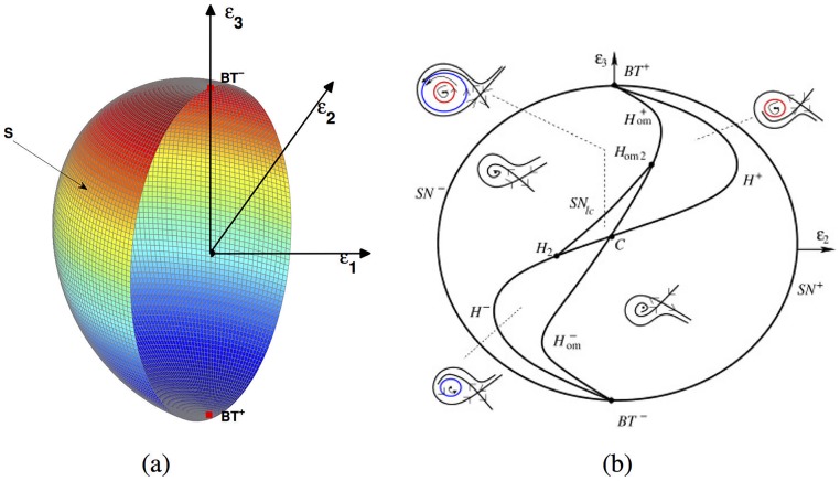
when σ > 0 sufficiently small (see Fig 6(a)). We recall that the bifurcation set is a ‘cone’ based on its trace with S.

Fig 6. The bifurcation diagram of BT of codimension 3.

(a) The parameter space and the trace of the bifurcation diagram on the S(ϵ₁ ≤ 0); (b) The sign of the BT is positive if the coefficient of the term XY in the norm form is positive, otherwise it is negative [24].

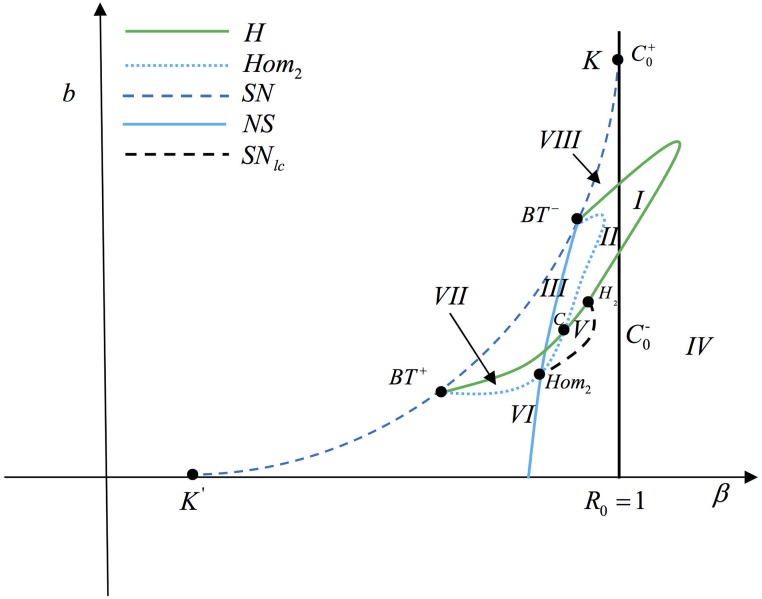
In Fig 6(b), trace on the S which consists of 3 curves: a curve H_om of homoclinic bifurcation, a H of Hopf bifurcation and SN_lc of double limit cycle bifurcation. The curve SN_lc include two points H₂ and H_om2 and the curve SN_lc tangent to the curves H and H_om. The curves H and H_om touch the $\partial S=\left\{({\epsilon }_1,{\epsilon }_2,{\epsilon }_3)\right|{\epsilon }_1=0,{\epsilon }_2^2+{\epsilon }_3^2={\sigma }^2\}$ with a first-order tangency at the points BT⁺ and BT⁻. In the neighbourhood of the BT⁺ and BT⁻, one can find the unfolding of the cusp-singularity of codimension 2. For system (47), there exists an unstable limit cycle between H and H_om near the BT⁺ and an unique stable limit cycle between H and H_om near the BT⁻. In the curved triangle CH₂H_om2 the system has two limit cycles, the inner one unstable and the outer one stable. These two limit cycles coalesce when the ε crosses over the curve SN_lc. On the SN_lc there exists a unique semistable limit cycle. The more interpretation can be found in literature [24, 28].

Bifurcation diagram and simulation

According to analysis and Theorem 0.11, we know that system (5) undergoes Bogdanov-Takens bifurcation of codimension 2. In this section we will choose the parameters β and b as bifurcation parameters to present the bifurcation diagram by simulations. In the proof of Theorem 0.11, we make a series of changes of variables and time, so there will be different situations with different signs of h′(I). According to the positive and negative coefficients of XY term in the normal form Eq (47), we denote the Bogdanov-Takens bifurcation of codimension 2 as BT⁺ and BT⁻ respectively.

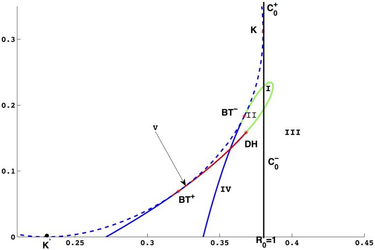
Taking A = 3, d = 0.3, α = 0.5, μ₀ = 1.5, μ₁ = 3, a = 0, we find that (β, b) = (0.367004, 0.183323) satisfying the conditions in Theorem 0.11, then we use (β, b) to unfold the Bogdanov-Takens bifurcation of codimension 2. By simulation, we obtain the bifurcation diagram in plane (β, b) shown as Fig 7, the blue dash (solid) curve represents saddle-node bifurcation (neutral saddle), the green (blue solid) curve represents supercritical (subcritical) Hopf bifurcation and the parameter space (β, b) is divided into differen areas by these bifurcation curves. There are two Bogdanov-Takens bifurcation points, BT⁻(0.367004, 0.183323) and BT⁺(0.321298, 0.069049). In order to distinguish these two points, we get some phase diagrams of system when β and b located in different area of (β, b) shown as Fig 8.

Fig 7. The bifurcation diagram in plane (β, b).

There are two types of Bogdanov-Takens bifurcation, BT⁺ and BT⁻. The green curve represents supercritical Hopf bifurcation, the red curve represents subcritical Hopf bifurcation. The blue dash (solid) curve represents saddle-node bifurcation (neutral saddle curve).

Fig 8. The phase diagram of system (5).

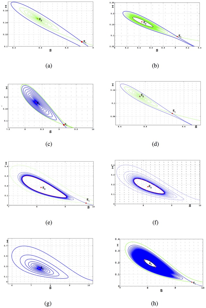
The blue curve represents unstable manifold, green curve represents stable manifold. (a) b = 0.1, β = 0.339; (b) b = 0.1, β = 0.340; (c) b = 0.1, β = 0.3415; (d) b = 0.18, β = 0.367; (e) b = 0.18, β = 0.3737; (f) b = 0.21, β = 0.3815; (g) b = 0.21, β = 0.4; (h) b = 0.1587, β = 0.3683. In the (b), there is an unstable limit cycle marked black curve near the epidemic equilibrium E₂. In the (e) and (f), there is a stable limit cycle marked red curve. In the (h), we find that there are two limit cycle, the small one is unstable, the another one is stable.

In Fig 8(a), β, b are located in the area between saddle-node bifurcation and subcritical Hopf bifurcation curve and the epidemic equilibrium E₂ is a unstable focus. In the IV, the phase diagram of system is one of the cases shown as (b), (c) and (h). There is an unstable limit cycle (black curve) near the epidemic equilibrium E₂ in Fig 8(b) and two limit cycles in Fig 8(h) with the inner one unstable and the other one stable. When β and b are located in II, the phase diagram of system is one of the cases as shown in (d) and (e) and there is a stable limit cycle in Fig 8(e). When β and b are located in I or III, the phase portraits are similar to the cases of (f) and (g), respectively. In the case (f), system (5) has a unique epidemic equilibrium and a stable limit cycle.

In the small neighborhood of BT⁺, we know that the unstable limit cycle bifurcating from Hopf bifurcation curve disappears from the homoclinic loop, and from Fig 8(b) and 8(c), we can observe that the homoclinic loops are located in IV. Otherwise, from Fig 8(d) and 8(e), we can obtain that the homoclinic loops are located in II which is in the small neighborhood of BT⁻. Hence, the Hopf bifurcation curve and homoclinic loops switch their positions at some point C. In order to figure out the relative positions of C, H₂ and Hom₂, as shown in Fig 9 we change the value of β and plot the bifurcation diagram on (β, b) with different b.

Fig 9. Bifurcation diagram in (β, I) with different b.

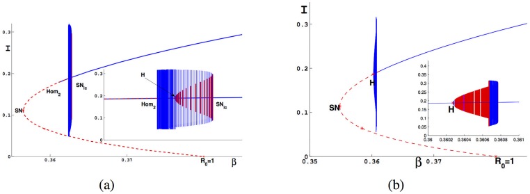
The red dash(solid) represents unstable epidemic equilibrium(limit cycle). The blue curve represents stable epidemic equilibrium or limit cycle. (a) b = 0.145; (b) b = 0.14.

By simulations, we get the case (a) and (b) in Fig 9, we now know that two limit cycles bifurcating from the semi-stable cycle with one disappearing from the Homoclinic loop and the another disappearing from the Hopf bifurcation curve. We therefore obtain $b_{H_2}>b_C>b_{H_{om2}}$ by the order these two limit cycle vanishing with different values of b.

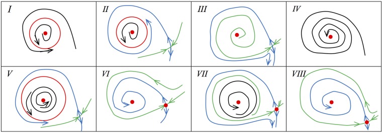
Then we obtain the bifurcation diagrams of system (5) near the Bogdanov-Takens bifurcation and the phase portraits in some regions of parameters shown as Figs 10 and 11 respectively.

Fig 10. Bifurcation digram near the Bogdanov-Takens.

Fig 11. Phase portraits for parameters in different regions of Fig 10.

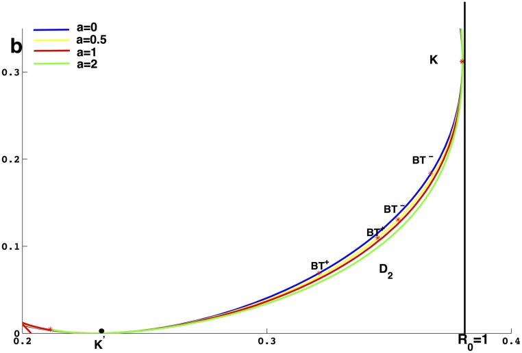
From the above dynamical analysis, we know that system (5) has complex dynamic behavior even though a = 0. For system (5), we also find the same phenomenon by the simulation as shown in the Fig 12 for the case a ≠ 0. In the simulation, the parameters excluding a are the same as the simulation setting. From Fig 12, we find that the region D₂ and the distance between BT⁺ and BT⁻ becomes small when a becomes lager, which means that choosing a as one other bifurcation parameter can unfold the system (5) and system (5) may undergo the Bogdanov-Takens bifurcation of codimension 3.

Fig 12. The curve q(β, b) = 0 with different values of a.

The blue curve, yellow curve, red curve and green curve are drawn according to a = 0, a = 0.5, a = 1 and a = 2 respectively.

Discussion and application

In this paper we consider the SIR model with the nonmonotone incidence rate due to the intervention strategies and nonlinear recovery rate considering the hospitalization conditions.

From Theorem 0.1, we know that system (4) undergoes backward bifurcation. In Theorem 0.3, we get the necessary and sufficient condition of backward bifurcation is $b<\frac{A({\mu }_1-{\mu }_0)}{{\delta }_1^2}$ when ${\mathbb{R}}_0=1$, which means that we can eliminate the disease if $b>\frac{A({\mu }_1-{\mu }_0)}{{\delta }_1^2}$ and $\beta <\frac{d{\delta }_1}{A}$ i.e we need enough number of hospital beds. From the Lemma 0.8, we know that if $b>\frac{{\mu }_1-{\mu }_0-2d}{\beta }$, system (5) will not have periodic solution, and the endemic equilibrium E₂ is stable. We then discuss Hopf bifurcation and BT bifurcation for system (5) and present in details about these bifurcations in the case a = 0 and present the bifurcation diagrams in Figs 8 and 10.

From the discussion we get Lemma 0.9, which implies that I₂(b) is a monotone decreasing function of b. Hence, increasing the number of beds can only reduce the number of the total infected individuals, but can not eliminate the diseases as shown in Fig 13(a) if ${\mathbb{R}}_0>1$. If ${\mathbb{R}}_0<1$, from Fig 3 and Eq (36), we know that if $b>b_c=f_{\Delta }^{-}$ we can eliminate the disease, and these rich dynamics finally disappear through the saddle-node bifurcation when b = b_c as shown in Figs 7 and 13(b) and 13(c).

Fig 13. Bifurcation in the plane (b, I) with different μ₁.

β = 0.39, a = 0. (a) ${\mathbb{R}}_0=1.02$; (b) ${\mathbb{R}}_0=0.98$; (c) ${\mathbb{R}}_0=0.95$.

For system (3) with a ≠ 0, taking A = 3, d = 0.3, β = 0.5, a = 0.2, μ₁ = 3.1728627 and μ₀ = 1.5 we get the bifurcation diagram with different values for c as shown as Figs 14 and 15. In Fig 14, the types of BT-bifurcation are the same, however, there are two types of BT bifurcations in the Fig 15.

Fig 14. The bifurcation diagram of system (3) in parameters plane (β, b).

A = 3, d = 0.3, β = 0.5, c = 0.185, a = 0.2, μ₁ = 3.1728627, μ₀ = 1.5, $B{T}_1^{+}(0.353073,0.0925301),$ $B{T}_2^{+}(0.375,0.137406)$.

Fig 15. The bifurcation diagram of system (3) in parameters plane (β, b).

A = 3, d = 0.3, β = 0.5, c = 0.1, a = 0.2, μ₁ = 3.1728627, μ₀ = 1.5, BT⁺(0.337066, 0.072821), BT⁻(0.382572, 0.172627).

In Fig 16, A = 3, β = 0.375, α = 0.5, μ₀ = 0.5 we plot the phase portraits in plane (S, I) with different d, in these cases $\frac{\beta A}{d(d+\alpha +{\mu }_0)}<1$, and find that there is an unstable limit cycle near the E₂ when d = 1.483783. From the above stimulation, we know that Therorem 0.4 is not ture when $-2\sqrt{a}<c<0$.

Fig 16. Phase portraits of system (3) in the plane (S, I) with different d.

A = 3, β = 0.375, α = 0.5, μ₀ = 0.5, μ₁ = 0.7, a = 0.7, b = 0.01, c = −1.65. (a) d = 1.49; (b) d = 1.483783; (c) d = 1.4. In case (a) (b) and (c), E₁ is always a saddle and E₀ is a stable node. E₂ is a stable node in case (b) and (c), while it is a unstable node in case (a). There is an unstable limit cycle near E₂ in case (b).

According to an early SIR model with nonmonotone incidence rate in the literature [19], the dynamics of the system are completely determined by ${\mathbb{R}}_0$, which means that the disease will be eliminated if ${\mathbb{R}}_0<1$, otherwise the disease persist. Contrasting to their work and the other results for classic epidemic models, we find that the nonlinear recovery rate is also an important factor which leads to very complicated dynamics. Moreover, we find that ${\mathbb{R}}_0$ is not enough to determine the dynamic behavior in system (5). By simulations, we predict that there would exist b_1c in system (3)? which has the same role as b_c. Hopefully we can explore more relationships between the intervention actions, hospitalization conditions and spread of diseases, to provide the guidelines for public and desicion makers.

Data Availability

All relevant data are within the paper and its Supporting Information files.

Funding Statement

This work is supported by the National Science Foundation of China (11331009), Research Project Supported by Fund Program for the Scientific Activities of Selected Returned Overseas Professionals in Shanxi Province and the National Sciences Foundation of Shanxi Province (2015011009).

References

- 1.Brauer F, Castillo-Chavez C. Mathematical models in population biology and epidemiology[M]. New York: Springer, 2001. [Google Scholar]
- 2.Kermack W O, McKendrick A G. A contribution to the mathematical theory of epidemics[C] Proceedings of the Royal Society of London A: Mathematical, Physical and Engineering Sciences. The Royal Society, 1927, 115(772): 700–721. [Google Scholar]
- 3.Hethcote H W. The mathematics of infectious diseases[J]. SIAM review, 2000, 42(4): 599–653. 10.1137/S0036144500371907 [DOI] [Google Scholar]
- 4.Gumel A B, Ruan S, Day T, et al. Modelling strategies for controlling SARS outbreaks[J]. Proceedings of the Royal Society of London B: Biological Sciences, 2004, 271(1554): 2223–2232. 10.1098/rspb.2004.2800 [DOI] [PMC free article] [PubMed] [Google Scholar]
- 5.Li Li. Monthly periodic outbreak of hemorrhagic fever with renal syndrome in China[J]. Journal of Biological Systems, 2016, 24, 519–533. 10.1142/S0218339016500261 [DOI] [Google Scholar]
- 6.Li Li. Patch invasion in a spatial epidemic model[J]. Applied Mathematics and Computation, 2015, 258, 342–349. 10.1016/j.amc.2015.02.006 [DOI] [Google Scholar]
- 7.Gui-Quan Sun, et al. , Transmission dynamics of cholera: Mathematical modeling and control strategies[J]. Commun. Nonlinear Sci. Numer. Simulat., 2017, 45, 235–244. 10.1016/j.cnsns.2016.10.007 [DOI] [Google Scholar]
- 8.Ming-Tao Li, Jin Z., Sun G., Zhang J.. Modeling direct and indirect disease transmission using multi-group model[J]. J. Math. Anal. Appl., 2017, 446, 1292–1309. 10.1016/j.jmaa.2016.09.043 [DOI] [Google Scholar]
- 9.Ming-Tao Li, Sun G., Wu Y., Zhang J. and Jin Z.. Transmission dynamics of a multi-group brucellosis model with mixed cross infection in public farm[J]. Applied Mathematics and Computation, 2014, 237, 582–594. 10.1016/j.amc.2014.03.094 [DOI] [Google Scholar]
- 10.Gui-Quan Sun, Zhang Z., Global stability for a sheep brucellosis model with immigration[J], Applied Mathematics and Computation, 2014, 246, 336–345. 10.1016/j.amc.2014.08.028 [DOI] [Google Scholar]
- 11.Zhi-Qiang Xia, et al. , Modeling the transmission dynamics of Ebola virus disease in Liberia[J]. Scientific Reports, 2015, 5, 13857 10.1038/srep13857 [DOI] [PMC free article] [PubMed] [Google Scholar]
- 12.Yan-Fang Wu, Li M., Sun G.. Asymptotic analysis of schistosomiasis persistence in models with general functions[J]. Journal of the Franklin Institute, 2016, 353, 4772–4784. 10.1016/j.jfranklin.2016.09.012 [DOI] [Google Scholar]
- 13.Zhang J, Lou J, Ma Z, et al. A compartmental model for the analysis of SARS transmission patterns and outbreak control measures in China[J]. Applied Mathematics and Computation, 2005, 162(2): 909–924. 10.1016/j.amc.2003.12.131 [DOI] [PMC free article] [PubMed] [Google Scholar]
- 14.Tang S, Xiao Y, Yuan L, et al. Campus quarantine (Fengxiao) for curbing emergent infectious diseases: lessons from mitigating A/H1N1 in Xi’an, China[J]. Journal of theoretical biology, 2012, 295: 47–58. 10.1016/j.jtbi.2011.10.035 [DOI] [PubMed] [Google Scholar]
- 15.Xiao Y, Tang S, Wu J. Media impact switching surface during an infectious disease outbreak[J]. Scientific reports, 2015, 5. [DOI] [PMC free article] [PubMed] [Google Scholar]
- 16.Liu R, Wu J, Zhu H. Media/psychological impact on multiple outbreaks of emerging infectious diseases[J]. Computational and Mathematical Methods in Medicine, 2007, 8(3): 153–164. 10.1080/17486700701425870 [DOI] [Google Scholar]
- 17.Cui J, Sun Y, Zhu H. The impact of media on the control of infectious diseases[J]. Journal of Dynamics and Differential Equations, 2008, 20(1): 31–53. 10.1007/s10884-007-9075-0 [DOI] [PMC free article] [PubMed] [Google Scholar]
- 18.Cui J, Tao X, Zhu H. An SIS infection model incorporating media coverage[J]. Rocky Mountain J. Math, 2008, 38(5): 1323–1334. 10.1216/RMJ-2008-38-5-1323 [DOI] [Google Scholar]
- 19.Xiao D, Ruan S. Global analysis of an epidemic model with nonmonotone incidence rate[J]. Mathematical biosciences, 2007, 208(2): 419–429. 10.1016/j.mbs.2006.09.025 [DOI] [PMC free article] [PubMed] [Google Scholar]
- 20.Liu W, Levin S A, Iwasa Y. Influence of nonlinear incidence rates upon the behavior of SIRS epidemiological models[J]. Journal of mathematical biology, 1986, 23(2): 187–204. 10.1007/BF00276956 [DOI] [PubMed] [Google Scholar]
- 21.Liu W, Hethcote H W, Levin S A. Dynamical behavior of epidemiological models with nonlinear incidence rates[J]. Journal of mathematical biology, 1987, 25(4): 359–380. 10.1007/BF00277162 [DOI] [PubMed] [Google Scholar]
- 22.Wang W, Ruan S. Bifurcations in an epidemic model with constant removal rate of the infectives[J]. Journal of Mathematical Analysis and Applications, 2004, 291(2): 775–793. 10.1016/j.jmaa.2003.11.043 [DOI] [Google Scholar]
- 23.Wang W. Backward bifurcation of an epidemic model with treatment[J]. Mathematical biosciences, 2006, 201(1): 58–71. 10.1016/j.mbs.2005.12.022 [DOI] [PubMed] [Google Scholar]
- 24.Shan C, Zhu H. Bifurcations and complex dynamics of an SIR model with the impact of the number of hospital beds[J]. Journal of Differential Equations, 2014, 257(5): 1662–1688. 10.1016/j.jde.2014.05.030 [DOI] [Google Scholar]
- 25.Van den Driessche P, Watmough J. Reproduction numbers and sub-threshold endemic equilibria for compartmental models of disease transmission[J]. Mathematical biosciences, 2002, 180(1): 29–48. 10.1016/S0025-5564(02)00108-6 [DOI] [PubMed] [Google Scholar]
- 26.Huang J, Ruan S, Song J. Bifurcations in a predator?Cprey system of Leslie type with generalized Holling type III functional response[J]. Journal of Differential Equations, 2014, 257(6): 1721–1752. 10.1016/j.jde.2014.04.024 [DOI] [Google Scholar]
- 27.Dushoff F, Huang W, Castillo-Chavez C. Backward bifurcation and catastrophe in simple models of fatal disease[J]. Journal of mathematical biology, 1998, 36(3): 227–248. 10.1007/s002850050099 [DOI] [PubMed] [Google Scholar]
- 28.Dumortier F, Roussarie R, Sotomayor J. Generic 3-parameter families of vector fields on the plane, unfolding a singularity with nilpotent linear part. The cusp case of codimension 3[J]. Ergodic theory and dynamical systems, 1987, 7(03): 375–413. 10.1017/S0143385700004119 [DOI] [Google Scholar]
Associated Data
This section collects any data citations, data availability statements, or supplementary materials included in this article.
Data Availability Statement