Supplemental Digital Content is available in the text.
Abstract
Cohort studies can be biased by unmeasured confounding. We propose a hybrid ecologic-epidemiologic design called the trend-in-trend design, which requires a strong time trend in exposure, but is unbiased unless there are unmeasured factors affecting outcome for which there are time trends in prevalence that are correlated with time trends in exposure across strata with different exposure trends. Thus, the conditions under which the trend-in-trend study is biased are a subset of those under which a cohort study is biased. The trend-in-trend design first divides the study population into strata based on the cumulative probability of exposure given covariates, which effectively stratifies on time trend in exposure, provided there is a trend. Next, a covariates-free maximum likelihood model estimates the odds ratio (OR) using data on exposure prevalence and outcome frequency within cumulative probability of exposure strata, across multiple periods. In simulations, the trend-in-trend design produced ORs with negligible bias in the presence of unmeasured confounding. In empiric applications, trend-in-trend reproduced the known positive association between rofecoxib and myocardial infarction (observed OR: 1.2, 95% confidence interval: 1.1, 1.4), and known null associations between rofecoxib and severe hypoglycemia (OR = 1.1 [0.92, 1.3]) and nonvertebral fracture (OR = 0.84 [0.64, 1.1]). The trend-in-trend method may be useful in settings where there is a strong time trend in exposure, such as a newly approved drug or other medical intervention. See video abstract at, http://links.lww.com/EDE/B178.
Many important causal questions cannot be addressed through randomized trials because of ethical or practical reasons. Ecologic studies address causal questions by examining time trends in exposure and outcome, but can be biased by co-occurring trends in other factors affecting outcome.1 Epidemiologic designs such as the cohort study can be biased if there are unmeasured determinants of exposure that are associated with outcome (i.e., unmeasured confounders). In this article, we introduce a novel hybrid ecologic-epidemiologic design called the trend-in-trend design. Rather than comparing exposed versus unexposed persons, the trend-in-trend design examines time trends in outcome as a function of time trends in exposure across strata with different time trends in exposure. Intuitively, in a population stratified on time trends in exposure, an association between exposure time trends and outcome time trends across strata should provide evidence for causation unless there are unmeasured factors affecting outcome for which there are time trends in prevalence that are correlated with time trends in exposure across strata. Thus, the scenarios under which a trend-in-trend study is susceptible to unmeasured confounding should be a subset of those under which a cohort study is susceptible, making the design more resistant to unmeasured confounding than other designs. The trade-offs are that a trend-in-trend study is feasible only when there is a strong time trend in exposure, and should have less statistical precision than a cohort study.
While novel, the trend-in-trend design is related to two established econometric approaches. One is the difference-in-difference method,4 as both address unmeasured confounding by examining within-group changes and time trends in outcome. However, unlike the method, the trend-in-trend design estimates an individual-level causal parameter. In particular, the trend-in-trend design yields the odds ratio (OR), which approximates the risk ratio when the outcome is rare.3 The trend-in-trend method is also related to the use of calendar time as an instrumental variable (IV),5,6 and in fact the two are equivalent if only a single stratum is used in the trend-in-trend design. However, use of calendar time as an IV can be biased by any time trend in the prevalence of an unmeasured factor that affects outcome. In contrast, the trend-in-trend design is biased by such a trend only if the time trend in the unmeasured factor is correlated with the time trends in exposure across strata defined by factors associated with exposure. The trend-in-trend design therefore relaxes the assumptions under which a calendar time IV study is valid.
In this article, we first introduce the cumulative probability of exposure, which is used to divide the population into strata with different exposure prevalences and thus different time trends in exposure, provided that an overall time trend exists. We then propose two reasonable models for individuals and subgroups, respectively. Under the assumptions that the outcome is rare, covariates are either time invariant or change randomly over time within person, and there are no time trends in unmeasured causal factors that are associated with time trends in exposure across strata, we give a mathematical derivation of the connection between individuals and subgroups and a method to estimate the OR using group-level data. We then show mathematically that this estimate is unbiased by both measured and unmeasured confounders. We report a simulation study illustrating that the OR estimated using the trend-in-trend method is much less biased than that estimated using cohort methods when there is unmeasured confounding by factor with no trend in prevalence. Finally, we apply the trend-in-trend method to healthcare data to reproduce the known positive association between rofecoxib and acute myocardial infarction (AMI),7 and two presumably null associations: rofecoxib and severe hypoglycemia, and rofecoxib and bone fracture.8
METHODS
Stratification Based on the Cumulative Probability of Exposure
The analysis of a trend-in-trend study involves two stages. In the first stage, we estimate the cumulative probability of exposure, which is the predicted probability of exposure over the entire study period, based on variables other than exposure, outcome, and their potential effects. In particular, suppose we observe a population in which each individual’s binary exposure status over the study period is observed. We also observe a set of variables that affect but are known from subject-area knowledge not to be affected by exposure, such as age, sex, geographic residence, diagnoses, etc. We fit a logistic regression model using these variables as independent variables, with the dependent variable being exposure. The fitted value is the estimated cumulative probability of exposure. Because the unit of analysis for the cumulative probability of exposure model is the individual, and covariates are treated as invariant, each subject will be in the same cumulative probability of exposure stratum for all observation periods. If, analogously to a new user cohort study, subjects are required to be present for a baseline period before the first opportunity for exposure, then the values for all variables in the cumulative probability of exposure model can be fixed at the first opportunity for exposure (e.g., drug approval). However, many healthcare databases have high turnover rates, and restricting the study to persons with sufficient baseline period before the first opportunity for exposure may drastically reduce available sample size. In such a situation, one can allow the value of cumulative probability of exposure variables that require time to ascertain (e.g., appearance of diagnoses) to be determined by data observed during the study period, provided that subject-area knowledge can rule out the possibility that exposure status affected any cumulative probability of exposure variable. For an exposure with an overall time trend in prevalence, intuition tells us that the magnitude of the trend should vary across strata defined by the cumulative probability of exposure. The cumulative probability of exposure is similar to the propensity score,9 because both predict exposure, but differs from it in that the propensity score is used to balance observed covariates across exposure groups, while the cumulative probability of exposure is used to identify strata with different time trends in exposure. It may also be possible to directly model the trend itself rather than the cumulative probability of exposure. The second stage analysis, described below, applies to any population stratified on time trend in exposure prevalence.
Models in the Trend-in-trend Design
To derive a quantitative estimate of a causal effect, we propose two models of outcomes. One model is defined for each subject at each time point to account for covariates heterogeneity across population and time trends of outcome. The other one is specified at the population level at each time point, which depicts the mean outcome among those subjects within the same subgroup. We assume that the study population consists of N individuals and there are T time periods. Let  denotes the vector of covariates associated with individual i at time period t, which represents intrinsic characteristics that might influence a particular exposure and/or outcome.
  can be observed, unobserved, or partially observed.
  is assumed to follow a distribution F across the population.
  and
and  are exposure and outcome variables for individual i at time period t. G is the index for cumulative probability of exposure strata.
Subject-specific Model
The conditional expected outcomes  are assumed to satisfy
| (1) |
where h is the link function. The subject-specific model is a special case of the generalized linear mixed model with exposure and time period being the fixed effects and the covariates for an individual (some of which may be unobserved) represented as random effects.10 Because the trend-in-trend design is intended to estimate the instantaneous risk of an exposure, only  instead of the treatment history
  is considered as a predictor of the conditional expected outcome. The coefficient β1 for exposure has a causal interpretation at the individual level. It is also the logarithm of the OR when both exposure and outcome are binary, and the function h is logit.
When unmeasured confounding does not exist, that is,  can be fully observed, it is valid to estimate all coefficients in Equation (1) using individual-level data. For example, the cohort design utilizes information about every unit in a group to examine associations with exposures.11 However, in observational studies, we cannot rule out the existence of unmeasured confounding, which may distort estimates of the fixed effects coefficients. In addition, the subject-specific model can be computationally challenging for the study of rare diseases because a large number of subjects is required.
Population-averaged Model
We assume the marginal expectation  to satisfy:
| (2) |
where h*is the link function.  is a function on exposure and group, which represents the heterogeneity across exposed and unexposed subgroups. The population-averaged model is the marginal expectation of the subject-specific model. It does not require knowledge of covariates or assumptions of the heterogeneity across individuals. Its coefficients are directly estimable from the aggregated data on exposure and outcome, but do not have individual causal interpretation.
In general, the two models can be related by integrating out  . In Zeger et al.,10 the cases of identity, log, probit, and logit link functions are discussed and the corresponding mathematical relations between (
 ) and (
 ) are listed in detail. The trend-in-trend method will be built on the population-averaged model. With the purpose of making causal inferences on individuals with a binary outcome, we require the link function h to be logistic such that deriving OR exp(β1) is possible and the estimated quantity approximates the risk ratio obtained from a cohort study of a rare outcome.
We next provide a mathematical derivation of the connection between the two models and of how to estimate the causal OR using only data on trends in the prevalence of both exposure and outcome in strata. We further show that under plausible assumptions, the trend-in-trend method is unconfounded by measured and unmeasured factors, provided that there are no trends in the prevalence of covariates that are correlated with the prevalence of the exposure over time. As the scenarios that will lead to a confounded estimate in a trend-in-trend study are a subset of those that will lead to a confounded estimate in a cohort study, the trend-in-trend design is more resistant to potential confounding. However, unlike the cohort design, the trend-in-trend design requires a strong time trend in exposure, so is available in fewer scenarios.
Estimation of the Odds Ratio
We first stratify the entire population into K strata according to the quantiles of the estimated cumulative probability of exposure. For each subgroup G and each time period t, we aggregate the individual-level data to obtain quantities in the following table:

Because h is the logit function, we have
 |
(3) |
In general, there is no closed form for the marginal mean as a function of the fixed effects and β1 cannot be identified. However, an approximate form is available when we impose the following assumptions:
(1) Covariates and time period have multiplicative effects on being exposed, that is,
 . h1 and h2 are two deterministic functions but unknown.
(2) Covariates for all individuals in any subgroup G are either time invariant or change randomly over time. They are random variables from an unknown distribution, that is,
 .
.(3) The outcome is rare, and therefore we can omit the denominator of the integrand in equation.
With these assumptions, it can be proven that
 |
(4) |
 |
(5) |
where  are unknown constants that depend on group.
Equations (4) and (5) are covariate-free. In other words, the marginal expectation of outcome is the same across treated/control individuals within the same subgroup. Because each  is binary, aggregating outcomes for the treated and untreated yields two binomial distributions. Consequently, we can write the parametric likelihood for (
 ):
):
 |
(6) |
 |
(7) |
( ) are unknown parameters and can be estimated by maximizing the above likelihood using an optimization algorithm. In particular,
  is the OR of interest. We have written a package for the R computing language called TrendInTrend that performs this maximization and calculates the OR with its 95% confidence interval given
  .
.
SIMULATIONS
We performed simulation studies to confirm that when unmeasured confounding is present, the OR produced by the trend-in-trend method is negligibly biased (albeit somewhat less precise) than that produced by a cohort study. We simulated a study population of size 250,000 with 20 calendar quarters as study periods. The data were generated according to the following procedure:
Step 1: The covariates  are a five-dimensional vector with three entries generated from a multivariate Gaussian distribution and two other entries generated from Bernoulli distributions with different success probabilities. Three scenarios are examined: (1) covariates are sampled only once and fixed over time, (2) covariates are sampled independently for each calendar period, and (3) covariates are sampled repeatedly for each calendar period with autocorrelation coefficient of 0.5.
Step 2: Assign  to 1 with the probability of
  .
.
Step 3: Simulate  based on the subject-specific model and the choice of link function h.
We choose a0, a1, a2, a3 such that the simulated exposure prevalence has the “up-and-down” shape shown in Figure 1, which mimics the exposure trend of a drug that becomes widely used after introduction, and is then withdrawn (e.g., rofecoxib). However, the method should work for a unidirectional trend as well. A more detailed description of the simulation setup along with values of all parameters is provided in the Section 2 in supplementary material (http://links.lww.com/EDE/B123).
FIGURE 1.
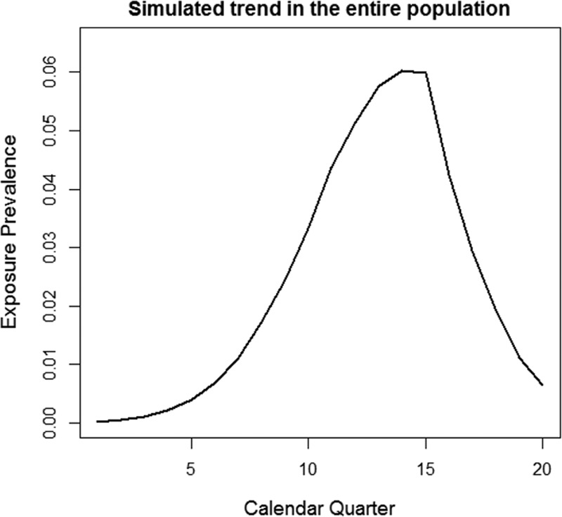
Trend of simulated exposure over 20 calendar quarters. The exposure prevalence goes from 0% in the first quarter to 5% in the 15th quarter and then goes down to almost 0% in the 20th quarter.
Based on the cumulative probabilities of exposure estimated via logistic regression, the study population was stratified into quintiles, that is, K = 5. As expected, these strata, each with 50,000 individuals, had different trends in exposure prevalence. The cumulative probability of exposure model included all five covariates, as shown in Figure 2.
FIGURE 2.
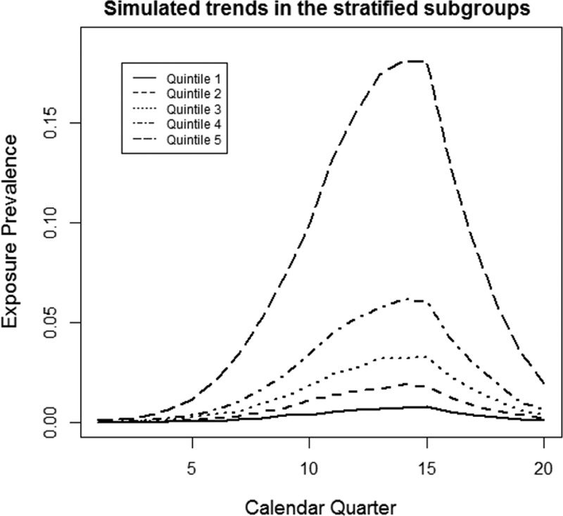
Simulated trends in exposure prevalence for the stratified subgroups based on cumulative probability of exposure quintiles. Each quintile of cumulative probability of exposure exhibits a different trend of exposure prevalence over time. The top quintile has the most dramatic change from base level to peak while the bottom quintile barely changes.
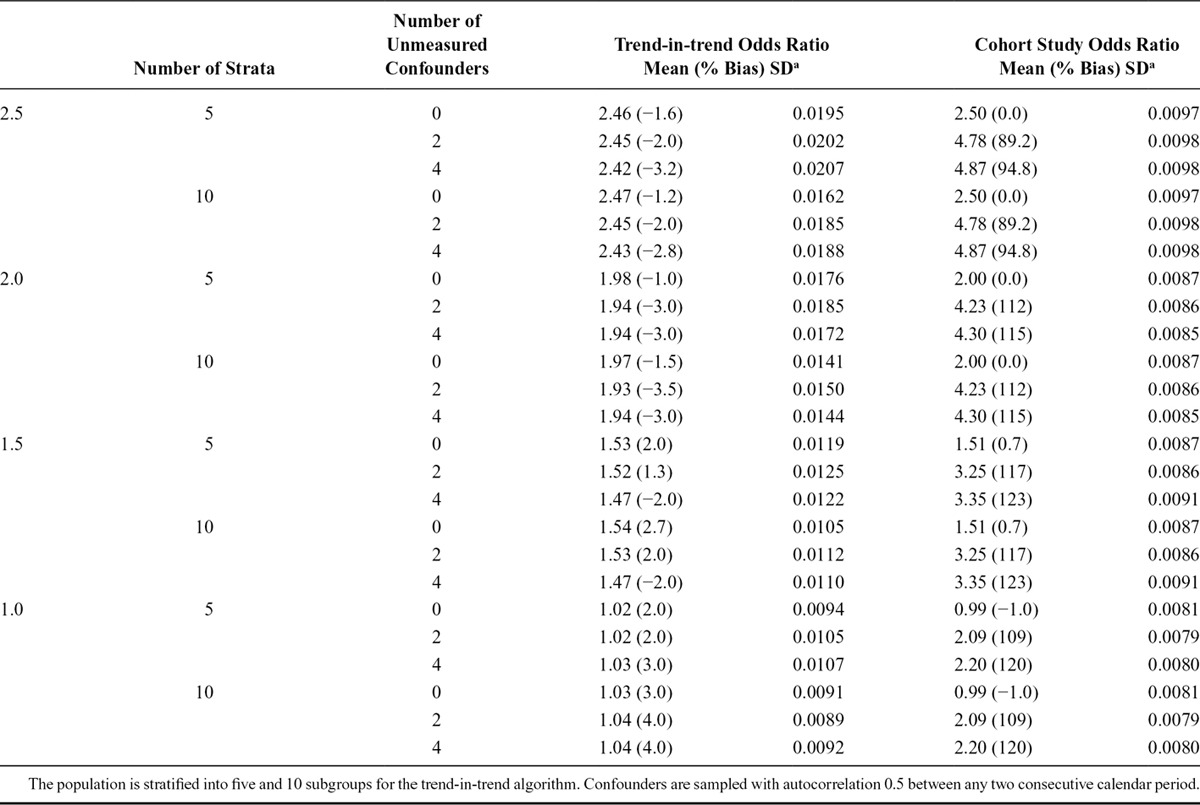
We considered the following scenarios under the rare events assumption: (1) the OR takes values of 1.0, 1.5, 2.0, and 2.5; (2) the strength of the cumulative probability of exposure model has three levels quantified by zero, two, and four omitted confounders out of five confounders in total, and a c statistic is calculated for each level to gauge unobserved heterogeneity in factors affecting outcome; (3) the number of cumulative probability of exposure strata is either five or 10. We compare the estimated OR with those calculated using the cohort method. The results, which are the average values of 1,000 simulations, are summarized in Tables 1–3, corresponding to three different scenarios of covariates sampling as described above.
TABLE 1.
Comparison of the Estimated Causal Odds Ratio Using the Trend-in-trend Design and the Cohort Study Method
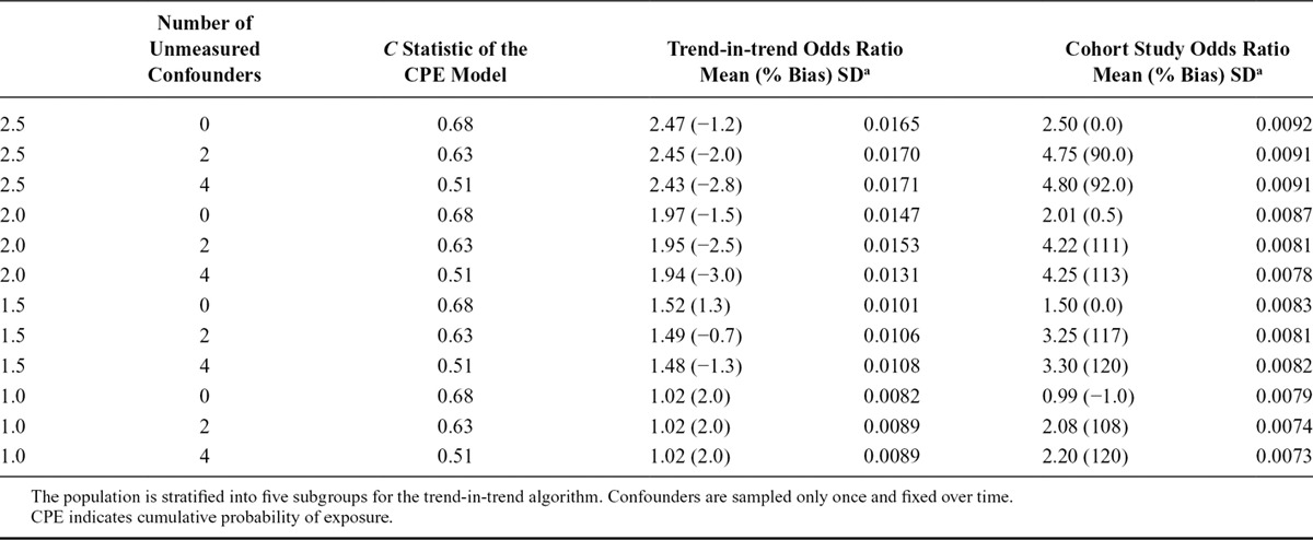
TABLE 3.
Comparison of the Estimated Causal Odds Ratio Using the Trend-in-trend Design and the Cohort Study Method
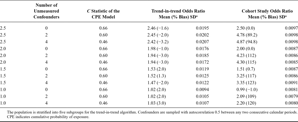
TABLE 2.
Comparison of the Estimated Causal Odds Ratio Using the Trend-in-trend Design and the Cohort Study Method
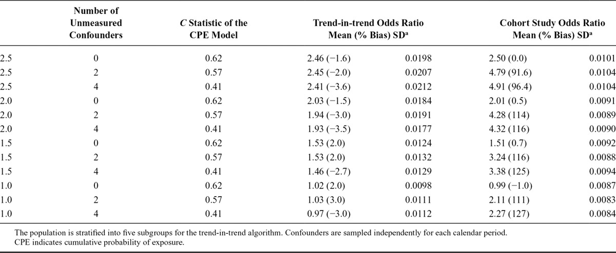
As expected, when there were no unmeasured confounders, both the trend-in-trend and cohort designs yielded ORs that were close to the truth. However, as the number of unmeasured confounders increased, the ORs produced by the cohort design became very biased, with biases ranging from 90% to 127%, while those from the trend-in-trend design remained close to the truth, with bias ranging from −3.5% to 3%. The SDs for the trend-in-trend method were one to two times as large as those for the cohort method, which is to be expected as individual-level information is partially lost when counts of outcomes are aggregated. Furthermore, we observed a reduction in SD for the trend-in-trend method when the number of strata increases from five to 10, as shown in Table 4.
TABLE 4.
Comparison of the Estimated Causal Odds Ratio Using the Trend-in-trend Design and the Cohort Study Method
APPLICATION
We applied the trend-in-trend method to Clinformatics Data Mart Database (OptumInsight, Eden Prairie, MN) to examine association between rofecoxib and AMI, severe hypoglycemia, and nonvertebral bone fracture. The University of Pennsylvania’s Institutional Review Board determined that this study met the eligibility criteria for IRB reviews exemption authorized by 45 CFR 46.101, category 4. Definitions of these outcomes are described in the supplementary materials (http://links.lww.com/EDE/B123). We first identified all persons age 18 years or older in Optum who received one or more prescriptions for rofecoxib during the study period from April 1, 2000 to December 30, 2004. For each rofecoxib-exposed person episode, we ascertained the first month and the last month of their continuous enrollment episode (or episodes, for persons with multiple enrollment episodes) during the study period. Thus, the unit of observation was the enrollment episode, defined as a period of continuous enrollment for a person. A person could contribute multiple episodes. For each rofecoxib-exposed episode, we randomly sampled, without replacement, nine rofecoxib-unexposed enrollment episodes with an enrollment start date on or before no more than 1 year of the rofecoxib-exposed subject’s enrollment start date, and with an enrollment end date on or after the rofecoxib-exposed subject’s enrollment end date. The rationale for this criterion was to ensure sufficient overlap in follow-up calendar time for exposed and unexposed subjects. Thus, the analysis set contained 10 times as many total episodes as there were rofecoxib-exposed enrollment episodes. This was done to improve computational efficiency versus including the entire study population.
We then fit a logistic regression to estimate the cumulative probability of exposure using age, sex, diagnosis of rheumatoid arthritis, and diagnosis of osteoarthritis as explanatory variables. Diagnosis codes for these variables are listed in the supplementary materials (http://links.lww.com/EDE/B123). For rofecoxib-exposed subjects, these covariates were measured at their first prescription date. For control subjects, these covariates were measured the same date as their corresponding exposed subjects. The c statistic was 0.61, which produced good separation of exposure prevalence across quintiles, as shown in Figure 3. The estimated coefficients and SDs (as shown in parentheses) are 0.0228 (0.0001) for continuous age, 0.1458 (0.0027) for female sex, 2.4418 (0.0124) for rheumatoid arthritis, and −0.6444 (0.0191) for osteoarthritis.
FIGURE 3.
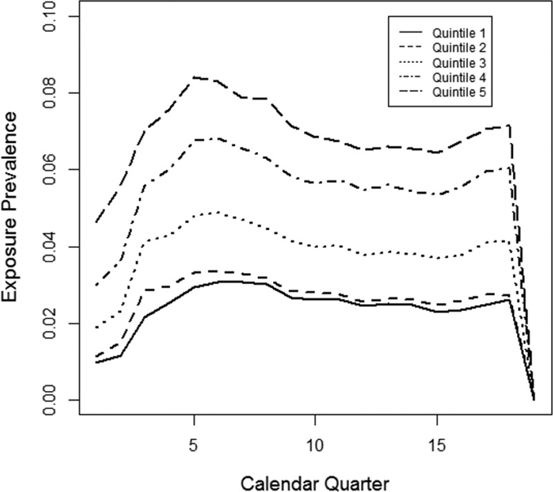
Trends in rofecoxib exposure for the stratified groups using the Optum Clinformatics Database.
The trend-in-trend method yielded an OR (95% confidence interval) for rofecoxib and AMI of 1.2 (1.1, 1.4), which is consistent with the results of prior epidemiologic studies: a 2005 meta-analysis yielded a pooled relative risk of 1.2 (1.1, 1.3) for cohort and nested case–control studies,12 and a more recent meta-analysis reported a pooled relative risk of 1.3 (1.2, 1.5).13 The ORs for the negative control outcomes, severe hypoglycemia and nonvertebral bone fracture (neither of which is thought to be affected by rofecoxib), were 1.1 (0.92, 1.3) and 0.84 (0.64, 1.1), which are both consistent with no effect.14
DISCUSSION
We describe a novel hybrid ecologic-epidemiologic study design called the trend-in-trend design, provide a mathematical derivation of the resulting odds ratio, use simulation to confirm that the results are less biased (albeit somewhat less precise) than those of a cohort study when there is unmeasured confounding, and apply that method to reproduce one positive and two null associations using real-world data. The results of the empiric study using real-world data show that the design is readily applicable and produces expected results.
Importantly, the trend-in-trend design avoids the Achilles’ heel of most epidemiologic studies of healthcare interventions: conflation of receiving a treatment with needing that treatment. Unlike cohort studies, the trend-in-trend design does not assume no unmeasured confounders, but instead examines changes in outcome occurrence as a function of changes in exposure prevalence across strata with differential time trends in exposure. Therefore, the results of a trend-in-trend study will be unconfounded unless there are unmeasured factors affecting outcome for which there are time trends in prevalence that are correlated with time trends in exposure across the strata defined by exposure trend. This could occur if there are co-interventions for which the trend in use is positively correlated with trends in use of the exposure, or alternatives for which the trend in use is negatively correlated with trends in use of the exposure. As the scenarios that would produce a confounded trend-in-trend estimate are a subset of those that would produce a confounded cohort estimate, the trend-in-trend design is more resistant to confounding. However, the trend-in-trend design is feasible only if there is a strong time trend in exposure prevalence. Similarly, the effect estimates produced using calendar period as an IV will be biased if there is any time trend in an unmeasured causal factor, whereas a trend-in-trend study will be biased only if changes in the prevalence of such a factor are correlated with changes in exposure prevalence across cumulative probability of exposure strata. The trend-in-trend design therefore relaxes the assumptions under which use of calendar time as an IV is valid.
The causal contrast examined by the trend-in-trend approach deserves discussion. It is the instantaneous effect of use of the exposure of interest rather than the exposure(s) (if any) that the increasing (or declining) trend in use of the exposure of interest displaced (or was displaced by). In the example of rofecoxib, this is likely to be some combination of nonselective nonsteroidal anti-inflammatory drugs, opioids, and no treatment. Thus, the trend-in-trend results may not mimic the results of placebo-controlled trials evaluating the study treatment. Nevertheless, the causal contrast with the alternatives that it displaces or is displaced by is arguably more relevant from a public health perspective.
The main limitations of the trend-in-trend method are the need for a strong trend in exposure prevalence and the reduced statistical precision that accompanies group-level rather than individual-level analyses. Limitations of the current study include the modest range of scenarios simulated and the fact that there is no empirical example with a causal effect known with complete certainty.
Additional work is needed to improve the utility of the trend-in-trend design. Such work should address control for measured factors for which there may be time trends that are correlated with time trends in exposure across cumulative probability of exposure strata, examination of treatment effect heterogeneity, sequential analysis methods to allow multiple looks while limiting type-1 error, and estimation of statistical power and detectable alternative.
Supplementary Material
Footnotes
Editor’s Note: A commentary on this article appears on p. 537.
This research was supported in part by Grants R01AG025152, R01DK102694, R01HD074756, R01AG040105, and UL1TR000003 from the National Institutes of Health. Data from the simulations reported in this article are provided as supplemental data files; http://links.lww.com/EDE/B123. Because of the agreement governing the University of Pennsylvania’s access to the Optum Clinformatics data, the investigators cannot provide access to these data. Drs. Hennessy and Leonard receive funding through their institution from the US Food and Drug Administration for their roles in the Mini-Sentinel program.
Dr. Hennessy has performed consulting for Merck Sharp & Dohme Corp that is unrelated to rofecoxib. None of the other authors has potential conflict of interest.
Supplemental digital content is available through direct URL citations in the HTML and PDF versions of this article (www.epidem.com).
REFERENCES
- 1.Cook TD, Campbell DT, Day A. Quasi-experimentation: Design & Analysis Issues for Field Settings. 1979Vol. 351 Boston, MA: Houghton Mifflin. [Google Scholar]
- 2.Meirik O. Cohort and case-control studies. 2008Geneva: World Health Organization;. [Google Scholar]
- 3.Viera AJ. Odds ratios and risk ratios: what’s the difference and why does it matter? South Med J. 2008;101:730–734.. [DOI] [PubMed] [Google Scholar]
- 4.Lechner M. The estimation of causal effects by difference-in-difference methods. Now, 2011. [Google Scholar]
- 5.Cain LE, Cole SR, Greenland S, et al. Effect of highly active antiretroviral therapy on incident AIDS using calendar period as an instrumental variable. Am J Epidemiol. 2009:kwp002. [DOI] [PMC free article] [PubMed] [Google Scholar]
- 6.Johnston KM, Gustafson P, Levy AR, Grootendorst P. Use of instrumental variables in the analysis of generalized linear models in the presence of unmeasured confounding with applications to epidemiological research. Stat Med. 2008;27:1539–1556.. [DOI] [PubMed] [Google Scholar]
- 7.Jüni P, Nartey L, Reichenbach S, Sterchi R, Dieppe PA, Egger M. Risk of cardiovascular events and rofecoxib: cumulative meta-analysis. Lancet. 2004;364:2021–2029.. [DOI] [PubMed] [Google Scholar]
- 8.Vestergaard P, Rejnmark L, Mosekilde L. Fracture risk associated with use of nonsteroidal anti-inflammatory drugs, acetylsalicylic acid, and acetaminophen and the effects of rheumatoid arthritis and osteoarthritis. Calcif Tissue Int. 2006;79:84–94.. [DOI] [PubMed] [Google Scholar]
- 9.Rosenbaum PR, Rubin DB. The central role of the propensity score in observational studies for causal effects. Biometrika 1983; 70:41–55.. [Google Scholar]
- 10.Zeger SL, Liang KY, Albert PS. Models for longitudinal data: a generalized estimating equation approach. Biometrics. 1988;44:1049–1060.. [PubMed] [Google Scholar]
- 11.Benjamin EJ, Levy D, Vaziri SM, D’Agostino RB, Belanger AJ, Wolf PA. Independent risk factors for atrial fibrillation in a population-based cohort. The Framingham Heart Study. JAMA. 1994;271:840–844.. [PubMed] [Google Scholar]
- 12.Hernández-Díaz S, Varas-Lorenzo C, García Rodríguez LA. Non-steroidal antiinflammatory drugs and the risk of acute myocardial infarction. Basic Clin Pharmacol Toxicol. 2006;98:266–274.. [DOI] [PubMed] [Google Scholar]
- 13.Varas-Lorenzo C, Riera-Guardia N, Calingaert B, F, et al. Myocardial infarction and individual nonsteroidal anti-inflammatory drugs meta-analysis of observational studies. Pharmacoepidemiol Drug Saf 2013; 22.6:559–570.. [DOI] [PMC free article] [PubMed] [Google Scholar]
- 14.Solomon DH, Rassen JA, Glynn RJ, Lee J, Levin R, Schneeweiss S. The comparative safety of analgesics in older adults with arthritis. Arch Intern Med. 2010;170:1968–1976.. [DOI] [PubMed] [Google Scholar]
- 15.Lévesque LE, Brophy JM, Zhang B. The risk for myocardial infarction with cyclooxygenase-2 inhibitors: a population study of elderly adults. Ann Intern Med. 2005;142:481–489.. [DOI] [PubMed] [Google Scholar]
- 16.Kiyota Y, Schneeweiss S, Glynn RJ, Cannuscio CC, Avorn J, Solomon DH. Accuracy of Medicare claims-based diagnosis of acute myocardial infarction: estimating positive predictive value on the basis of review of hospital records. Am Heart J. 2004;148:99–104.. [DOI] [PubMed] [Google Scholar]
- 17.Ginde AA, Blanc PG, Lieberman RM, Camargo CA., Jr Validation of ICD-9-CM coding algorithm for improved identification of hypoglycemia visits. BMC Endocr Disord. 2008;8: 4. [DOI] [PMC free article] [PubMed] [Google Scholar]
- 18.Heagerty PJ, Zeger SL. Marginalized multilevel models and likelihood inference (with comments and a rejoinder by the authors). Stat Sci. 2000;15:1–26.. [Google Scholar]


